Article

Mapping Winter Wheat Planting Area and Monitoring Its Phenology Using Sentinel-1 Backscatter Time Series

College of Resources and Environmental Sciences, China Agricultural University, Beijing 100193, China
*
Author to whom correspondence should be addressed.
Remote Sens. 2019, 11(4), 449; https://doi.org/10.3390/rs11040449
Submission received: 6 January 2019 / Revised: 15 February 2019 / Accepted: 16 February 2019 / Published: 21 February 2019
(This article belongs to the Special Issue Time Series Analysis Based on SAR Images)

Abstract

:
Crop planting area mapping and phenology monitoring are of great importance to analyzing the impacts of climate change on agricultural production. In this study, crop planting area and phenology were identified based on Sentinel-1 backscatter time series in the test region of the North China Plain, East Asia, which has a stable cropping pattern and similar phenological stages across the region. Ground phenological observations acquired from a typical agro-meteorological station were used as a priori knowledge. A parallelepiped classifier processed VH (vertical transmitting, horizontal receiving) and VV (vertical transmitting, vertical receiving) backscatter signals in order to map the winter wheat planting area. An accuracy assessment showed that the total classification accuracy reached 84% and the Kappa coefficient was 0.77. Both the difference ( σ d ) between VH and VV and its slope were obtained to contrast with a priori knowledge and then used to extract the phenological metrics. Our findings from the analysis of the time series showed that the seedling, tillering, overwintering, jointing, and heading of winter wheat may be closely related to σ d and its slope. Overall, this study presents a generalizable methodology for mapping the winter wheat planting area and monitoring phenology using Sentinel-1 backscatter time series, especially in areas lacking optical remote sensing data. Our results suggest that the main change in Sentinel-1 backscatter is dominated by the vegetation canopy structure, which is different from the established methods using optical remote sensing data, and it is available for phenological metrics extraction.

1. Introduction

Phenology is strongly related to the seasonal dynamics of a growth environment and therefore plays an important role in vegetation monitoring [1,2]. Phenology also controls many types of biophysical and biochemical feedback from vegetation to the climate system [3]. Against the background of global warming, the phenology of many plants has changed, and these shifts are related to climate change [4,5]. For crops, phenology controls the partition of biomass to different organs and is related to the optimal timing of agronomic management options [6,7]. Therefore, understanding the change in phenological phases is helpful for improving agricultural management for higher crop yields and better food quality [8,9].
Field and satellite-based observations are two popular ways of obtaining crop phenological data and information. Usually, measuring and observing crops on farmland directly records phenological information. The development of digital camera technology, the ecosystem phenology camera, and a new method for near-surface remote sensing, has shown great potential for monitoring phenological events [10]. However, the sparsely distributed observational stations with or without digital cameras have limited the representation of large-scale phenology. In contrast, satellite-based observation can offer a practical way to acquire crop information over a large area. With excellent spatial coverage and short revisit times, optical remote sensing data sources such as the Advanced Very-High-Resolution Radiometer (AVHRR), Medium-Resolution Imaging Spectrometer Instrument (MERIS), and Moderate-Resolution Imaging Spectroradiometer (MODIS) have been widely used for regional-scale to global-scale vegetation trend analysis [11,12,13]. Meng et al. [14] developed a method for detecting the key phenological stages of winter wheat in the North China Plain from MERIS time series. Chu et al. [15] used MODIS time series to extract the greening up and heading of winter wheat in the Yellow River Delta from 2012 to 2013. Although these studies have suggested that optical remote sensing would be adequate for phenology extraction over large areas, atmospheric effects such as cloud and haze contamination will always exist and probably lead to large uncertainty in vegetation information.
To overcome these difficulties, it is important to consider the usage of Synthetic Aperture Radar (SAR) [16,17]. Satellite-based imaging radar such as SAR is not limited by cloud cover and has regular revisiting intervals. Sentinel-1 launched in 2014 and 2016, carrying C-band SAR sensors, and is well suited to capturing agricultural land use dynamics for crop mapping [18]. Sentinel-1, as a new SAR data source with better spatiotemporal resolution, has been used for crop monitoring and mapping [19,20,21,22]. For example, Navarro et al. [23] assessed the complementarity of optical and SAR data for crop type classification (maize, soybean, bean, and pasture) and estimated the length of each phenological stage in Angola. Muro et al. [24] used the S1-omnibus, which is a detection approach for Sentinel-1 time series changes, to capture the spatiotemporal changes produced by water surface dynamics in wetlands and agricultural practices in farmlands. In addition, SAR time series were also used to monitor the phenology of rice and winter rapeseed [25,26]. However, there are no studies that have investigated winter wheat phenology using Sentinel-1 backscatter time series even though wheat feeds about 40% of the world’s population and occupies a central position in maintaining the world’s food security [27]. Vreugdenhil et al. proposed that Sentinel-1 backscatter time series have potential for monitoring crop phenology [28]. Based on their findings, our study tried to generalize a methodology using SAR time series to monitor winter wheat.
This study aims to assess the potential of Sentinel-1 satellite SAR imagery for mapping a winter wheat planting area and further monitoring phenology when optimal remote sensing data are not available due to atmospheric effects such as cloud and haze contamination. For this purpose, we focused on a test region in the North China Plain, which is a staple wheat-producing area of China. The SAR data were used for mapping winter wheat planting area based on a method using a parallelepiped classifier and reconstructing the backscatter time series. Furthermore, phenological metrics were extracted from dual-polarization (VV, VH) backscattering time series based on a priori knowledge. Lastly, our study will help (1) distinguish the winter wheat planting area from other land types, (2) explain how the backscatter signatures change during the winter wheat growing season, and (3) monitor winter wheat phenology using a stable and robust data source.

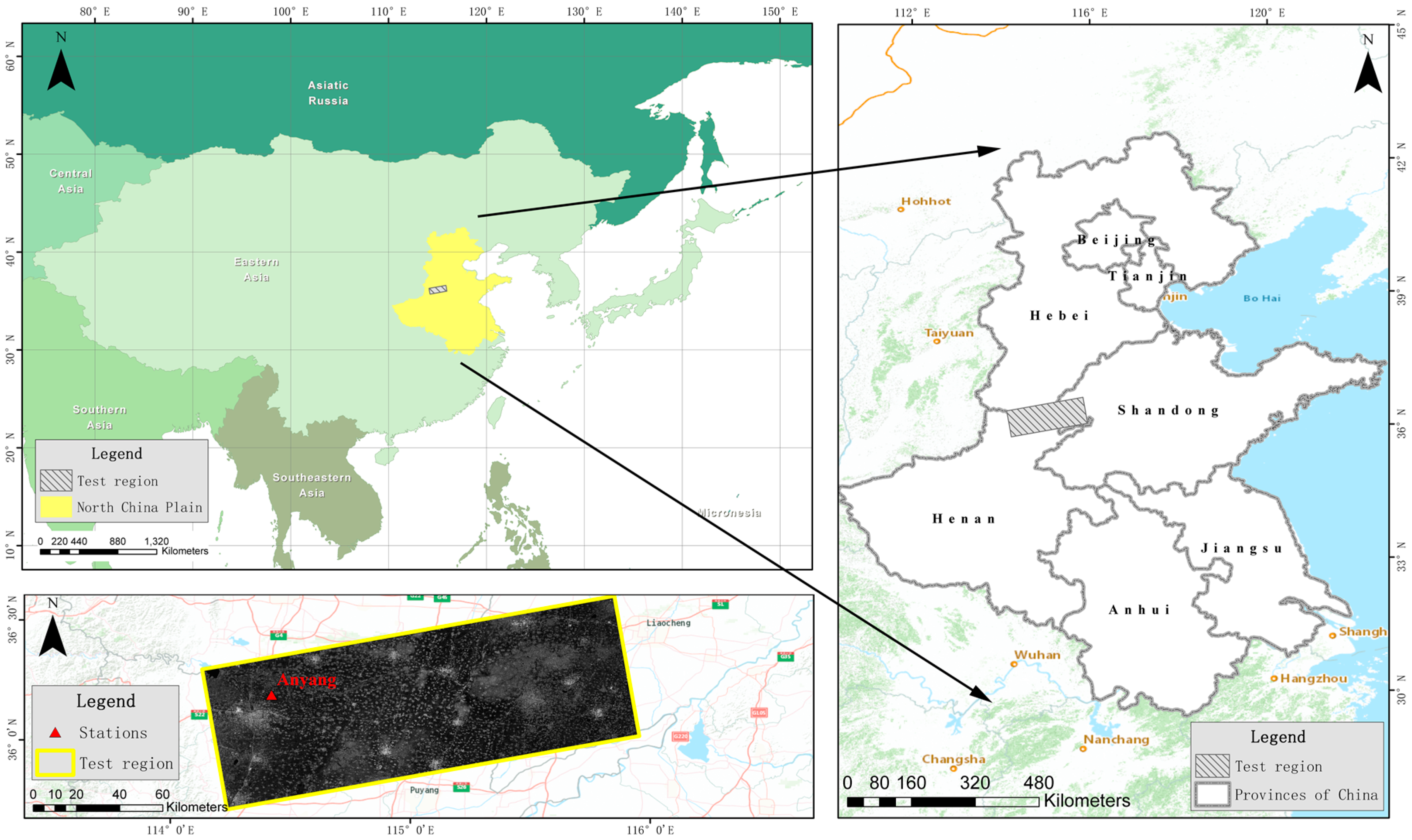
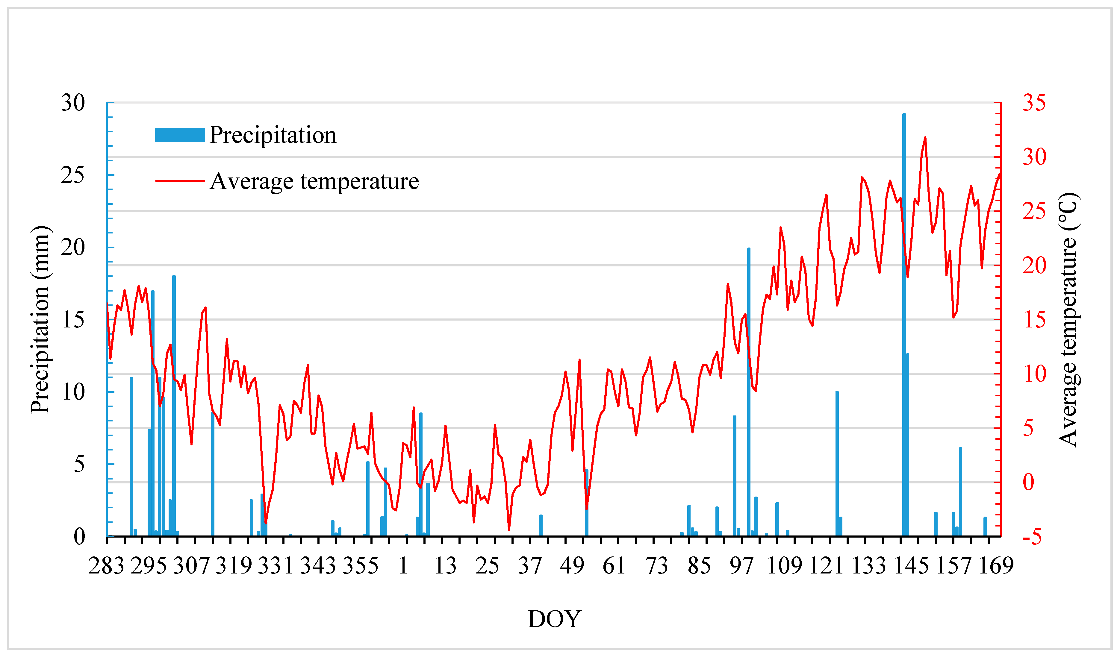
2. Study Area and Data

The test region considered in this study is located in the central part of the North China Plain (NCP) at the juncture of the Hebei, Shandong, and Henan provinces of China (Figure 1). The North China Plain is the second largest plain in China, including Beijing and Tianjin as well as the Hebei, Shandong, Henan, Anhui, and Jiangsu provinces. In the NCP, winter wheat is the main food crop, which occupied about 20% of the entire crop output of China, and therefore plays a vital role in guaranteeing grain security in East Asia [29,30]. Generally, winter wheat is sowed in early October of every year and harvested in early to the middle of June of the following year (Table 1).
Sentinel-1 can operate in four modes—Interferometric Wide Swath (IW), Extra Wide Swath (EW), Wave (WV), and Stripmap (SM)—with different resolutions, extents, incidence angles, and polarizations. In this study, we used Sentinel-1A C-band IW mode Ground Range Detected High-Resolution (GRDH) images, which were requested from ESA (European Space Agency), with high spatial (10 m) and stable temporal (12 days now and 6 days in the future) resolution. The IW mode GRDH, as the pre-defined mode over land, provides dual-polarization imagery: VV (vertical transmitting, vertical receiving) and VH (vertical transmitting, horizontal receiving). Twenty-two Sentinel-1A images, acquired between 9 October 2016 and 30 June 2017 (Table 2), cover the entire test region with a revisit time of 12 days.
The meteorological data and grou nd phenological observations of the test region were archived at the National Meteorological Information Center (NMIC) of China. During the growing season, the precipitation mainly happened in October 2016 and May 2017 (Figure 2). The precipitation affects the SAR backscatter significantly, especially in the early growth stage of winter wheat with bare soil. In addition, more precipitation during the growing season means a large amount of cloudy days in this area which lead to unavailable optical remote sensing data. In addition, phenological observations at an agro-meteorological experimental station (Anyang station) were used as a priori knowledge (Figure 1). The beginning dates of the 11 wheat growth stages were recorded at the agro-meteorological experimental station (Table 3).

3. Methodology

3.1. SAR Data Pre-Processing

Sentinel-1A data were pre-processed using ESA’s open source Sentinel-1 Toolbox, SNAP. The pre-processing steps mainly included the orbit correction, radiometric calibration, and Range-Doppler terrain correction. The data were first calibrated to obtain the sigma0 backscatter coefficient, and then applied to accurately geocode the images using a digital elevation model. Batch Processing and Graph Builder in SNAP were used to batch all these pre-processing steps and convert the linear values to dB values. All the SAR images were converted from power scale values into logarithmic scale values to correctly represent dB values using the following equation:
σ i ( d B ) = 10 × log 10 ( σ i )
where σ i is the sigma-calibrated backscattering coefficient obtained from SNAP pre-processing for each pixel of the SAR images [23]. Meanwhile, the regions of interest (ROIs) were selected as the affirmed winter wheat planting area based on experiential knowledge and fieldwork.

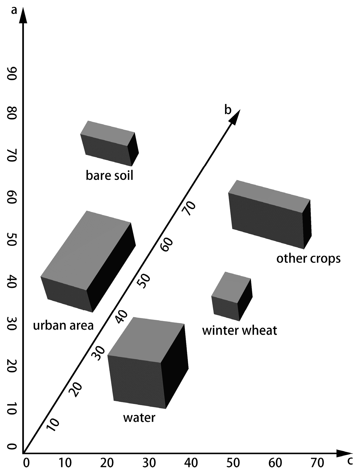
3.2. Classification Method

A parallelepiped classifier, which is a supervised classification method, was used to classify the images of the test region to map the winter wheat planting area. The method is based on the division of every axis of a multidimensional feature vector, and it is one of the most simple and accurate classification techniques [31]. For each class, the lowest and highest values on each axis are used to define the decision boundary (Figure 3) [32,33]. The parallelepiped classifier allows multidimensional boxes that are used for multispectral bands [34]. Therefore, all the images we acquired—22 VV images and 22 VH images—were stacked into one image with 44 bands. The 44 bands as 44-dimensional feature vectors were used to classify and map the winter wheat planting area in the test region, i.e., every axis was the backscatter signatures of one VV or VH image on a certain date during the growing season. In this study, a parallelepiped classifier was used to classify and extract the winter wheat planting area from among other classes (urban area, other crops, water, and bare soil).

3.3. Time Series Reconstruction

After pre-processing, we reconstructed time series from Sentinel-1A images to analyze the backscatter signatures tied to winter wheat phenology. The backscatter signatures of Sentinel-1A in different phenological stages represent information on the canopy structure and physiological traits of crops which is related to the vegetation coverage and field management [25]. Different backscatter signatures could be found even in one winter wheat field due to speckle and other noise-like influences. Therefore, filtering the backscatter time series was necessary and had the purpose of reducing the short-term influence of environmental conditions.
A filter algorithm called HANTS (Harmonic Analysis of Time Series) is used to smooth noisy data and can be an appropriate tool to describe the temporal behavior of remote sensing parameters [35]. This algorithm is implemented by calculating a Fourier series for the data while the Fourier transform determines the values of the filtering outliers. It is one of the fastest filter methods for smoothing and reconstructing time series of remote sensing parameters [36]. An easily operated tool known as the IDL (Interactive Data Language) version of HANTS was used in this study. Hence, the smoothed backscatter signals were used for analyzing the winter wheat backscatter time series and extracting the phenological metrics.

3.4. Phenological Metrics Extraction

Using an equation to combine both VV and VH images could reduce the ground and vegetation interaction effects (e.g., double-bounce) and eliminate the errors of the acquisition system or environmental factors. In previous studies, a cross ratio between VH and VV was calculated as VH/VV in the linear domain and then converted to the logarithmic domain [28,37]. Therefore, in this study, VH and VV were converted to the logarithmic domain first in pre-processing according to Equation (1). Then, the difference between VH and VV was calculated according to the following equation:
σ d ( d B ) = σ v h σ v v
where σ d is the difference between VH and VV, and σ v v and σ v h are the dB values of the VV and VH images, respectively.
Although some previous studies also utilized the cross ratio VH/VV to understand the temporal behavior of crops, the smoothed backscatter time series in this study was used to derive the winter wheat phenology metrics. Based on a priori knowledge obtained from ground phenological observations, a one-on-one correspondence relationship between the phenological stages and the specific points of the time series was created. In addition, we also analyzed the slope of the σ d (VH-VV) time series to find some other specific points. Lastly, the specific points in both σ d and its slope curve were inferred as phenological metrics and then used to monitor the winter wheat phenology.

4. Results and Discussion

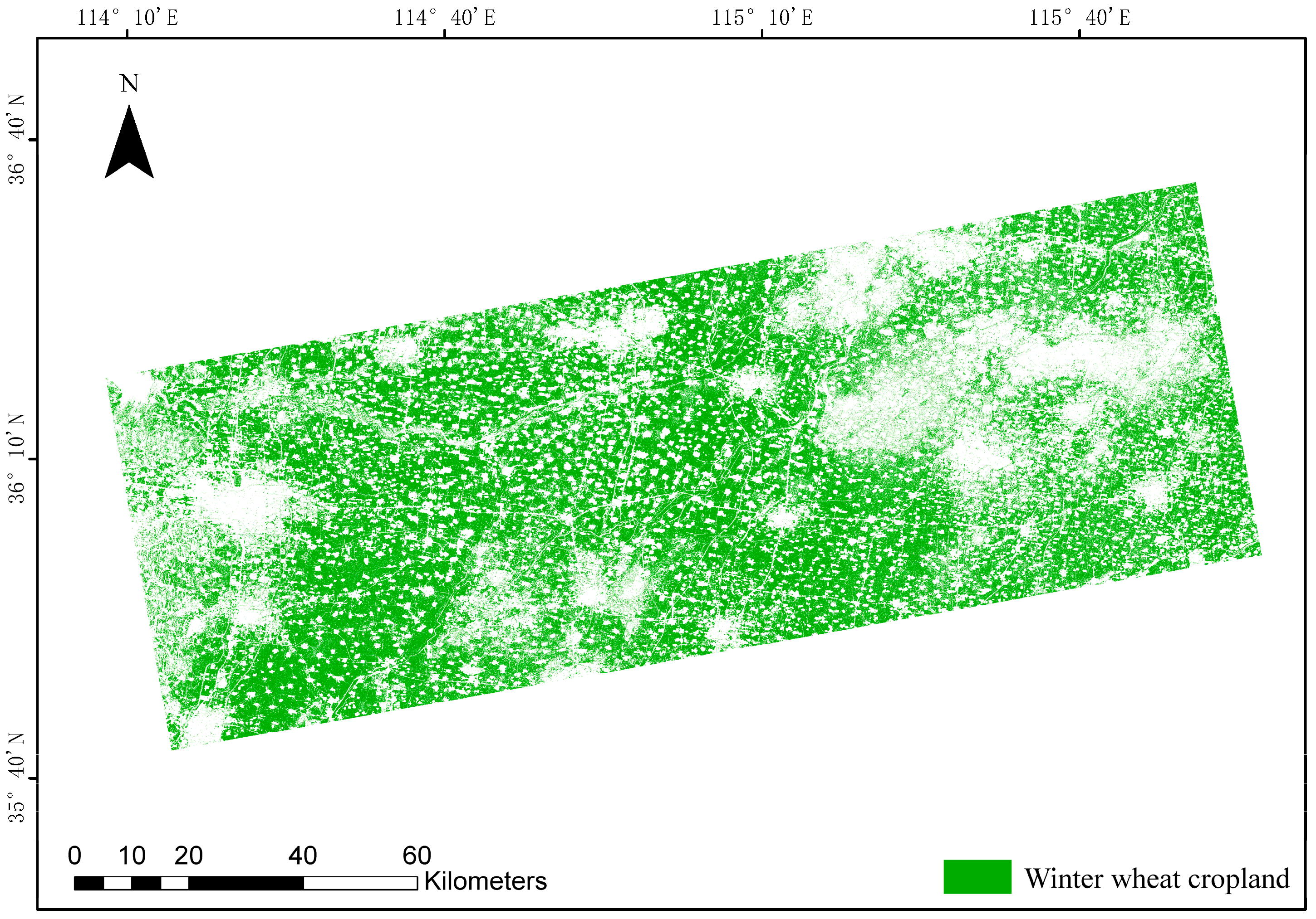
4.1. Mapping the Sentinel-1-Derived Winter Wheat Planting Area

Figure 4 shows the temporal backscatter coefficient profiles of land cover types selected from ROIs at both VV and VH polarization from 9 October 2016 to 30 June 2017. The results show that the mean σ v v values of winter wheat, urban, other crops, water, and bare soil during the winter wheat growth period were −14.46, −7.08, −11.26, −19.70, and −9.76 dB, respectively. The mean σ v h values were −20.68, −13.65, −18.54, −23.94, and −16.65 dB, respectively. In addition, although most of the temporal backscatter profiles in σ v v were relatively independent and separable, the backscatter coefficients at VH polarization provided an alternative at a different polarization mode. Overall, the results indicate that it is feasible to distinguish winter wheat from other land cover types and map the winter wheat planting area using Sentinel-1.
Figure 5 illustrates a map of the winter wheat planting area from the multi-temporal stacked dual-polarization bands based on the parallelepiped classifier. Analyzing the results of the confusion matrix, the total accuracy of our classification was 84% and the Kappa coefficient was 0.77. Previous research has shown that many more classification methods could improve the accuracy of crop mapping [38,39]. However, the method we chose in this case is relatively simple and sufficiently accurate. In addition, it should be noted that this study focused on the representative and pure classification results even though they tended to underestimate the true planting extent.

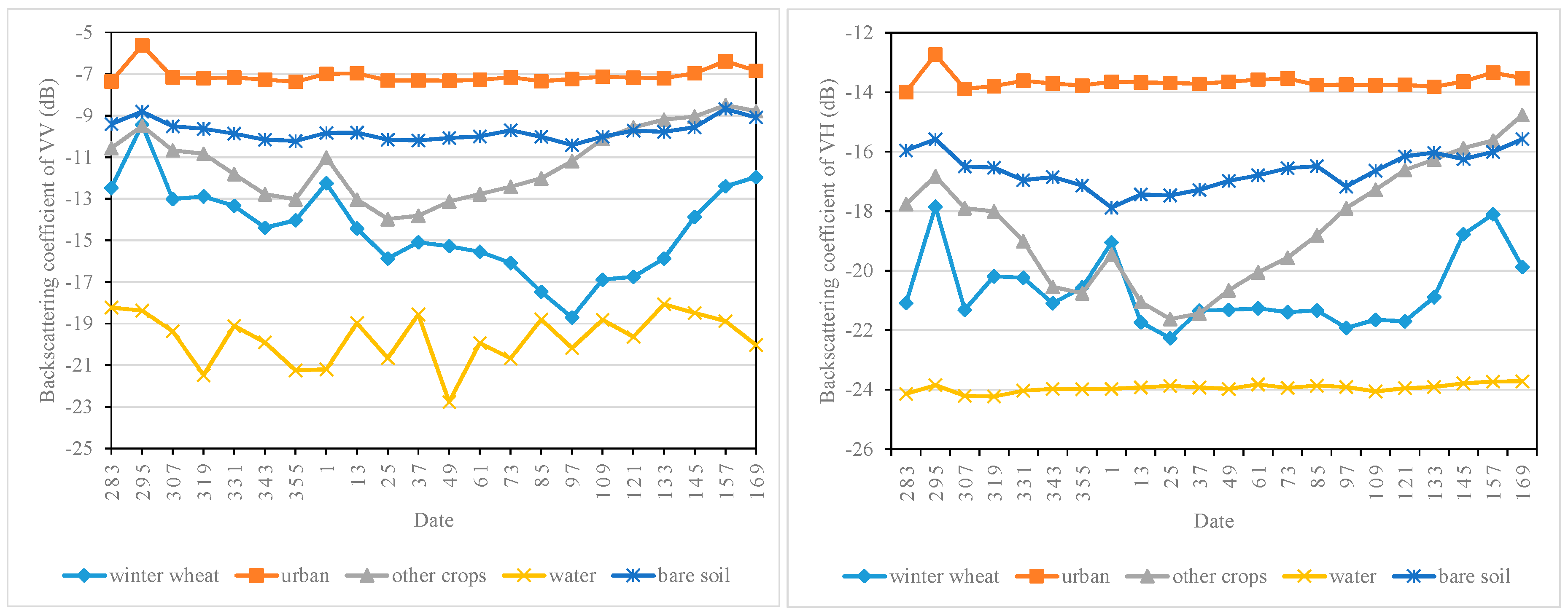
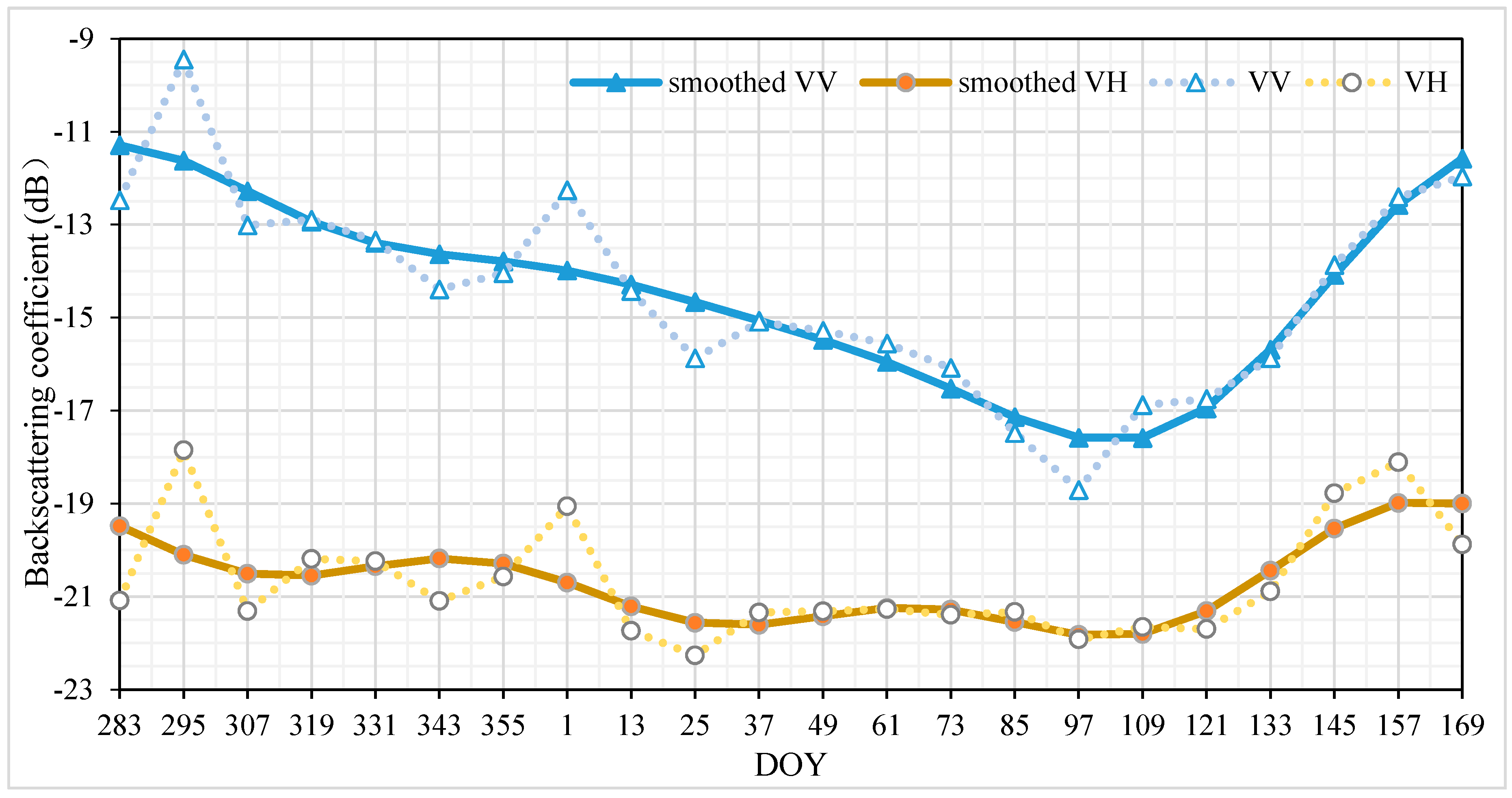
4.2. Analysis of the Winter Wheat Backscatter Time Series

Winter wheat is a kind of narrow-leaf cereal crop that is planted in the autumn, remains in the vegetative phase during the winter, and resumes growth in early spring. In Figure 6, both the smoothed and unsmoothed backscatter time series of the test region show the winter wheat growing season from 9 October 2016 (DOY 283) to 30 June 2017 (DOY 169). Although the results show that the unsmoothed VV and VH profiles were complex and fluctuated, the physical structural properties of the target could explain most of their variations. In addition, the smoothed VV and VH time series based on the HANTS algorithm did not exhibit strong variations but looked relatively smooth, like NDVI (Normalized Difference Vegetation Index) from optical remote sensing [15].
Based on a priori knowledge, winter wheat was planted in early October (around DOY 285) and went into the overwintering stage around DOY 1 in this case. During these stages (sowing, seedling, tillering, and overwintering), the winter wheat began to emerge and developed into young plants above the bare soil of the ground surface. For the unsmoothed backscatter time series, the results show that large variations occurred in VV and VH before the greening up stage of the winter wheat (before DOY 49). Previous research has indicated that VH and VV could contain the interaction between vegetation and the ground caused by stem–ground double scattering [40,41,42]. VV and VH were affected mostly by changes in the soil backscatter driven by soil water content and roughness. This means that rainfall events may explain the increase in the backscatter. At DOY 295 and DOY 1 in particular, there were two peaks of the unsmoothed time series mainly caused by rainfall and frozen soils. Vreugdenhil et al. in Austria also observed this phenomenon for winter cereals [28].
For the smoothed backscatter time series, the results showed that there were differences between the curves of the VV and VH backscatter signals. VV backscatter decreased with the germination and growth of winter wheat and had a small flat curve before the overwintering period (around DOY 1), then kept decreasing steadily until the end of the stem extension phase, and increased rapidly until the harvest season. The minimum of VV occurred around DOY 109, which could be the end of the booting stage and the start of the heading stage. Although it might seem that the change in VV was related to the leaf area index (LAI), the emergence of wheatear and the number of stems should also be considered. Therefore, the canopy structure and the scattering mechanisms of crops mostly likely drove the changes in VV [43,44,45]. Furthermore, the VH backscatter time series appeared to be a wave curve with several peaks and troughs dominated by double-bounce and volume scattering mechanisms [46,47]. Although the VH backscatter signal profile might seem to have no distinct rule, it was likely a result of ground and vegetation interaction. For example, during the tillering stage (around DOY 319 to DOY 1), the increase in VH was most likely caused by an increase in the volume fraction of the vegetation, while the decrease in VH was driven by frozen soils during the overwintering period. In addition, a small increase in VH related to the increase in the number of stems was also found at the greening up stage of the winter wheat (around DOY 49). Hence, the contributions of ground and vegetation interaction (e.g., double-bounce) and volume scattering mechanisms could lead to the changes in the VH backscatter.
The differences in the smoothed backscatter time series in the different growth stages of winter wheat, such as tillering, overwintering, greening up, jointing, booting, and heading provided key information and the possibility for monitoring phenology. The results indicate that the phenological metrics of winter wheat could be extracted by analyzing the backscatter time series. In addition, it should be noted that this study examined only one winter wheat growth cycle and lacks a comparison with different crop calendars.

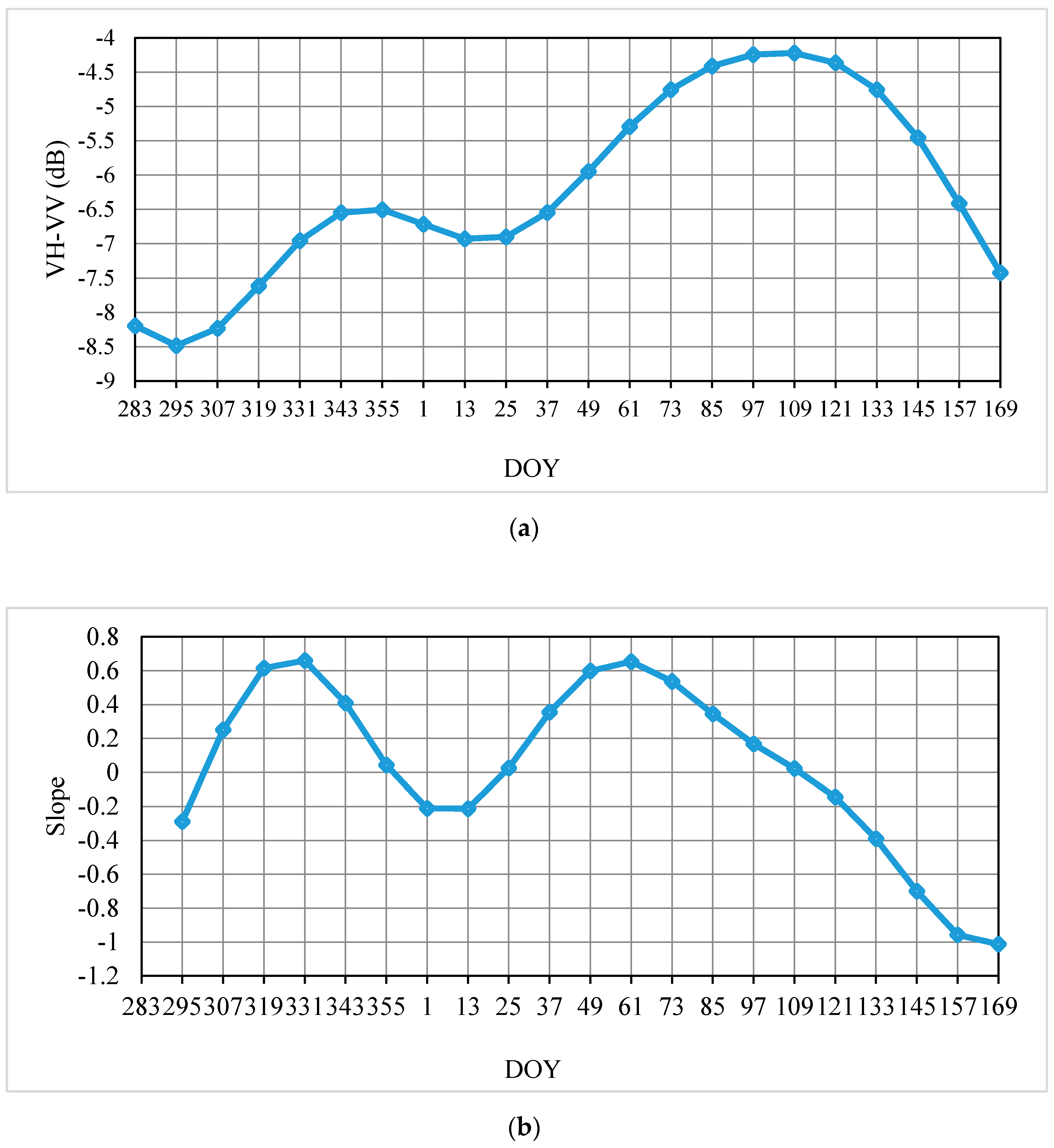
4.3. Monitoring of Winter Wheat Phenology

The time series of σ d (VH-VV) is shown for the growing season of winter wheat from 9 October 2016 (DOY 283) to 30 June 2017 (DOY 169) in Figure 7a. Clearly, a complete time series of σ d consisted of two peaks and two troughs in an entire winter wheat growing season. While the crop started to grow slowly from sowing (around DOY 280), a trough occurred at DOY 295, which was likely driven by a soil roughness change due to rainfall. A steady increase in σ d can be observed from the first trough at DOY 295, which was during the seedling and tillering stage of the winter wheat. The increase in σ d became slow before the winter and then reached the peak visible at DOY 355. This first peak in σ d was likely caused by the tillering of winter wheat. It should be noted that σ d started to decrease at DOY 355 before the overwintering stage (observed at DOY 12). This was likely driven by the slow growth of winter wheat due to the decrease in air temperature. A trough around DOY 13 and DOY 25 was observed during the overwintering stage and was most likely driven by the cold weather which retarded development of the crop and further changed the canopy structure. A steady increase in σ d can be seen from DOY 25, which was the beginning of the greening up stage of the winter wheat. During the jointing and booting stages, the increase continued and reached its maximum at the beginning of the heading stage (around DOY 109), mainly due to the increase in canopy saturation and canopy thickness. Thereafter, σ d started to decrease, which was mostly due to the decline in the leaf area index (LAI) and the change in canopy structure. The decrease was also likely related to the appearance of the wheat spike. Although some previous research suggested that VH/VV, which we called σ d , should be correlated with vegetation water content and fresh biomass, our results indicated that σ d was more strongly correlated with the canopy structure and vegetation coverage [28,36].
The slope of the σ d (VH-VV) time series is also presented in Figure 7b. The results show that there were some other curve characteristics in the slope of the σ d time series which could be considered as additional information for extracting phenological metrics. For example, the first peak (DOY 331) in the slope curve was at the tillering stage, which is one of the periods of fastest growth, and is likely a result of the increase in the number of stems. The maximum value occurred at DOY 61 during the jointing stage and was most likely caused by changes in vertical structure, such as stem extension. In addition, the slope curve is mostly negative from DOY 355 to DOY 25, which means that the overwintering stage faded in and out and lasted longer than expected.
Table 4 lists the main phenological metrics of the Sentinel-1 backscatter time series. The results suggest that some of the growth stages of winter wheat, such as seedling, tillering, overwintering, jointing, and heading, could be identified from σ d and its slope value. Although some other growth stages could not be identified in this case, our study has thrown light on the monitoring of winter wheat using Sentinel-1 backscatter time series. The results indicate that inflection points both in the σ d time series and in the slope curve could be correlated with phenological metrics. Compared with the previous studies using optical remote sensing data, there were fewer atmospheric effects (e.g., cloud, haze) on the C-band SAR data, which would lead to a better and steadier temporal resolution [10,48]. In addition, it should be noted that the phenological metrics based on the analysis of backscatter time series have shown the main changes in the canopy structure (e.g., vertical structure, vegetation coverage) which are different than those in previous research based on NDVI or other vegetation indices [49,50].

5. Conclusions

In this study, we introduced a methodology to map the winter wheat planting area and further monitor phenology using Sentinel-1 SAR data, especially in areas lacking optical remote sensing data due to atmospheric effects such as cloud and haze contamination. This study used a parallelepiped classifier to map the winter wheat planting area. Using this approach, the representative and pure winter wheat planting area was extracted using Sentinel-1 SAR data. By comparing this with ground phenological observations as a priori knowledge, the σ d time series and its slope curve derived from VV and VH backscatter signals were found to be closely related to the seedling, tillering, overwintering, jointing, and heading stages of winter wheat. Time series analysis demonstrated that the VV and VH backscatter signals were correlated with the vegetation canopy structure and vegetation coverage. These findings were achieved without using MODIS or other optical remote sensing data. The presented research also provides valuable insights into ultimately monitoring phenology using backscatter time series via a steady and robust approach. Although some other growth stages could not be identified in this case, it does show the potential for phenological information to be obtained from Sentinel-1 SAR data. Further studies should focus on applying the method developed by our study to a larger region of interest and comparing the crop phenology of different planting regions. We hope more researchers will join us in exploring the application of SAR to agriculture using Sentinel-1 data.

Author Contributions

Y.S. and J.W. conceived and designed the research. Y.S. performed the research, analyzed, and interpreted the data. All authors contributed to the writing of the manuscript.

Funding

The National Key Research and Development Program of China (2016YFD0300105) supported this research.

Acknowledgments

We thank the anonymous reviewers and the editors for their thoughtful comments that helped improve this research. We thank ESA, NMIC, and CAU for providing Sentinel-1 data, the meteorological data, and ground phenological observations. Furthermore, the authors would like to thank Wenke Li, Huiqing Bai, Mingxia Huang, Junqing Zheng, Na Wang, Yang Li, Fuwei He, Xueqing Ma, and other members of our team.

Conflicts of Interest

The authors declare no conflict of interest.

References

  1. Schwartz, M.D. Green-wave phenology. Nature 1998, 394, 839–840. [Google Scholar] [CrossRef]
  2. White, M.A.; Thornton, P.E.; Running, S.W. A continental phenology model for monitoring vegetation responses to interannual climatic variability. Glob. Biogeochem. Cycles 1997, 11, 217–234. [Google Scholar] [CrossRef] [Green Version]
  3. Richardson, A.D.; Keenan, T.F.; Migliavacca, M.; Ryu, Y.; Sonnentag, O.; Toomey, M. Climate change, phenology, and phenological control of vegetation feedbacks to the climate system. Agric. For. Meteorol. 2013, 169, 156–173. [Google Scholar] [CrossRef]
  4. Korner, C.; Basler, D. Phenology Under Global Warming. Science 2010, 327, 1461–1462. [Google Scholar] [CrossRef] [PubMed]
  5. Post, E.; Steinman, B.A.; Mann, M.E. Acceleration of phenological advance and warming with latitude over the past century. Sci. Rep. UK 2018, 8. [Google Scholar] [CrossRef] [PubMed]
  6. Wang, J.; Wang, E.L.; Feng, L.P.; Yin, H.; Yu, W.D. Phenological trends of winter wheat in response to varietal and temperature changes in the North China Plain. Field Crops Res. 2013, 144, 135–144. [Google Scholar] [CrossRef]
  7. Wang, N.; Wang, J.; Wang, E.L.; Yu, Q.; Shi, Y.; He, D. Increased uncertainty in simulated maize phenology with more frequent supra-optimal temperature under climate warming. Eur. J. Agron. 2015, 71, 19–33. [Google Scholar] [CrossRef]
  8. Wielgolaski, F.E. Phenology in agriculture. In Phenology and Seasonality Modeling; Springer: Berlin, Germany, 1974; pp. 369–381. ISBN 3-540-06524-5. [Google Scholar]
  9. Schwartz, M.D. Phenology: An Integrative Environmental Science, 2nd ed.; Springer: Berlin, Germany, 2003; pp. 331–343. ISBN 978-94-007-6924-3. [Google Scholar]
  10. Zhou, L.; He, H.L.; Sun, X.M.; Zhang, L.; Yu, G.R.; Ren, X.L.; Wang, J.Y.; Zhao, F.H. Modeling winter wheat phenology and carbon dioxide fluxes at the ecosystem scale based on digital photography and eddy covariance data. Ecol. Inform. 2013, 18, 69–78. [Google Scholar] [CrossRef]
  11. Tao, J.B.; Wu, W.B.; Zhou, Y.; Wang, Y.; Jiang, Y. Mapping winter wheat using phenological feature of peak before winter on the North China Plain based on time-series MODIS data. J. Integr. Agric. 2017, 16, 348–359. [Google Scholar] [CrossRef]
  12. Liu, J.H.; Zhu, W.Q.; Atzberger, C.; Zhao, A.Z.; Pan, Y.Z.; Huang, X. A Phenology-Based Method to Map Cropping Patterns under a Wheat-Maize Rotation Using Remotely Sensed Time-Series Data. Remote Sens. 2018, 10, 1203. [Google Scholar] [CrossRef]
  13. Kang, W.P.; Wang, T.; Liu, S.L. The Response of Vegetation Phenology and Productivity to Drought in Semi-Arid Regions of Northern China. Remote Sens. 2018, 10, 727. [Google Scholar] [CrossRef]
  14. Meng, J.H.; Wu, B.F.; Li, Q.Z.; Du, X.; Jia, K. Monitoring crop phenology with MERIS data—A case study of winter wheat in North China Plain. In Proceedings of the Electromagnetics Research Symposium, Beijing, China, 23–27 March 2009; pp. 1225–1228. [Google Scholar]
  15. Chu, L.; Huang, C.; Liu, Q.S.; Liu, G.H. Estimation of winter wheat phenology under the influence of cumulative temperature and soil salinity in the Yellow River Delta, China, using MODIS time-series data. Int. J. Remote Sens. 2016, 37, 2211–2232. [Google Scholar] [CrossRef]
  16. Ruetschi, M.; Schaepman, M.E.; Small, D. Using Multitemporal Sentinel-1 C-band Backscatter to Monitor Phenology and Classify Deciduous and Coniferous Forests in Northern Switzerland. Remote Sens. 2018, 10, 55. [Google Scholar] [CrossRef]
  17. Steele-Dunne, S.C.; McNairn, H.; Monsivais-Huertero, A.; Judge, J.; Liu, P.W.; Papathanassiou, K. Radar Remote Sensing of Agricultural Canopies: A Review. IEEE J. Sel. Top. Appl. Earth Obs. Remote Sens. 2017, 10, 2249–2273. [Google Scholar] [CrossRef] [Green Version]
  18. Bargiel, D. A new method for crop classification combining time series of radar images and crop phenology information. Remote Sens. Environ. 2017, 198, 369–383. [Google Scholar] [CrossRef]
  19. Clauss, K.; Ottinger, M.; Leinenkugel, P.; Kuenzer, C. Estimating rice production in the Mekong Delta, Vietnam, utilizing time series of Sentinel-1 SAR data. Int. J. Appl. Earth Obs. 2018, 73, 574–585. [Google Scholar] [CrossRef]
  20. Steinhausen, M.J.; Wagner, P.D.; Narasimhan, B.; Waske, B. Combining Sentinel-1 and Sentinel-2 data for improved land use and land cover mapping of monsoon regions. Int. J. Appl. Earth Obs. 2018, 73, 595–604. [Google Scholar] [CrossRef]
  21. Van Tricht, K.; Gobin, A.; Gilliams, S.; Piccard, I. Synergistic Use of Radar Sentinel-1 and Optical Sentinel-2 Imagery for Crop Mapping: A Case Study for Belgium. Remote Sens. 2018, 10, 1642. [Google Scholar] [CrossRef]
  22. Gao, Q.; Zribi, M.; Escorihuela, M.J.; Baghdadi, N.; Segui, P.Q. Irrigation Mapping Using Sentinel-1 Time Series at Field Scale. Remote Sens. 2018, 10, 1495. [Google Scholar] [CrossRef]
  23. Navarro, A.; Rolim, J.; Miguel, I.; Catalao, J.; Silva, J.; Painho, M.; Vekerdy, Z. Crop Monitoring Based on SPOT-5 Take-5 and Sentinel-1A Data for the Estimation of Crop Water Requirements. Remote Sens. 2016, 8, 525. [Google Scholar] [CrossRef]
  24. Muro, J.; Canty, M.; Conradsen, K.; Huttich, C.; Nielsen, A.A.; Skriver, H.; Remy, F.; Strauch, A.; Thonfeld, F.; Menz, G. Short-Term Change Detection in Wetlands Using Sentinel-1 Time Series. Remote Sens. 2016, 8, 795. [Google Scholar] [CrossRef]
  25. Torbick, N.; Chowdhury, D.; Salas, W.; Qi, J.G. Monitoring Rice Agriculture across Myanmar Using Time Series Sentinel-1 Assisted by Landsat-8 and PALSAR-2. Remote Sens. 2017, 9, 119. [Google Scholar] [CrossRef]
  26. Nguyen, D.B.; Wagner, W. European Rice Cropland Mapping with Sentinel-1 Data: The Mediterranean Region Case Study. Water 2017, 9, 392. [Google Scholar] [CrossRef]
  27. Asif, M.; Iqbal, M.; Randhawa, H.; Spaner, D. Wheat: The miracle cereal. In Managing and Breeding Wheat for Organic Systems; Springer: Berlin, Germany, 2014; pp. 1–7. ISBN 978-3-319-05001-0. [Google Scholar]
  28. Vreugdenhil, M.; Wagner, W.; Bauer-Marschallinger, B.; Pfeil, I.; Teubner, I.; Rudiger, C.; Strauss, P. Sensitivity of Sentinel-1 Backscatter to Vegetation Dynamics: An Austrian Case Study. Remote Sens. 2018, 10, 1396. [Google Scholar] [CrossRef]
  29. Shi, Y.; Li, Y.T.; Xiang, X.J.; Sun, R.B.; Yang, T.; He, D.; Zhang, K.P.; Ni, Y.Y.; Zhu, Y.G.; Adams, J.M.; et al. Spatial scale affects the relative role of stochasticity versus determinism in soil bacterial communities in wheat fields across the North China Plain. Microbiome 2018, 6, 27. [Google Scholar] [CrossRef] [PubMed] [Green Version]
  30. Jeong, S.J.; Ho, C.H.; Piao, S.L.; Kim, J.; Ciais, P.; Lee, Y.B.; Jhun, J.G.; Park, S.K. Effects of double cropping on summer climate of the North China Plain and neighbouring regions. Nat. Clim. Chang. 2014, 4, 615–619. [Google Scholar] [CrossRef] [Green Version]
  31. Castillejo-Gonzalez, I.L.; Lopez-Granados, F.; Garcia-Ferrer, A.; Pena-Barragan, J.M.; Jurado-Exposito, M.; de la Orden, M.S.; Gonzalez-Audicana, M. Object- and pixel-based analysis for mapping crops and their agro-environmental associated measures using QuickBird imagery. Comput. Electron. Agric. 2009, 68, 207–215. [Google Scholar] [CrossRef]
  32. Jog, S.; Dixit, M. Supervised Classification of Satellite Images. In Proceedings of the 2016 Conference on Advances in Signal Processing (CASP), Pune, India, 9–11 June 2016; pp. 93–98. [Google Scholar]
  33. Seger, M. Remote-Sensing Digital Image-Analysis, an Introduction, 2nd ed.; Springer: Berlin, Germany, 1994. [Google Scholar]
  34. Hung, C.C.; Purnawan, H.; Kuo, B.C. Multispectral image classification using rough set theory and the comparison with parallelepiped classifier. In Proceedings of the 2007 IEEE International Geoscience and Remote Sensing Symposium, Barcelona, Spain, 23–28 July 2007. [Google Scholar]
  35. Jia, L.; Menenti, M. Reconstruction of global MODIS NDVI time series: Performance of Harmonic ANalysis of Time Series (HANTS). Remote Sens. Environ. 2015, 163, 217–228. [Google Scholar] [CrossRef]
  36. Verhoef, W. Application of harmonic analysis of NDVI time series (HANTS). In Fourier Analysis of Temporal NDVI in the Southern African and American Continents; Azzali, S., Menenti, M., Eds.; DLO Winand Staring Centre: Wageningen, The Netherlands, 1996; pp. 19–24. [Google Scholar]
  37. Veloso, A.; Mermoz, S.; Bouvet, A.; Toan, T.L.; Planells, M.; Dejoux, J.F.; Ceschia, E. Understanding the temporal behavior of crops using Sentinel-1 and Sentinel-2-like data for agricultural applications. Remote Sens. Environ. 2017, 199, 415–426. [Google Scholar] [CrossRef]
  38. Guo, J.; Wei, P.L.; Liu, J.; Jin, B.; Su, B.F.; Zhou, Z.S. Crop Classification Based on Differential Characteristics of H/alpha Scattering Parameters for Multitemporal Quad- and Dual-Polarization SAR Images. IEEE Trans. Geosci. Remote Sens. 2018, 56, 6111–6123. [Google Scholar] [CrossRef]
  39. Lasko, K.; Vadrevu, K.P.; Tran, V.T.; Justice, C. Mapping Double and Single Crop Paddy Rice with Sentinel-1A at Varying Spatial Scales and Polarizations in Hanoi, Vietnam. IEEE J. Sel. Top. Appl. Earth Obs. Remote Sens. 2018, 11, 498–512. [Google Scholar] [CrossRef] [PubMed]
  40. Picard, G.; Le Toan, T.; Mattia, F. Understanding C-band radar backscatter from wheat canopy using a multiple-scattering coherent model. IEEE Trans. Geosci. Remote Sens. 2003, 41, 1583–1591. [Google Scholar] [CrossRef]
  41. Brown, S.C.M.; Quegan, S.; Morrison, K.; Bennett, J.C.; Cookmartin, G. High-resolution measurements of scattering in wheat canopies—Implications for crop parameter retrieval. IEEE Trans. Geosci. Remote Sens. 2003, 41, 1602–1610. [Google Scholar] [CrossRef]
  42. Brown, S.C.M.; Cookmartin, G.; Morrison, K.; McDonald, A.J.; Quegan, S.; Anderson, C.; Cordey, R.; Dampney, P. Wheat scattering mechanisms observed in near-field radar imagery compared with results from a radiative transfer model. In Proceedings of the Geoscience and Remote Sensing Symposium, Honolulu, HI, USA, 24–28 July 2000. [Google Scholar]
  43. Mattia, F.; Le Toan, T.; Picard, G.; Posa, F.I.; D’Alessio, A.; Notarnicola, C.; Gatti, A.M.; Rinaldi, M.; Satalino, G.; Pasquariello, G. Multitemporal C-band radar measurements on wheat fields. IEEE Trans. Geosci. Remote Sens. 2003, 41, 1551–1560. [Google Scholar] [CrossRef]
  44. Satalino, G.; Mattia, F.; Le Toan, T.; Rinaldi, M. Wheat Crop Mapping by Using ASAR AP Data. IEEE Trans. Geosci. Remote Sens. 2009, 47, 527–530. [Google Scholar] [CrossRef]
  45. Jia, M.Q.; Tong, L.; Zhang, Y.Z.; Chen, Y. Multitemporal radar backscattering measurement of wheat fields using multifrequency (L, S, C, and X) and full-polarization. Radio Sci. 2013, 48, 471–481. [Google Scholar] [CrossRef] [Green Version]
  46. Lopez-Sanchez, J.M.; Vicente-Guijalba, F.; Ballester-Berman, J.D.; Cloude, S.R. Estimating phenology of agricultural crops from space. In Proceedings of the ESA Living Planet Symposium, Edinburgh, UK, 9–13 September 2013. [Google Scholar]
  47. Wiseman, G.; McNairn, H.; Homayouni, S.; Shang, J.L. RADARSAT-2 Polarimetric SAR Response to Crop Biomass for Agricultural Production Monitoring. IEEE J. Sel. Top. Appl. Earth Obs. Remote Sens. 2014, 7, 4461–4471. [Google Scholar] [CrossRef]
  48. Pan, Y.Q.; Nie, Y.P.; Watene, C.; Zhu, J.F.; Liu, F. Phenological Observations on Classical Prehistoric Sites in the Middle and Lower Reaches of the Yellow River Based on Landsat NDVI Time Series. Remote Sens. 2017, 9, 374. [Google Scholar] [CrossRef]
  49. Pan, Z.K.; Huang, J.F.; Zhou, Q.B.; Wang, L.M.; Cheng, Y.X.; Zhang, H.K.; Blackburn, G.A.; Yan, J.; Liu, J.H. Mapping crop phenology using NDVI time-series derived from HJ-1 A/B data. Int. J. Appl. Earth Obs. 2015, 34, 188–197. [Google Scholar] [CrossRef] [Green Version]
  50. Pan, Y.Z.; Li, L.; Zhang, J.S.; Liang, S.L.; Zhu, X.F.; Sulla-Menashe, D. Winter wheat area estimation from MODIS-EVI time series data using the Crop Proportion Phenology Index. Remote Sens. Environ. 2012, 119, 232–242. [Google Scholar] [CrossRef]
Figure 1. Location of the test region and an agro-meteorological station in the North China Plain, East Asia.
Remotesensing 11 00449 g001
Figure 2. Time series of daily precipitation (blue) and average temperature (red) in the test region during the growth stage of winter wheat from DOY 283 to DOY 169 (1 October 2016 to 6 June 2017).
Remotesensing 11 00449 g002
Figure 3. The parallelepiped classifier in the 3D feature space. Each axis (a, b, c) represents band values of the remote sensing image. The boxes represent the classes which we defined as the decision boundaries using the training regions of interest (ROIs).
Remotesensing 11 00449 g003
Figure 4. Temporal backscatter profiles of different land cover types (winter wheat, urban, other crops, water, and bare soil). The results showed the curve changes of σ v v (left) and σ v h (right) selected from ROIs during the growth stages of winter wheat from 9 October 2016 to 30 June 2017.
Remotesensing 11 00449 g004
Figure 5. Extraction of winter wheat cropland in the test region by the multi-temporal stacked Sentinel-1A bands using a parallelepiped classifier. The total accuracy of the classification was 84% and the Kappa coefficient was 0.77.
Remotesensing 11 00449 g005
Figure 6. Smoothed Sentinel-1 backscatter time series of ROIs using the Harmonic Analysis of Time Series (HANTS) algorithm for winter wheat pixels in the test region of the North China Plain.
Remotesensing 11 00449 g006
Figure 7. (a) The σ d (VH-VV) time series from 9 October 2016 (DOY 283) to 30 June 2017 (DOY 169). (b) The change in the slope of the σ d time series.
Remotesensing 11 00449 g007
Table 1. Phenological stages of winter wheat in the North China Plain.
MonthOctoberNovemberDecemberJanuaryFebruaryMarchAprilMayJune
Ten DaysEMLEMLEMLEMLEMLEMLEMLEML
Winter wheat11/222/33333444555/666/777/888/99/1010/1111/1212-
Winter wheat: 1, Sowing 2, Seedling. 3, Tillering. 4, Overwintering. 5, Greening up. 6, Jointing. 7, Booting. 8, Heading. 9, Flowering. 10, Milk ripening. 11, Maturing. 12, Harvesting. E, M, and L represent the first, middle, and last 10 days of a month, respectively.
Table 2. Sentinel-1A acquisition dates (the day of year, DOY) u sed in this study.
Year2016
DOY283295307319331343355
Year2017
DOY11325374961738597109121133145157169
Table 3. The beginning dates of winter wheat phenological stages as recorded at Anyang station.
StageSowingSeedlingTilleringOverwinteringGreening UpJointingBootingHeadingFloweringMilk RipeningMaturing
DOY28028831712435787114120144154
Table 4. Phenological metrics of Sentinel-1 backscatter time series.
StageObservations (DOY)Phenological Metrics
Sowing280-
Seedling288The first trough in σ d , DOY 295
Tillering317The first peak in σ d and the first peak in the slope of σ d , DOY 355 and DOY 319
Overwintering12The second trough in σ d and the first trough in the slope, DOY 13 and DOY 1
Greening up43-
Jointing57The second peak in the slope of σ d , DOY 61
Booting87-
Heading114The second peak in σ d , DOY 109
Flowering120-
Milk ripening144-
Maturing154-

