Article

A Novel Analysis Dictionary Learning Model Based Hyperspectral Image Classification Method

1
School of Computer Science, Northwestern Polytechnical University, Xi’an 710072, China
2
The National Engineering Laboratory for Integrated Aero-Space-Ground-Ocean Big Data Application Technology, Xi’an 710072, China
3
School of Computer Science, The University of Adelaide, Adelaide 5000, Australia
*
Authors to whom correspondence should be addressed.
Remote Sens. 2019, 11(4), 397; https://doi.org/10.3390/rs11040397
Submission received: 31 December 2018 / Revised: 3 February 2019 / Accepted: 14 February 2019 / Published: 15 February 2019

Abstract

:
Supervised hyperspectral image (HSI) classification has been acknowledged as one of the fundamental tasks of hyperspectral data analysis. Witnessing the success of analysis dictionary learning (ADL)-based method in recent years, we propose an ADL-based supervised HSI classification method in this paper. In the proposed method, the dictionary is modeled considering both the characteristics within the spectrum and among the spectra. Specifically, to reduce the influence of strong nonlinearity within each spectrum on classification, we divide the spectrum into some segments, and based on this we propose HSI classification strategy. To preserve the relationships among spectra, similarities among pixels are introduced as constraints. Experimental results on several benchmark hyperspectral datasets demonstrate the effectiveness of the proposed method for HSI classification.

Graphical Abstract

1. Introduction

Hyperspectral imaging is a technology which simultaneously captures hundreds of images from a broad spectral range. The spectral information provides the hyperspectral image (HSI) with the ability to accurately analyze the image, which makes HSI widely applied in lots of remote sensing related tasks such as classification, anomaly detection, etc. [1,2,3,4,5,6].
Supervised HSI classification has been acknowledged as one of the fundamental tasks of HSI analysis [7,8,9,10], which aims to assign each pixel a pre-defined class label. It is commonly realized that supervised HSI classification method consists of a classifier and a feature extraction method. The classifier defines a strategy to identify the class labels of the test data. For example, by selecting k training samples which have the closest distance to the test sample, k-nearest neighbor (k-NN) method [11] assigns the test sample a label which dominates the selected k training samples. Support vector machine (SVM) [12,13] looks for a decision surface that linearly separates samples into two groups with a maximum margin. In addition, some advanced classifiers are proposed for HSI classification [14,15,16,17,18].
Feature extraction [19,20,21], in contrast to the classifier, is used to convert the spectrum of the pixel into a new representation space, where the generated features can be more discriminative than the spectrum. An ideal feature extraction method can generate features discriminative enough, for which the classifier is unimportant, i.e., simple classifiers such as k-NN or SVM can also lead to a satisfied classification result with an ideal feature extraction method. Thus, researchers pay attention to this goal, and propose different feature extraction methods from different perspective [22,23], such as principal component analysis method [19], and sparse representation-based method [24], etc. Considering sparse representation has demonstrated its robustness and effectiveness for HSI classification [24,25,26,27], we focus on sparse representation-based method, and aim to propose a more effective method.
HSI data itself is not a sparse data. When we apply sparse representation method on HSI data, we need to convert HSI into a sparse data first, which is accomplished by introducing extra dictionary. According to the way in which dictionary is generated, sparse representation can be roughly divided into synthesis dictionary model-based methods [28] and analysis dictionary model-based ones [29].
For synthesis dictionary model-based methods, the dictionary D and the sparse representation Y is learned via
min D , Y X D Y F 2 s . t . D D y i 0 T 0 , i = 1 , 2 , , n
X = x 1 , x 2 , , x n R m 1 × n denotes a set of pixels, which includes n pixels and x i R m 1 . Y = y 1 , y 2 , , y n R m 2 × n represents a set of m 2 -dimensional sparse coefficients generated from X. D is a set of constraints on D. T 0 controls the sparsity level of Y . Some synthesis dictionary model-based methods are proposed. Sparse representation-based classification (SRC) [30] method directly uses the training samples as the dictionary. Label consistent k-singular value decomposition (LC-KSVD) algorithm [31,32] learns the dictionary as well as the sparse representation via KSVD method. To promote the discriminability of the generated sparse representation, fisher discrimination dictionary learning (FDDL) [33] is proposed by introducing an extra discriminative term. In addition, dictionary learning with structured incoherence(DLSI) method [34] promotes the discriminability by encouraging dictionaries associated with different classes.
Different from the synthesis dictionary model, the analysis dictionary model (ADL) is a newly proposed dictionary learning model, which is a dual model of the synthesis dictionary model. It models dictionary and sparse code as in [29]
min Ω , Y Y Ω X F 2 s . t . Ω W , y i 0 T 0 , i = 1 , 2 , , n
where W is a set of constraints on the dictionary Ω . Based on Formula (2), a discriminative analysis dictionary learning (DADL) [35] method was proposed specifically for classification. Though analysis dictionary model shows its power and efficiency for feature representation compared with synthesis dictionary model, to the best of our knowledge, it has not been used for HSI classification before, which drives us to propose a HSI classification method based on analysis dictionary model.
A new HSI oriented ADL model is proposed in this paper, which fully uses the characteristic of HSI data. First, to reduce the influence of nonlinearity within each spectrum on classification, we divide the spectrum the sensor captured into some segments. Second, we build analysis dictionary model for each segment, where the relationship of spectra is exploited to boost the discriminability of the generated codebook. Then, a voting strategy is used to obtain the final classification result. The main ideas and contributions are summarized as follows.
(1)
We introduce analysis dictionary model for supervised HSI classification, which is the first time analysis dictionary model used for HSI classification.
(2)
We propose an analysis dictionary model-based HSI classification framework. By modeling the characteristics of HSI within spectrum and among spectra, the proposed discriminative analysis dictionary model can generate better features for HSI classification.
(3)
Experimental results demonstrate the effectiveness of the proposed method for HSI classification, compared with other dictionary learning-based methods.
The remainder of this paper is structured as follows. Section 2 describes the proposed analysis dictionary model-based HSI classification method. Experimental results and analysis are provided in Section 3. Section 4 discusses the proposed method and Section 5 concludes the paper.

2. The Proposed Method

Denote a 3D HSI cube the sensor captured as H R r × c × m , where r is row number, c is column number and m is band number. We extract all labeled pixels from H and aggregate them as a set H = h 1 , h 2 , h n R m × n , where n is the pixel number. In the following, we give the framework of the proposed method first. We then introduce the details of the proposed method.

2.1. The Framework of the Proposed Method

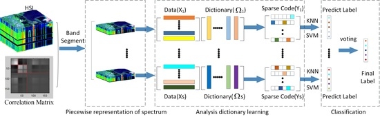
We use the characteristics of HSI data to model a new HSI oriented ADL model in this paper. The entire flowchart is shown in Figure 1. Given an HSI, we divide the high-dimensional spectrum h i R m the sensor captured into multiple segments to reduce the influence of nonlinearity within each spectrum on classification. Second, we build analysis dictionary model for each segment, where the relationships among the spectra are exploited to boost the discriminability of the generated codebook. Then, a voting strategy is used to obtain the final classification results.

2.2. Piecewise Representation of Spectrum

It is commonly realized that the difficulty of classification comes from class ambiguity, i.e., the sample variations come from within-class maybe larger than that from between-class. For HSI data, lots of factors will lead to class ambiguity, such as the nonlinearity of spectrum, pixel difference caused by different imaging conditions, etc. In this subsection, we pay our attention to nonlinearity of spectrum first.
Due to the nonlinearity of spectrum, directly model analysis dictionary on the entire spectrum h i R m the sensor captured is not a good choice, which also can be seen from the experimental results. Considering that piecewise linear representation [36] is a common strategy to deal with nonlinearity, we divide the high-dimensional spectrum h i into multiple segments first to address this problem. Then, we apply the analysis dictionary model for each segment independently.
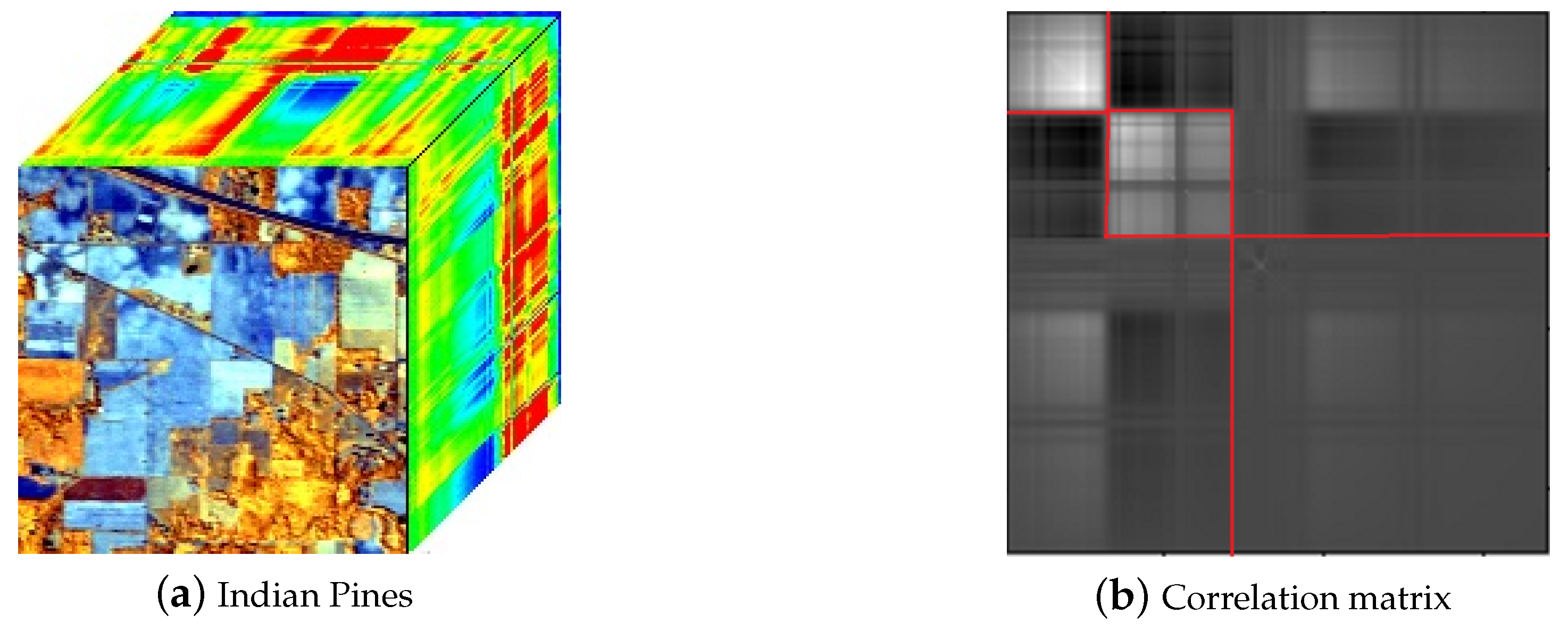
Different methods can be used to divide the spectrum into segments. Considering correlation within spectrum shows obvious block-diagonal structure, it is used to segment the spectrum in this paper [37]. Specifically, given H , we calculate the correlation matrix on spectral domain (i.e., the row direction of the matrix) as
C o r i , j = C o v i , j C o v i , i C o v j , j ,
where C o r ( i , j ) is the correlation coefficient between the i-th band and the j-th band of H . In Equation (3), C o v is the covariance matrix of H and is calculated by
C o v = E H E H H E H T .
In Equation (4), E · denotes the mathematical expectation. Figure 2 illustrates Indian Pines dataset and the generated correlation matrix obtained via Equation (3). In Figure 2, white color represents strong correlation while black color represents low correlation. More brighter, more corrleated. It can be seen from Figure 2 that block-diagonal structure exists in the generated correlation matrix, which justify the rationality of dividing the entire spectrum h i into segments. To simplify the representation, we use x i R m 1 to denote the generated segment in the following. It is noticeable that the correlation matrix is only used as an example to separate the spectrum. Other methods [38,39] can also be introduced to divide the spectrum into segments. However, this is not the focus of this paper.

2.3. Analysis Dictionary Learning Constrained with the Relationship of Spectra

By dividing the spectrum into segments, the nonlinearity problem of spectrum classification can be alleviated. We then construct analysis dictionary independently for each segment.
Equation (2) demonstrates a basic analysis dictionary learning method. Though it shows superiority over typical synthesis dictionary learning methods, it considers the spectrum individually without considering the relationship of spectra. However, such relationship is also an important characteristic of HSI. To take advantage of such characteristic, we propose a new analysis dictionary learning method inspired by discriminative analysis dictionary learning [35], which generate codebook with a triplet relation constraint. The constructed analysis dictionary model is given as follows.
min Ω , Y i = 1 n d i s t y i , Ω x i + λ 1 i = 1 n d i s t ( y i , z i ) λ 2 i = 1 n u = 1 n v = 1 n T i u , v d i s t ( y i , y u ) d i s t ( y i , y v ) + λ i = 1 n j = 1 n S i , j d i s t ( y i , y j ) s . t . Ω W y i 0 T 0 , y j 0 T 0 , y u 0 T 0 , y v 0 T 0 , i = 1 , 2 , , n , j = 1 , 2 , , n , u = 1 , 2 , , n , v = 1 , 2 , , n
In Formula (5), d i s t · represents a kind of measure. z i is the target code, which can be label of spectrum h i or other equivalent representation of the label. λ 1 , λ 2 and λ are weighting coefficients which control the relative importance of different constraints. The minimization problem consists of the following four terms.
(1) The first term is the fidelity term. Minimizing it can guarantee the obtained sparse coefficient matrix Y and the dictionary Ω will reconstruct segments X = x 1 , x 2 , , x n .
(2) The second term is the discriminability promoting term [35], with which the label information z i can be introduced to generate discriminative sparse code y i . Minimizing the second term can enforce segments from the same category to have similar sparse codes.
(3) The third term is the triplet relation preserving term [35,40], which aims to preserve the local triplet topological structure of X in the generated sparse representation Y , i.e., d i s t ( y i , y u ) d i s t ( y i , y v ) if d i s t ( x i , x u ) d i s t ( x i , x v ) . Ideal local topological structure preserving is to maximize i = 1 n u = 1 n v = 1 n T i u , v d i s t ( y i , y u ) d i s t ( y i , y v ) , which equals to minimize i = 1 n u = 1 n v = 1 n T i u , v d i s t ( y i , y u ) d i s t ( y i , y v ) in Formula (5). T i u , v is a supervised measure [35] which is defined as
T i u , v = T i u , v s i g n T i u , v , z i = z u z v T i u , v s i g n T i u , v , z i = z v z u T i u , v , o t h e r w i s e
T i u , v is the element in the u-th row and v-th column of matrix T i , which is calculated by d i s t ( x i , x u ) d i s t ( x i , x v ) . The sign function s i g n · is defined as
s i g n a = 1 , a < 0 0 , a = 0 + 1 , a > 0
(4) The fourth term is a weighted sparsity preserving term, which guarantees the generated sparse representations similar enough if their corresponding segments are similar. S i , j measures the similarity between segments, which is defined as
S i , j = 1 1 + e ( S A D ( x i , x j ) ) , S A D ( x i , x j ) = cos 1 x i T x j x i 2 · x j 2
It is noticeable that the third and fourth terms constrain the generated sparse representation from local structure perspective and pixel-pair perspective, which are mutual complemented. The effectiveness combing these two terms can be seen from the experimental results.
If we use a weight matrix W R n × n to replace T i u , v , the local topological structure preserving term can be reformulated [35] as
max Y i = 1 n u = 1 n v = 1 n T i u , v d i s t ( y i , y u ) d i s t ( y i , y v ) = min Y i = 1 n j = 1 n W i j d i s t ( y i , y j ) ,
where W i j = k = 1 n T i k , j . Then Equation (5) evolves to
min Ω , Y i = 1 n d i s t y i , Ω x i + λ 1 i = 1 n d i s t ( y i , z i ) + λ 2 i = 1 n j = 1 n W i , j d i s t ( y i , y j ) + λ i = 1 n j = 1 n S i , j d i s t ( y i , y j ) s . t . Ω W y i 0 T 0 , y j 0 T 0 , i = 1 , 2 , , n , j = 1 , 2 , , n
By merging the last two terms in Equation (10), we obtain
min Ω , Y i = 1 n d i s t ( y i , Ω x i ) + λ 1 i = 1 n d i s t ( y i , z i ) + λ 2 i = 1 n j = 1 n ( W i , j + ρ S i , j ) d i s t ( y i , y j ) s . t . Ω W y i 0 T 0 , y j 0 T 0 , i = 1 , 2 , , n , j = 1 , 2 , , n
where ρ = λ 2 λ . Considering correntropy induced metric (CIM) [35,41] is a robust metric, it is adopted as the distance measure d i s t · in this paper and calculate the distance between two given data y i and y j as
d i s t ( y i , y j ) = 1 exp y i y j 2 2 / σ 2 1 2
By optimizing Equation (11), we can obtain the dictionary as well as the sparse representation generated from each segment, with which we can predict the classification result for each segment. However, Equation (11) is a non-convex problem, which is hard to be optimized directly. Instead, a half-quadratic technique proposed in [35] is introduced to optimize Equation (11) in this paper. Specifically, by introducing auxiliary matrices P , Q , R R n × n into the optimization problem [35,42], Equation (11) can be sovled by iteratively optimize Ω , Y and P , Q , R until convergence. In the following, we only give the updating equation for these variables. We refer the readers to see [35] for the details of the optimization process.
Step 1: Fixing Y , P , Q , R , we update dictionary Ω by
Ω = Y P t X T X P t + λ 2 L t X T + λ 3 I 1 ,
where t is the iteration number, λ 3 is a Lagrange multiplier for Ω , and L is the Laplacian matrix of W + ρ S .
Step 2: Fixing Ω , P , Q , R , we update Y via
min y i y i P i i t Ω x i + λ 1 Q i i t z i P i i t + λ 1 Q i i t 2 2 s . t . y i 0 T 0
which can be solved easily by applying hard thresholding operation.
Step 3: Fixing Ω and Y , the auxiliary matrics P , Q , R are updated via
P i i t + 1 = exp ( y i t + 1 Ω t + 1 x i 2 2 σ 2 ) , Q i i t + 1 = exp ( y i t + 1 z i 2 2 σ 2 ) , R i j t + 1 = exp ( Ω t + 1 x i Ω t + 1 x j 2 2 σ 2 )

2.4. Classification via Different Segments

Once we obtain the sparse representation of each segment, i.e., y i , we then use it to predict the class label for each segment. To discriminate the class label of the entire spectrum (i.e., pixel), we denote the label of the segment as seg-label in this paper. Any kind of classifier can be adopted to predict the seg-label for each segment. Considering that the proposed method aims to generate discriminative feature, simple classifiers including k-NN and SVM are adopted only in this paper.
Suppose we divide the entire spectrum of one pixel into S segments, we obtain S seg-labels with the adopted classifier. Denote these seg-labels as l 1 , l 2 , , l S , where l i is the classification result from the i-th segment, we then predict the class label l f i n a l for the pixel based on
l f i n a l = v o t e l 1 , l 2 , , l S .
v o t e · is a voting function. It selects the class that appears most frequently for the test pixel.
In this papar, we divide the spectrum into three segments for simplification. We adopt a simple voting strategy. If at least two seg-labels are same, we assign pixel the same class with the one dominate the seg-labels. Otherwise, the seg-labels are different for three segments. In this case, among three seg-labels, we randomly assign a seg-label to the class of pixel.

3. Experiments

We conduct experiments on HSI datasets to demonstrate the effectiveness of the proposed method. In the following, we first introduce the HSI datasets we used in the experiments. We then compare the proposed method with some state-of-the-art dictionary-based methods. Finally, we discuss the performance of the proposed method varied with different settings for HSI classification.

3.1. Dataset Description

Three benchmark HSI datasets including Indian Pines dataset, Pavia University (PaviaU) dataset and Salinas Scene dataset are adopted to verify the proposed method [43,44].
Indian Pines Dataset: Indian Pines dataset was acquired by the Airborne Visible/Infrared Imaging Spectrometer (AVIRIS) sensor in north-western Indiana, USA. The spectral range of Indian Pines is from 400 to 2450 nm. We remove 20 water absorption bands and use the remaining 200 bands for experiments. The imaged scene has 145 × 145 pixels, among which 10,249 pixels are labeled. Class number of Indian Pines dataset is 16.
PaviaU Dataset: PaviaU dataset was acquired in Pavia University, Italy, by the Reflective Optics System Imaging Spectrometer. The spatial resolution of PaviaU dataset is 1.3 m, while the spectral range is from 430 to 860 nm. After removing 12 water absorption bands, we keep 103 bands from the original 115 bands for experiment. The imaged scene has 610×340 pixels, among which 42,776 pixels are labeled. Class number of PaviaU dataset is 9.
Salinas Scene Dataset: The Salinas scene dataset was collected in Salinas Valley, California, which has a continuous spectral coverage from 400 to 2450 nm. There are 512 × 217 pixels, among which 54,129 pixels were labeled and used for the experiment. After removing the water absorption bands, we keep the remaining 204 bands in the experiments. Class number of Salinas dataset is 16.

3.2. Comparison Methods and Experimental Setup

We denote the proposed method as Ours in this paper. Since the proposed method is a dictionary learning-based HSI classification method, we mainly compare the proposed method with the existing dictionary learning-based methods. To further testify the performance of the proposed method, we compare the proposed method with a state-of-the-art deep learning-based method, i.e., 3D convolutional neural network (3D-CNN) [17], and the method based on the spectrum h i without feature extraction, which is denoted as Ori in this paper. In addition, since both piecewise representation and spectra relationship contribute to the final classification result for the proposed method, we implement two special versions of Ours, termed Ours-Seg and Ours-Sim, to verify the influence of these two parts on classification. Ours-Seg only considers the piecewise representation of spectrum whereas Ours-Sim only exploits the relationship of spectra for classification.
The dictionary learning-based methods we compared including sparse representation-based classification (SRC) [30], dictionary learning with structured incoherence (DLSI) [34], label consistent k-singular value decomposition algorithm (LC-KSVD) [31], fisher judgement dictionary learning method (FDDL) [33], and discriminative analysis dictionary learning (DADL). SRC, DLSI, LC-KSVD and FDDL are synthesis dictionary model-based methods, whereas DADL and Ours are analysis dictionary model-based ones. In SRC, segmented spectrum are chosen as the dictionary direclty, while learned dictionaries are used for DLSI, LC-KSVD, FDDL, DADL and Ours.
We normalize the HSI data into the range of 0 to 1 via a min-max normalization method. Except 3D-CNN, which is an end-to-end classification method without dividing feature extraction and classifier, both k-NN and SVM are adopted for all other methods in the experiments to testify whether the proposed method is applicable to different classifiers. All codes of the comparing methods are implemented by the authors with tuned parameters for best performance. For the proposed method, λ 1 , λ 2 and ρ are optimized by cross-validation, which are set to 1, 1 and 0.05, respectively.
For all datasets, we empirically set the number of segments as 3 in the experiments. For Indian Pine dataset, the generated three segments are bands 1–30, bands 30–75, and bands 75–200. For PaviaU dataset, the generated three segments are bands 1–73, bands 73–75 and bands 75–103. While for Salinas dataset, the generated three segments are bands 1–40, bands 40–80 and bands 80–204.
Overall accuracy (OA), which defines the ratio of correctly labeled samples to all test samples, is adopted to measure HSI classification results.

3.3. Comparison with Other Methods

In this section, two experiments are conducted. First, we choose 20% samples from each class as the training set, based on which we then predict the class label of the test pixel for all methods. Second, we compare the performance of all methods with different amount of training samples.

Experimental Results with 20% Training Samples

The number of training and test samples for each dataset is given in Table 1, where 20% pixels are randomly sampled from all labeled data for training. Table 2, Table 3, Table 4, Table 5, Table 6 and Table 7 report the average classification results for all methods across 10 rounds of different sampling, from which we can obtain the following conclusions.
(1) Compared with the synthesis dictionary model-based methods, analysis dictionary model-based methods including DADL, Ours, Ours-Seg and Ours-Sim can obtain higher classficiation results, which demonstrate the effectiveness of analysis dictionary model-based methods for HSI classification.
(2) Compared with k-NN, the SVM classifier can obtain better classification results with the same feature, since k-NN is a simple classifier without training while SVM tune its parameters with training data. Ours with k-NN classifier has better classification results, compared with all synthesis dictionary model-based methods with SVM classifier. For example, on Indian Pines dataset, the classification accuracy of Ours is 87.98% when using k-NN classifier, whereas the highest classification of synthesis dictionary model-based methods (i.e., FDDL) is only 72.98% even given SVM classifier.
(3) Compared with DADL which only uses the local triplet topology, the classification performance of the proposed method increases a lot. For example, the classification accuracy for Ours and DADL with k-NN classifier is 87.98% and 72.5%, respectively. The improvement of Ours over DADL comes from the fact that we simultaneously model the piecewise representation and the pixel similarity. The conclusion can also be seen from the experimental results of Ours-Seg, Ours-Sim, Ours and DADL. By comparing Ours-Seg and DADL, we can find that the classification results can be increased when we divide the spectrum into segments. By comparing Ours-Sim and DADL, we can find that the classification results also can be improved when we model pixel similarity into dictionary learning. Though Ours-Seg and Ours-Sim can obtain better classification results compared with DADL, they still inferior to Ours regarding HSI classification ability, which demonstrates that both piecewise representation and spectra relationship is important for the proposed method.
(4) Compared with Ori which is based on the spectrum directly, Ours has better classification results, which demonstrates the effectiveness of the proposed method. More importantly, the classification performance of Ours is more stable on all datasets, compared with Ori. For example, with k-NN classifier, though the classification accuracy of Ori (86.29%) closes to that of Ours (88.38%) on Salinas dataset, there is a large difference between Ori (65.08%) and Ours (87.98%) on Indian Pines dataset.
(5) Compared with 3D-CNN, the accuracy of Ours is lower when using together with k-NN classifier. However, when using this together with the SVM classifier, Ours can obtain better classification results compared with 3D-CNN. This is because k-NN is a simple classifier without training while SVM and 3D-CNN tune their parameters with training data. Thus, the performance of k-NN inferiors to SVM and 3D-CNN. In addition, since 3D-CNN has large amount of parameters, its performance relies on large amount of training data. However, when given small amount of (e.g., 20%) training data as the propose method demands, 3D-CNN cannot be well trained, with which the classification accuracy of 3D-CNN inferiors to Ours with SVM classifier.
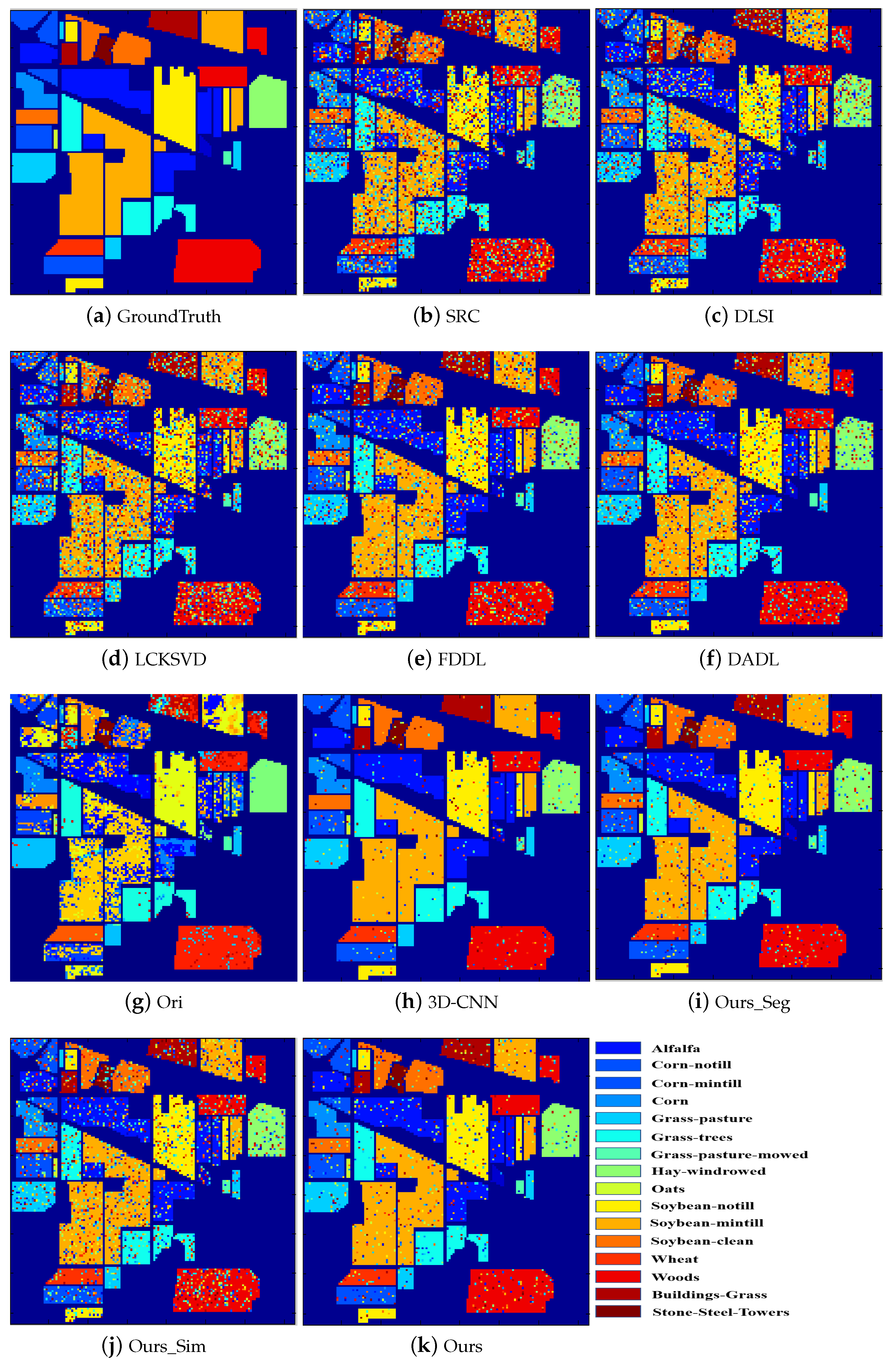
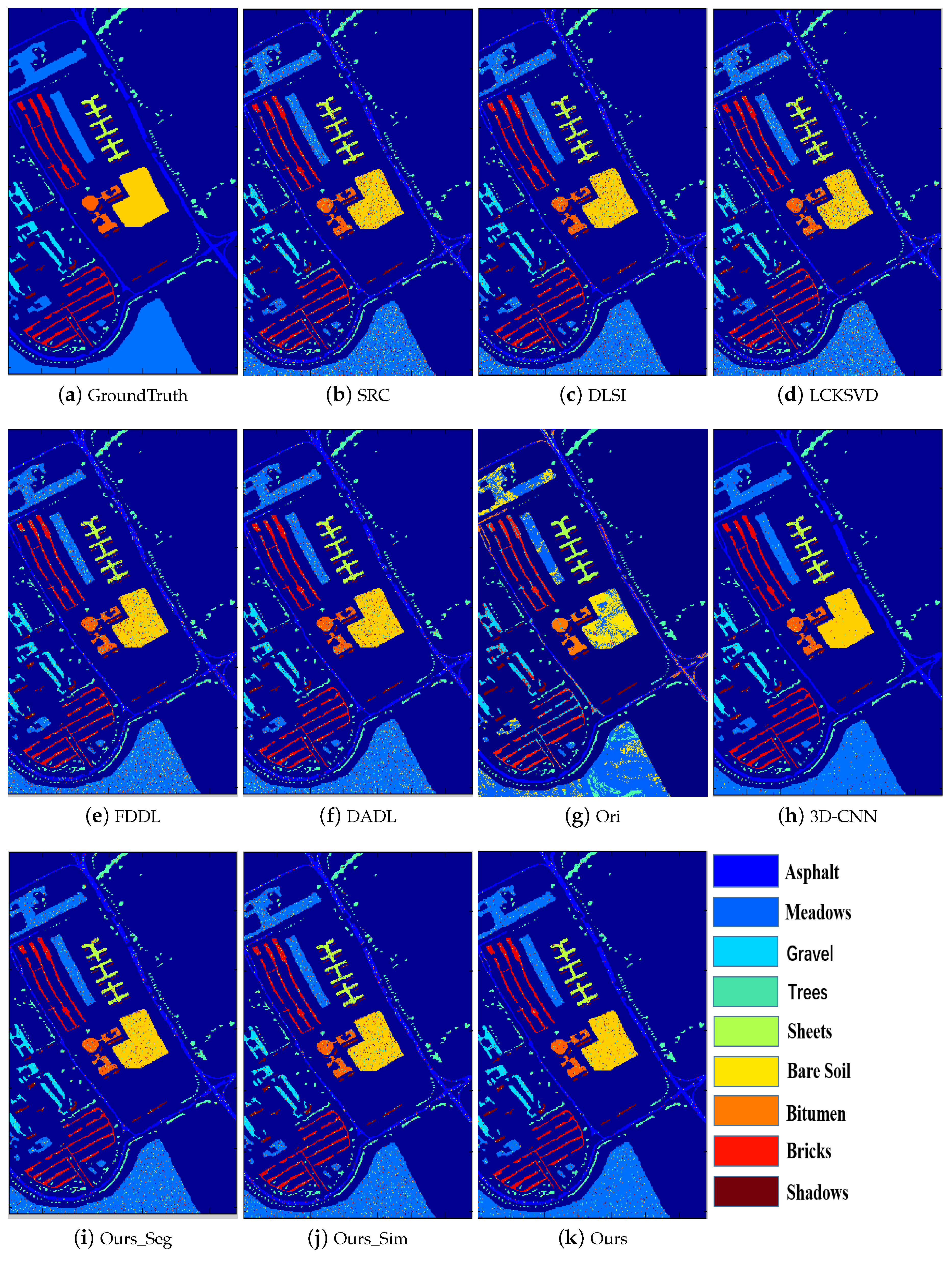
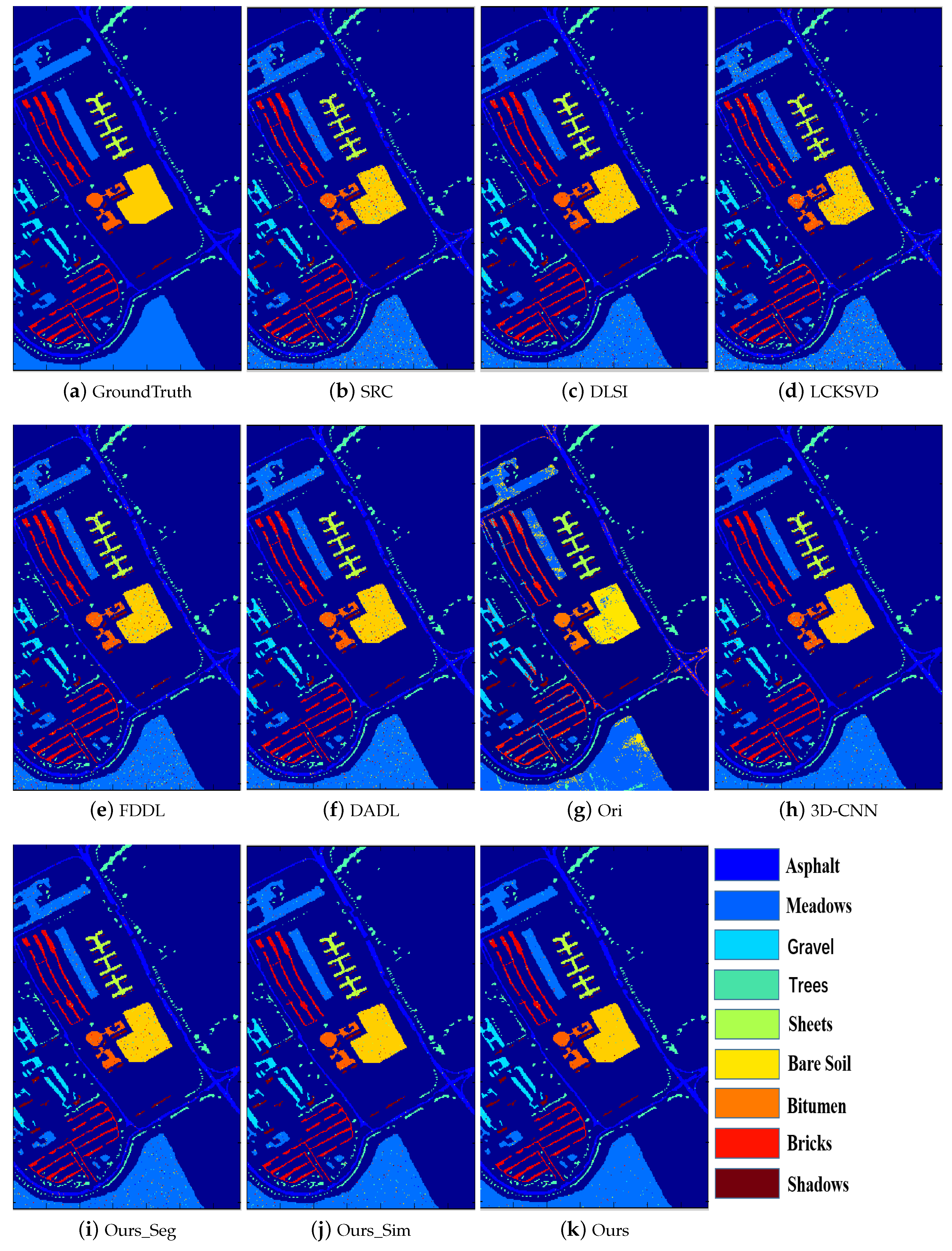
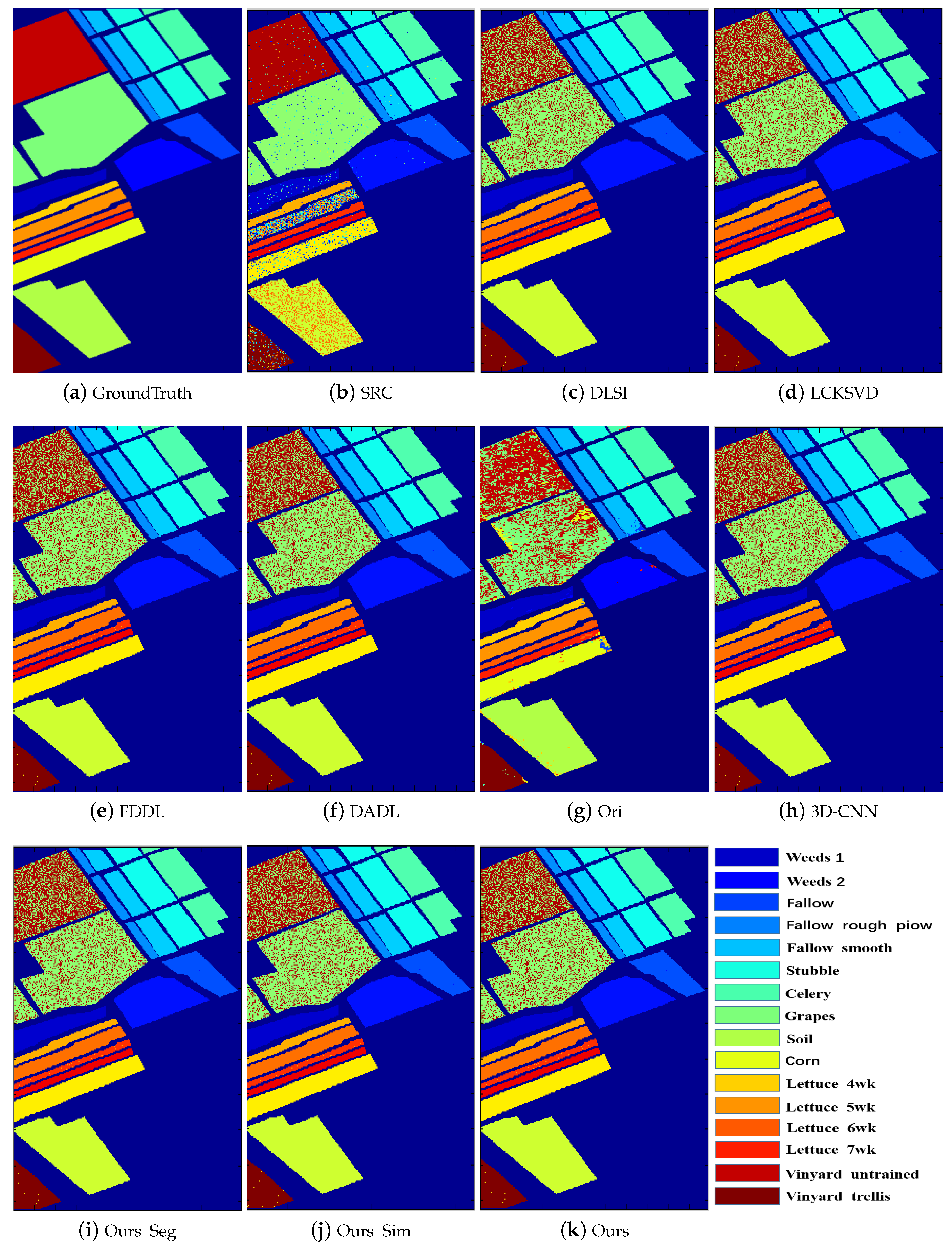
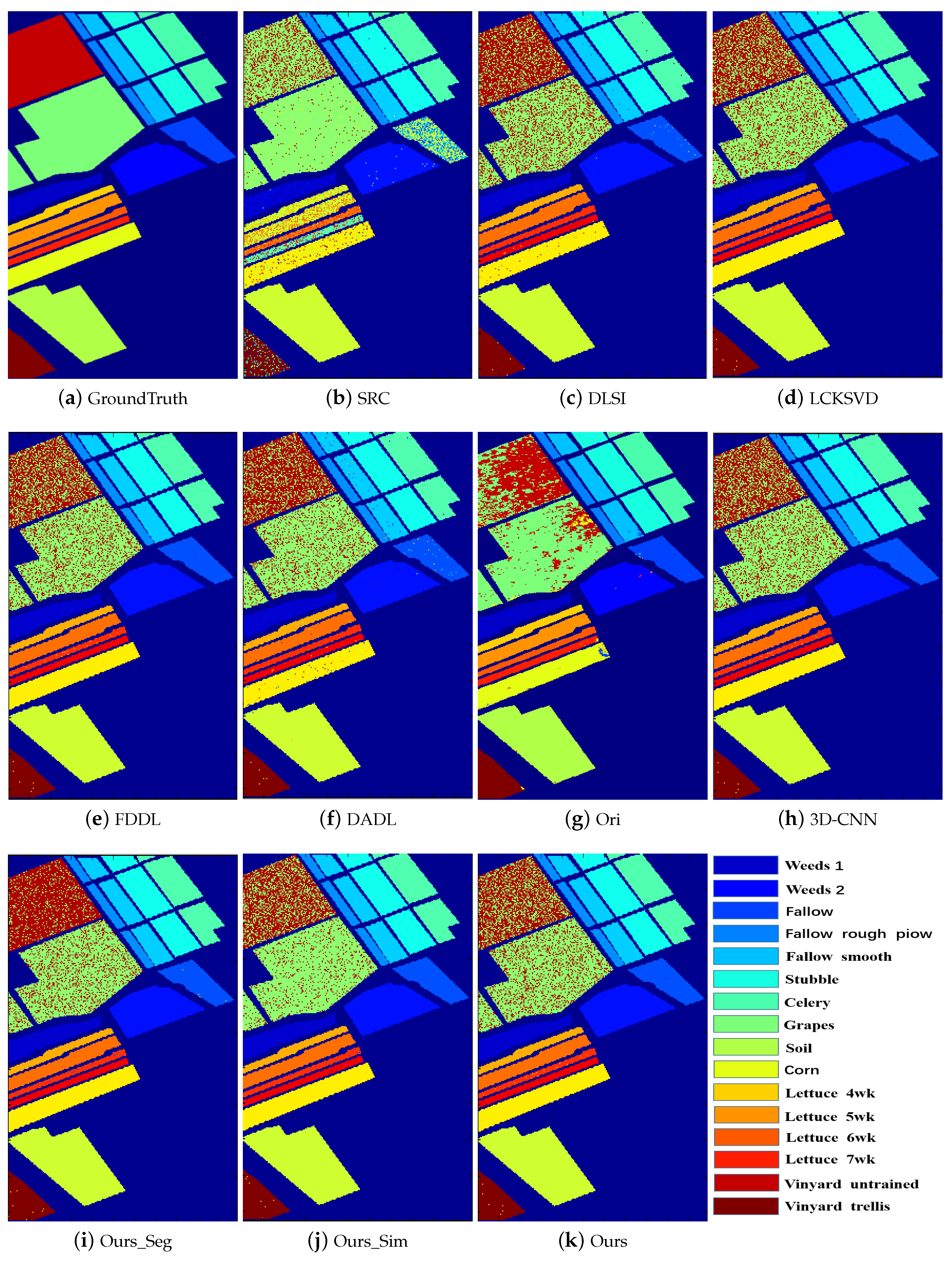
Figure 3, Figure 4, Figure 5, Figure 6, Figure 7 and Figure 8 illustrate the classification maps, where (a) represents the ground truth and (b)–(k) represent the results from different methods. In the classification map, we use a unique color to represent each category. From these figures, we can see that the proposed method with SVM classifier obtains more accurate and smoother results compared with the competing methods.

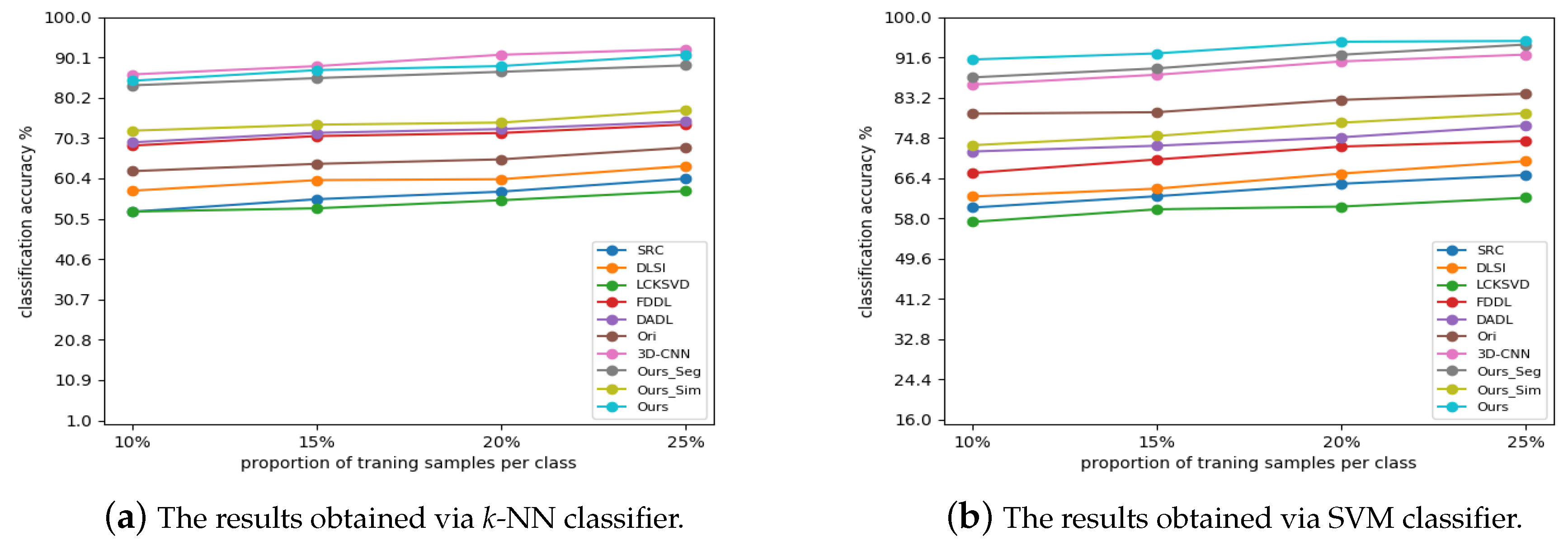
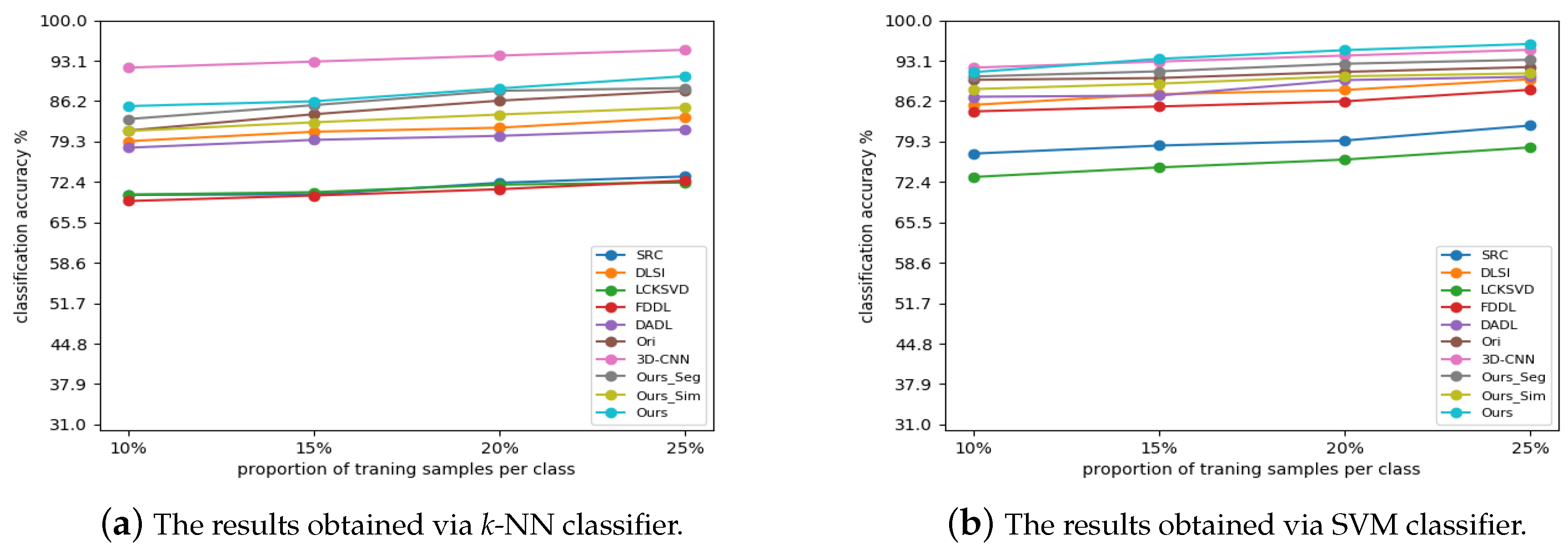
3.4. Experimental Results with Different Small Amount of Training Data

The classification results varied with the different small amount of training data are shown in Figure 9, Figure 10 and Figure 11, where the training data is varied from 10% to 25%. From the experimental results, we can see the classification results of the proposed methods increase when more samples are introduced for training, which is natural since classifier can be well trained with more training samples. Nevertheless, the proposed method outperforms all competing methods stably when using together with SVM classifier, and only inferiors to 3D-CNN when using together with k-NN classifier since k-NN is a classification method without training. The experimental results are inconsistent with that in Section 3.3. From the above results, we can conclude that the proposed method is effective for HSI classification.

4. Discussion

In the above experiments, we divide the entire spectrum into three segments, and then adopt a voting strategy to generate the final classification result. To testify the effectiveness of the adopted dividing and voting strategies, we compare it with the classification results directly obtained from each segment and the result from the entire spectrum. In the following, we use Seg-vote/Ours, Seg1, Seg2, Seg3 and Entire to denote the classification result from the dividing and voting strategy, the first segment, the second segment, the third segment and the entire spectrum, respectively. The experimental results are given in Table 8. We can observe that dividing and voting strategy can obtain better HSI classification results, compared with the segment or the entire spectrum-based method.

5. Conclusions

In the paper, we present a novel analysis dictionary learning model-based hyperspectral image classification method. The proposed framework naturally considers both the characteristics within the spectrum and among the spectra. By dividing the spectrum into several segments, the influence of strong nonlinearity with spectrum can be alleviated. In addition, the relationship among spectra can further improve the classification performance. Experimental results on three benchmark HSI datasets demonstrate the superiority of the proposed framework for HSI classification.

Author Contributions

W.W. and L.Z. conceived and designed the experiments; M.M. performed the experiments; W.W., P.Z., and Y.Z. analyzed the data; W.W., L.Z., M.M., and C.W. wrote the paper.

Funding

This research was funded by the National Natural Science Foundation of China (No. 61671385, 61571354, 61571362), the Natural Science Basis Research Plan in Shaanxi Province of China (No. 2017JM6021, 2018JM6015)

Conflicts of Interest

The authors declare no conflict of interest.

References

  1. Ghamisi, P.; Yokoya, N.; Li, J.; Liao, W.; Liu, S.; Plaza, J.; Rasti, B.; Plaza, A. Advances in Hyperspectral Image and Signal Processing: A Comprehensive Overview of the State of the Art. IEEE Geosci. Remote Sens. Mag. 2018, 5, 37–78. [Google Scholar] [CrossRef]
  2. Wei, W.; Zhang, L.; Jiao, Y.; Tian, C.; Wang, C.; Zhang, Y. Intra-Cluster Structured Low-Rank Matrix Analysis Method for Hyperspectral Denoising. IEEE Trans. Geosci. Remote Sens. 2019, 57, 866–880. [Google Scholar]
  3. He, L.; Li, J.; Liu, C.; Li, S. Recent Advances on Spectral-Spatial Hyperspectral Image Classification: An Overview and New Guidelines. IEEE Trans. Geosci. Remote Sens. 2018, PP, 1–19. [Google Scholar] [CrossRef]
  4. Guerra, R.; Barrios, Y.; Diaz, M.; Santos, L.; Lopez, S.; Sarmiento, R. A New Algorithm for the On-Board Compression of Hyperspectral Images. Remote Sens. 2018, 10, 428. [Google Scholar] [CrossRef]
  5. Zhang, L.; Wei, W.; Bai, C.; Gao, Y.; Zhang, Y. Exploiting Clustering Manifold Structure for Hyperspectral Imagery Super-Resolution. IEEE Trans. Image Process. 2018, 27, 5969–5982. [Google Scholar] [CrossRef] [PubMed]
  6. Fauvel, M.; Tarabalka, Y.; Benediktsson, J.A.; Chanussot, J.; Tilton, J.C. Advances in Spectral-Spatial Classification of Hyperspectral Images. Proc. IEEE 2013, 101, 652–675. [Google Scholar] [CrossRef]
  7. Camps-Valls, G.; Bruzzone, L. Kernel-based methods for hyperspectral image classification. IEEE Trans. Geosci. Remote Sens. 2005, 43, 1351–1362. [Google Scholar] [CrossRef] [Green Version]
  8. Wang, Q.; Lin, J.; Yuan, Y. Salient Band Selection for Hyperspectral Image Classification via Manifold Ranking. IEEE Trans. Neural Netw. Learn. Syst. 2016, 27, 1279–1289. [Google Scholar] [CrossRef]
  9. Rajadell, O.; García-Sevilla, P.; Pla, F. Spectral-Spatial Pixel Characterization Using Gabor Filters for Hyperspectral Image Classification. IEEE Geosci. Remote Sens. Lett. 2013, 10, 860–864. [Google Scholar] [CrossRef]
  10. Xiang, X.; Li, J.; Li, S. Multiview Intensity-Based Active Learning for Hyperspectral Image Classification. IEEE Trans. Geosci. Remote Sens. 2018, PP, 1–12. [Google Scholar]
  11. Blanzieri, E.; Melgani, F. Nearest Neighbor Classification of Remote Sensing Images with the Maximal Margin Principle. IEEE Trans. Geosci. Remote Sens. 2008, 46, 1804–1811. [Google Scholar] [CrossRef]
  12. Xue, Z.; Du, P.; Su, H. Harmonic Analysis for Hyperspectral Image Classification Integrated with PSO Optimized SVM. IEEE J. Sel. Top. Appl. Earth Observ. Remote Sens. 2014, 7, 2131–2146. [Google Scholar] [CrossRef]
  13. Sharma, S.; Buddhiraju, K.M. Spatial–spectral ant colony optimization for hyperspectral image classification. Int. J. Remote Sens. 2018, 39, 2702–2717. [Google Scholar] [CrossRef]
  14. Li, W.; Wu, G.; Zhang, F.; Du, Q. Hyperspectral Image Classification Using Deep Pixel-Pair Features. IEEE Trans. Geosci. Remote Sens. 2016, 55, 844–853. [Google Scholar] [CrossRef]
  15. Othman, E.; Bazi, Y.; Alajlan, N.; Alhichri, H.; Melgani, F. Using convolutional features and a sparse autoencoder for land-use scene classification. Int. J. Remote Sens. 2016, 37, 2149–2167. [Google Scholar] [CrossRef]
  16. Chen, Y.; Jiang, H.; Li, C.; Jia, X.; Ghamisi, P. Deep Feature Extraction and Classification of Hyperspectral Images Based on Convolutional Neural Networks. IEEE Trans. Geosci. Remote Sens. 2016, 54, 6232–6251. [Google Scholar] [CrossRef]
  17. Li, Y.; Zhang, H.; Shen, Q. Spectral–Spatial Classification of Hyperspectral Imagery with 3D Convolutional Neural Network. Remote Sens. 2017, 9, 67. [Google Scholar] [CrossRef]
  18. Fang, B.; Li, Y.; Zhang, H.; Chan, J.W. Hyperspectral Images Classification Based on Dense Convolutional Networks with Spectral-Wise Attention Mechanism. Remote Sens. 2019, 11, 159. [Google Scholar] [CrossRef]
  19. Zabalza, J.; Ren, J.; Yang, M.; Zhang, Y.; Wang, J.; Marshall, S.; Han, J. Novel Folded-PCA for improved feature extraction and data reduction with hyperspectral imaging and SAR in remote sensing. ISPRS J. Photogramm. Remote Sens. 2014, 93, 112–122. [Google Scholar] [CrossRef] [Green Version]
  20. Mura, M.D.; Villa, A.; Benediktsson, J.A.; Chanussot, J.; Bruzzone, L. Classification of Hyperspectral Images by Using Extended Morphological Attribute Profiles and Independent Component Analysis. IEEE Geosci. Remote Sens. Lett. 2011, 8, 542–546. [Google Scholar] [CrossRef]
  21. Nielsen, A.A. Kernel Maximum Autocorrelation Factor and Minimum Noise Fraction Transformations. IEEE Trans. Image Process. 2011, 20, 612–624. [Google Scholar] [CrossRef] [PubMed] [Green Version]
  22. Majdar, R.S.; Ghassemian, H. A probabilistic SVM approach for hyperspectral image classification using spectral and texture features. Int. J. Remote Sens. 2017, 38, 4265–4284. [Google Scholar] [CrossRef]
  23. Medjahed, S.A.; Saadi, T.A.; Benyettou, A.; Ouali, M. Gray Wolf Optimizer for hyperspectral band selection. Appl. Soft Comput. 2016, 40, 178–186. [Google Scholar] [CrossRef]
  24. Zhang, L.; Wei, W.; Zhang, Y.; Shen, C.; Hengel, A.V.D.; Shi, Q. Dictionary Learning for Promoting Structured Sparsity in Hyperspectral Compressive Sensing. IEEE Trans. Geosci. Remote Sens. 2016, 54, 7223–7235. [Google Scholar] [CrossRef]
  25. Gao, Q.; Lim, S.; Jia, X. Improved Joint Sparse Models for Hyperspectral Image Classification Based on a Novel Neighbour Selection Strategy. Remote Sens. 2018, 10, 905. [Google Scholar] [CrossRef]
  26. He, Z.; Wang, Y.; Hu, J. Joint Sparse and Low-Rank Multitask Learning with Laplacian-Like Regularization for Hyperspectral Classification. Remote Sens. 2018, 10, 322. [Google Scholar] [CrossRef]
  27. Zhang, L.; Wei, W.; Zhang, Y.; Shen, C.; van den Hengel, A.; Shi, Q. Cluster Sparsity Field: An Internal Hyperspectral Imagery Prior for Reconstruction. Int. J. Comput. Vis. 2018, 126, 797–821. [Google Scholar] [CrossRef]
  28. Rubinstein, R.; Bruckstein, A.M.; Elad, M. Dictionaries for Sparse Representation Modeling. Proc. IEEE 2010, 98, 1045–1057. [Google Scholar] [CrossRef] [Green Version]
  29. Zhang, S.; Zhang, M.; He, R.; Sun, Z. Transform-invariant dictionary learning for face recognition. In Proceedings of the IEEE International Conference on Image Processing, Paris, France, 27–30 October 2015; pp. 348–352. [Google Scholar]
  30. Wright, J.; Yang, A.Y.; Sastry, S.S.; Ma, Y. Robust Face Recognition via Sparse Representation. IEEE Trans. Pattern Anal. Mach. Intell. 2008, 31, 210–227. [Google Scholar] [CrossRef]
  31. Jiang, Z.; Lin, Z.; Davis, L.S. Learning a discriminative dictionary for sparse coding via label consistent K-SVD. Proc. IEEE Conf. Comput. Vis. Pattern Recognit. 2011, 42, 1697–1704. [Google Scholar]
  32. Kviatkovsky, I.; Gabel, M.; Rivlin, E.; Shimshoni, I. On the Equivalence of the LC-KSVD and the D-KSVD Algorithms. IEEE Trans. Pattern Anal. Mach. Intell. 2017, 39, 411–416. [Google Scholar] [CrossRef] [PubMed]
  33. Yang, M.; Zhang, L.; Feng, X.; Zhang, D. Fisher Discrimination Dictionary Learning for sparse representation. Proc. IEEE Int. Conf. Comput. Vis. 2011, 24, 543–550. [Google Scholar]
  34. Ramirez, I.; Sprechmann, P.; Sapiro, G. Classification and clustering via dictionary learning with structured incoherence and shared features. In Proceedings of the IEEE Conference on Computer Vision and Pattern Recognition, San Francisco, CA, USA, 13–18 June 2010. [Google Scholar]
  35. Guo, J.; Guo, Y.; Kong, X.; Zhang, M.; He, R. Discriminative Analysis Dictionary Learning. In Proceedings of the Thirtieth AAAI Conference on Artificial Intelligence, Phoenix, AZ, USA, 12–17 February 2016. [Google Scholar]
  36. Kiani, V.; Harati, A.; Vahedian, A. Planelets—A Piecewise Linear Fractional Model for Preserving Scene Geometry in Intra-Coding of Indoor Depth Images. IEEE Trans. Image Process. 2017, 26, 590–602. [Google Scholar] [CrossRef] [PubMed]
  37. Wang, C.; Zhang, L.; Wei, W.; Zhang, Y. When Low Rank Representation Based Hyperspectral Imagery classification Meets Segmented Stacked Denoising Auto Encoder Based Spatial-Spectral Feature. Remote Sens. 2017, 10, 284. [Google Scholar] [CrossRef]
  38. Kanungo, T.; Mount, D.M.; Netanyahu, N.S.; Piatko, C.D.; Silverman, R.; Wu, A.Y. An Efficient k-Means Clustering Algorithm: Analysis and Implementation. IEEE Trans. Pattern Anal. Mach. Intell. 2002, 24, 881–892. [Google Scholar] [CrossRef]
  39. Xiang, X.; Li, J.; Wu, C.; Plaza, A. Regional clustering-based spatial preprocessing for hyperspectral unmixing. Remote Sens. Environ. 2018, 204, 333–346. [Google Scholar]
  40. Luo, D.; Ding, C.H.Q.; Nie, F.; Huang, H. Cauchy Graph Embedding. In Proceedings of the International Conference on International Conference on Machine Learning, Bellevue, WA, USA, 28 June–2 July 2011; pp. 553–560. [Google Scholar]
  41. Ran, H.; Hu, B.-G.; Zheng, W.-S.; Kong, X.-W. Robust principal component analysis based on maximum correntropy criterion. IEEE Trans. Image Process. 2011, 20, 1485–1494. [Google Scholar] [CrossRef] [PubMed]
  42. Nikolova, M.; Ng, M. Analysis of Half-Quadratic Minimization Methods for Signal and Image Recovery; Society for Industrial and Applied Mathematics: Philadelphia, PA, USA, 2005; pp. 937–966. [Google Scholar]
  43. Zhang, L.; Zhang, Y.; Yan, H.; Gao, Y.; Wei, W. Salient Object Detection in Hyperspectral Imagery using Multi-scale Spectral-Spatial Gradient. Neurocomputing 2018, 291, 215–225. [Google Scholar] [CrossRef]
  44. Camps-Valls, G.; Gomez-Chova, L.; Munoz-Mari, J.; Vila-Frances, J.; Calpe-Maravilla, J. Composite kernels for hyperspectral image classification. IEEE Geosci. Remote Sens. Lett. 2006, 3, 93–97. [Google Scholar] [CrossRef]
Figure 1. The proposed architecture.
Remotesensing 11 00397 g001
Figure 2. Indian Pines dataset (a) and the generated spectral correlation matrix (b).
Remotesensing 11 00397 g002
Figure 3. Classification maps of different methods on the Indian Pines dataset via k-NN classifier (ak).
Remotesensing 11 00397 g003
Figure 4. Classification maps of different methods on the Indian Pines dataset via SVM classifier (ak).
Remotesensing 11 00397 g004
Figure 5. Classification maps of different methods on the PaviaU dataset via k-NN classifier (ak).
Remotesensing 11 00397 g005
Figure 6. Classification maps of different methods on the PaviaU dataset via SVM classifier (ak).
Remotesensing 11 00397 g006
Figure 7. Classification maps of different methods on the Salinas dataset via k-NN classifier (ak).
Remotesensing 11 00397 g007
Figure 8. Classification maps of different methods on the Salinas dataset via SVM classifier (ak).
Remotesensing 11 00397 g008
Figure 9. Classification performance with different numbers of training samples on Indian Pines dataset via k-NN (a) and SVM (b).
Remotesensing 11 00397 g009
Figure 10. Classification performance with different numbers of training samples on PaviaU dataset via k-NN (a) and SVM (b).
Remotesensing 11 00397 g010
Figure 11. Classification performance with different numbers of training samples on Salinas dataset via k-NN (a) and SVM (b).
Remotesensing 11 00397 g011
Table 1. Training and test numbers for three datasets (Indian Pines, PaviaU, Salinas) used in this paper.
No.Indiana PinesPaviaUSalinas
Class NameTrainTestClass NameTrainTestClass NameTrainTest
1Asphalt13275304Alfalfa937Brocoli_14021607
2Meadows373014,919Corn-notill2861142Brocoli_27452981
3Gravel4201679Corn-mintill166664Fallow3951581
4Trees6132451Corn47190Fallow_plow2791115
5Sheets2691076Grass-pasture97386Fallow_smooth5362142
6Bare Soil10064023Grass-trees146584Stubble7923167
7Bitumen2661064Grass-pasture-mowed622Celery7162863
8Bricks7352947Hay-windrowed96382Grapes22549017
9Shadows189758Oats416Soil_vinyard12414962
10Soybean-notill193779Corn_weeds6562622
11Soybean-minill4911964Lettuce_4wk214854
12Soybean-clean119474Lettuce_5wk3851542
13Wheats41164Lettuce_6wk183733
14Woods2521013Lettuce_7wk214856
15Bulidings-Grass77309Vinyard_un.14545814
16Stone-Steel-Towers1974Vinyard_ve.3611446
Sum855534,2212049820010,82743,302
Table 2. Classification accuracy (%) of different methods on the Indian Pines dataset via k-NN classifier. The highest accuracy in each row is boldfaced.
No.SRCDLSILC-KSVDFDDLDADLOri3D-CNNOurs_SegOurs_SimOurs
123.1622.2219.6614.5224.7035.4870.1551.4130.2261.26
282.5090.9693.8696.9388.2553.1796.1293.1992.9495.28
392.9290.9693.8694.1396.3157.6193.1995.9196.9296.12
464.7668.7061.0866.1284.4083.7894.1186.1073.2494.95
572.4794.5294.3385.2193.1290.4596.1297.1892.6095.97
695.8499.5995.8994.1094.0293.7797.1397.8197.1196.96
717.0414.2013.3014.8722.1884.6160.1443.1060.1557.13
885.9288.0290.6792.1090.1999.6490.1797.2897.4595.37
931.1030.4228.0630.1814.1720.0080.1232.2716.3751.00
1086.2190.7486.1788.0392.1074.3590.1296.2295.1096.07
1179.2379.7174.5477.2084.1151.4996.3694.2186.7996.24
1296.6795.9596.5075.2497.6252.9298.4397.3097.2096.23
1368.9562.8955.4073.9472.1280.0093.6784.1670.7290.11
1481.3485.3085.3088.5471.9281.9793.1786.8669.7291.51
1583.1080.8581.4886.1786.2245.1698.3688.9988.2497.64
1639.8940.0832.1735.5952.4683.3398.3168.1051.2187.11
OA57.1560.2055.0471.5572.565.0890.7586.5674.0687.98
Table 3. Classification accuracy (%) of different methods on the Indian Pines dataset via SVM classifier. The highest accuracy in each row is boldfaced.
No.SRCDLSILC-KSVDFDDLDADLOri3D-CNNOurs_SegOurs_SimOurs
120.2621.3218.4615.5425.7080.6670.1553.4932.6262.16
284.1089.2692.1697.8389.3578.7596.1294.8990.9097.48
393.6187.2692.4697.8395.2082.7093.1998.9698.9098.52
465.8370.2760.9867.3286.4094.5994.1189.1075.2495.95
573.6793.5195.3389.6194.5294.7096.1299.3893.6097.97
696.4498.1993.8997.4097.1296.0497.1399.8698.9198.36
713.5419.4015.3015.9718.1861.5460.1445.1320.6052.83
888.5285.1287.2792.2891.3998.5690.1799.3898.1596.37
928.0035.3229.0633.9812.27100.0080.1230.7715.8750.00
1089.8187.3486.1786.2393.2082.9090.1297.4292.9099.07
1178.5381.7173.1478.7085.2172.7396.3695.2387.9997.84
1298.1791.9593.5076.7498.6791.3598.4399.5098.5099.83
1361.7568.8954.2074.5471.92100.0093.6786.8669.7291.51
1482.1483.3782.1388.5471.9290.4293.1786.8669.7291.51
1582.8083.1581.2888.1287.9282.8098.3190.3989.1499.74
1636.8045.0836.278.5950.4689.7487.2369.0050.8186.91
OA65.2267.3560.4672.9874.9282.7290.7592.1477.9794.86
Table 4. Classification accuracy (%) of different methods on the PaviaU dataset via k-NN classifier. The highest accuracy in each row is boldfaced.
No.SRCDLSILC-KSVDFDDLDADLOri3D-CNNOurs_SegOurs_SimOurs
195.2995.9995.2395.1197.0271.5098.3297.0497.9197.56
287.7989.5387.1589.0790.0176.3996.0292.4792.3195.65
382.8686.2082.6783.9985.2978.7993.1888.9487.4293.29
492.0693.2489.3891.1092.9094.8095.1294.7794.4897.39
569.8774.0269.3771.7775.6999.1386.7980.4978.2085.45
699.8098.9898.4398.6599.6075.1597.1799.5699.9299.56
769.5673.2771.2372.4076.0091.5088.1279.6478.2486.64
896.6494.9294.2196.3696.9278.4698.2796.5996.9697.12
962.4363.7759.3363.0464.8199.8785.8972.9070.5681.21
OA79.2381.3778.0480.2581.5178.5394.1688.4084.1290.52
Table 5. Classification accuracy (%) of different methods on the PaviaU dataset via SVM classifier. The highest accuracy in each row is boldfaced.
No.SRCDLSILC-KSVDFDDLDADLOri3D-CNNOurs_SegOurs_SimOurs
196.0992.1992.1391.9196.1283.3898.3296.2498.9198.96
288.3987.2390.3592.2792.2193.2596.0290.1793.4196.15
383.6693.7084.2785.1986.8984.0493.1890.1490.7294.69
490.0690.6482.1893.4091.4096.4495.1295.1795.2895.09
574.2782.4273.8778.1778.1999.3986.7982.9980.2088.15
695.8095.1894.7395.6197.2092.1397.1796.9698.1297.24
776.1679.9779.5376.1079.2094.8688.1280.8479.7489.14
894.6491.9290.2193.1695.1287.2498.2797.2995.4698.92
967.4370.7769.3373.0470.8187.1985.8975.7873.2686.11
OA88.6090.2085.3489.5090.3791.1994.1692.7693.8095.21
Table 6. Classification accuracy (%) of different methods on the Salinas dataset via k-NN classifier. The highest accuracy in each row is boldfaced.
No.SRCDLSILC-KSVDFDDLDADLOri3D-CNNOurs_SegOurs_SimOurs
191.7999.0098.6398.2098.3897.9099.75100.0099.75100.00
299.0699.6399.2699.5399.5399.46100.0099.9099.7799.93
399.2499.4398.4898.9997.0398.9999.9498.6198.2398.55
499.4698.4897.4998.3098.2199.7599.5599.8299.4699.91
599.0798.5598.0498.4196.3696.2199.1199.4099.2199.44
699.8499.6299.2799,5399.7299.6399.84100.0099.87100.00
799.6999.5899.2099.4899.5198.85100.00100.0099.86100.00
896.1366.1666.0466.1376.0864.4865.6384.5684.5284.57
9100.0099.6299.4099.5699.5296.6499.8699.6499.5699.66
1077.2799.2198.7799.0999.2190.2599.6899.2599.0999.29
1197.4298.3697.0798.0196.8494.2499.7792.5192.0492.62
1215.2499.3598.6499.1698.5199.94100.0099.94100.00100.00
1398.3695.0894.8295.9197.8296.6597.9599.5999.6899.73
1498.2598.4897.2098.1396.7393.4599.8899.4299.9599.53
1511.0167.3467.1567.2966.5369.4567.5470.3370.2670.61
1678.9198.6997.8698.4198.5598.1399.38100.0099.72100.00
OA72.2781.6771.9579,1780.2886.2993.9887.9783.9288.38
Table 7. Classification accuracy (%) of different methods on the Salinas dataset via SVM classifier. The highest accuracy in each row is boldfaced.
No.SRCDLSILC-KSVDFDDLDADLOri3D-CNNOurs_SegOurs_SimOurs
198.5099.4498.6399.2698.9499.3999.75100.00100.00100.00
299.2999.8799.4399.7699.8399.71100.0099.9799.97100.00
399.6899.8798.9299.4397.6099.2799.9499.8198.6199.87
4100.0099.1098.0398.9299.0199.5099.5599.73100.00100.00
599.3998.8898.2798.7496.7896.8599.1199.4499.4999.63
6100.0099.8499.4399,75100.0099.7399.84100.00100.00100.00
799.9399.8399.3799.7299.8399.62100.00100.00100.00100.00
896.2166.2466.1066.2176.1882.3865.6386.0287.9184.62
999.7899.7699.5099.7099.7098.2399.8699.9099.6899.74
1078.5599.4898.9799.3799.5693.4099.6899.8499.3399.44
1198.2499.1897.6698.8397.8998.1599.7795.0892.7493.09
1215.7099.8198.9699.6199.0999.77100.0098.51100.00100.00
1399.3297.2795.5096.8699.0599.4497.9597.8199.86100.00
1499.0799.3097.7898.9597.7898.7499.8896.7399.56100.00
1511.1367.4667.2367.3066.6871.2867.5475.1370.4370.61
1679.3999.1098.2098.8999.1799.0799.38100.00100.00100.00
OA79.4888.1076.2386.1789.8091.2093.9892.5990.4594.91
Table 8. Classification accuracy(%)on three datasets with different segments used.
ClassifierPaviaU
Seg1Seg2Seg3Seg-voteEntire
k-NN72.1780.7484.3590.5284.12
SVM82.6791.3492.8995.2193.80
ClassifierIndian Pines
Seg1Seg2Seg3Seg-voteEntire
k-NN69.2372.7073.0887.9874.06
SVM70.1576.5077.1294.8677.97
ClassifierSanlinas
Seg1Seg2Seg3Seg-voteEntire
k-NN74.5679.7684.0788.3883.92
SVM83.6787.689.1794.9190.45

