Article

Infrared Small Target Detection Based on Partial Sum of the Tensor Nuclear Norm

1
School of Information and Communication Engineering, University of Electronic Science and Technology of China, Chengdu 611731, China
2
Center for Information Geoscience, University of Electronic Science and Technology of China, Chengdu 611731, China
*
Author to whom correspondence should be addressed.
Remote Sens. 2019, 11(4), 382; https://doi.org/10.3390/rs11040382
Submission received: 12 January 2019 / Revised: 4 February 2019 / Accepted: 11 February 2019 / Published: 13 February 2019
(This article belongs to the Special Issue Remote Sensing for Target Object Detection and Identification)

Abstract

:
Excellent performance, real time and strong robustness are three vital requirements for infrared small target detection. Unfortunately, many current state-of-the-art methods merely achieve one of the expectations when coping with highly complex scenes. In fact, a common problem is that real-time processing and great detection ability are difficult to coordinate. Therefore, to address this issue, a robust infrared patch-tensor model for detecting an infrared small target is proposed in this paper. On the basis of infrared patch-tensor (IPT) model, a novel nonconvex low-rank constraint named partial sum of tensor nuclear norm (PSTNN) joint weighted l1 norm was employed to efficiently suppress the background and preserve the target. Due to the deficiency of RIPT which would over-shrink the target with the possibility of disappearing, an improved local prior map simultaneously encoded with target-related and background-related information was introduced into the model. With the help of a reweighted scheme for enhancing the sparsity and high-efficiency version of tensor singular value decomposition (t-SVD), the total algorithm complexity and computation time can be reduced dramatically. Then, the decomposition of the target and background is transformed into a tensor robust principle component analysis problem (TRPCA), which can be efficiently solved by alternating direction method of multipliers (ADMM). A series of experiments substantiate the superiority of the proposed method beyond state-of-the-art baselines.

Graphical Abstract

1. Introduction

Infrared small target detection is of great importance in many military applications, such as early-warning systems, missile-tracking systems, and precision guided weapons. Unfortunately, infrared small target detection is still full of challenges, which is mainly related to the following. Firstly, because of the long imaging distance, small target is often spot-like, lacking texture and structural information; secondly, infrared imaging is also influenced by complex backgrounds, clutters, and atmospheric radiation, resulting in low signal-to-clutter (SCR) ratio in infrared images, and sometimes the target is even submerged by the background; thirdly, interferences such as artificial buildings, ships in the sea and birds in the sky also have a bad impact on detection ability. How to effectively suppress the background, improve the detection ability of the target, and reduce false alarms have always been difficult problems to solve.
In general, infrared small target detection methods can be divided into two categories: sequential-based and single-frame-based methods. Traditional sequential-based methods including pipeline filtering [1], 3D matched filtering [2], and multistage hypothesis testing [3] are applicable when the background is static and homogeneous, utilizing both spatial and temporal information to capture the target trajectory. However, in real applications, the movement between the target and imaging sensor is fast, coupled with various complex backgrounds, the performance of sequential-based methods degrades rapidly. Besides, those methods are unable to meet the real-time requirements due to the usage of multiple frames. Although there are still some studies on sequential-based methods [4,5], single-frame-based methods have attracted more research attention in recent years [6,7,8].
The prior information is the key to the success of single-frame-based methods, also in many other fields [9,10,11]. Up to now, the consistency of backgrounds [12,13,14,15], the saliency of targets [16,17,18,19], the sparsity of targets and the low rank of backgrounds [20,21,22,23,24] are the most used assumptions to detect infrared small targets in single image from different perspectives. The former two are local priors, whereas the latter two are nonlocal priors which are usually exploited simultaneously. Under simple scenes, the local priors are enough to distinguish target from background. Nevertheless, most real scenes are complex, which greatly limits the application of local priors. The nonlocal priors are more powerful and fit the real scenes well but still suffer from the sparse edges and noise. In fact, the combination of two types of prior information can improve the detection performance. Therefore, a suitable model for incorporating the local and nonlocal prior information plays a vital role in realizing high-efficiency detection methods.

1.1. Related Works on Single-Frame-Based Infrared Small Target Detection

According to the usage of prior information, the single-frame-based approaches can be mainly classified into two groups: filtering methods using local priors and optimizing methods using nonlocal priors. The first type of filtering methods exploits filters to estimate the background based on the prior information of background consistency. The target is enhanced by subtracting the predicted background from the original image. Conventional typical filters including Top-hat filter [12], two-dimensional least mean square (TDLMS) filter [15], and Max-mean filter [13] can catch the target easily under simple uniform scenes. Unfortunately, these filters cannot handle complex scenes full of edges and interferences well. In order to overcome this disadvantage, many improved filter were developed [25,26,27,28]. Another type of filtering methods highlights the small target based on the human visual system (HVS) via the calculation of saliency map. The contrast between target and its local neighborhood is a common measure to obtain the saliency map. Many HSV-based approaches such as Laplacian of Gaussian (LoG) filter [29], difference of Gaussian (DoG) filter [30], local contrast measure (LCM) [16], relative local contrast measure (RLCM) [19], multiscale patch-based contrast measure (MPCM) [31], weighted local difference measure (WLDM) [32], and multiscale gray and variance difference (MGVD) [33] measure were raised gradually. There are also methods to analyze visual saliency in the Fourier domain [34,35].
Unlike the filtering methods, optimizing methods employ the nonlocal self-correlation of infrared background and the sparsity of the target to reveal the data inner structure, which have been developed rapidly within the past decade. Assuming that the background comes from a single low-rank subspace, infrared patch image (IPI) model [20] regards the target as an outlier, so that the conventional target detection problem is converted to a robust principle component analysis (RPCA) [36] optimization problem. Compared with the traditional baselines, the detection ability has been significantly improved. Two obvious shortcomings of IPI are target over-shrinking and noise residuals mainly because of the low-rank regularization term which utilizes the nuclear norm. Subsequently, following this direction, more low-rank matrix recovery techniques were introduced into IPI model to get a better performance [21,37,38,39]. Considering that the original data are drawn from a union of low-rank subspaces, methods based on dictionary learning and sparse representation were proposed [24,40,41]. Unfortunately, either generating artificially or learning desired dictionaries to adapt to most scenarios is not easy but complex, especially when more dictionaries are needed. To dig out more useful information from the nonlocal configuration in patch space, Dai et al. [42] firstly generalized the IPI model to a novel infrared patch-tensor (IPT) model with the assumption that all the unfolding matrices are low rank, resulting in improved detection ability and reduction of computation time.

1.2. Motivation

For infrared small target detection, real-time processing and excellent performance are two fundamental expectations. However, one of the biggest problems of existing approaches is the imbalance between time and performance. Table 1 shows the computation time and performance of eight representative methods which concludes from our previous work [39]. Note that the time is obtained from processing an image of 256×200 pixels, and the full score of performance is five, the higher, the better. From Table 1, we can observe that the three filtering methods are fast but poor in performance, because of the simple assumptions regarding either the background or target. On the contrary, the six optimizing methods can obtain high-quality detection results but they are time consuming. The framework of optimization brings complex calculation and accurate detection results at the same time. How to simplify the calculation steps without destroying the detection performance is a crucial issue.
Experiments had shown the superiority of the RIPT model compared with state-of-the-art approaches (please see details in Ref. [42]). The intrinsic reasons lie in two aspects; for one thing, the novel patch-tensor model can extract more spatial correlations to reduce the interference, which is named the rare structure effect; for another, utilizing both local and nonlocal priors simultaneously increases the robustness of the RIPT upon various scenes and noise, as they are complementary when dealing with infrared small target detection. Nevertheless, the singleton model [43] used in RIPT may lead to a suboptimal value, since the sum of nuclear norms (SNN) [44] is not the convex envelope of the corresponding sum of ranks [45]. Furthermore, RIPT takes the difference of two eigenvalues derived from the structure tensor for the involvement of the local prior. The local structure weight map is illustrated in Figure 1, from which we can easily obtain the background edge information. An unfortunate fact worth mentioning is that the edge of the target is also highlighted. More specifically, it means the target would be over-shrunk, especially when the target lies upon boundaries such as those in Figure 1a, or there are no clear edges but the target is similar to that in Figure 1b. RIPT considers the background-related prior while ignoring the target-related prior since both of them can cause false alarms.
Inspired by the RIPT, the patch-tensor model can be exploited to seek out more intrinsic priors from a higher dimension. Another key factor is that RIPT with an additional stopping criterion is much faster than IPI. Hence, to alleviate the issue of imbalance and to overcome the two deficiencies of RIPT, this paper mainly makes three contributions.
  • First, to avoid the problem of equal treatment on singular values and reduce some biases, we develop a nonconvex infrared small target detection model based on partial sum of tensor nuclear norm (PSTNN), which can approximate the tensor rank better, and convert the detection task into a problem of solving the tensor robust principle component analysis model.
  • Second, by introducing the local prior which relates to background and target simultaneously as the local weight map, coupled with the reweighted scheme, thus the proposed model can preserve the target and suppress the background better, which assists us to complete the infrared small target detection task with good performance.
  • Third, an efficient algorithm based on the alternating direction method of multipliers (ADMM) is designed for solving the proposed model accurately. Meanwhile, with the help of tensor singular value decomposition (t-SVD) and an extra stopping condition, the algorithm complexity and computation time are dramatically reduced, leading to a faster speed in comparison with similar state-of-the-art methods.
The rest of this paper is structured as follows. Some related notations and preliminaries about tensor and mathematical theorems are introduced in Section 2. In Section 3, the construction of local prior map and proposed model are described in detail, and the ADMM solver to the optimization problem is also provided. Extensive experiments on various scenes and sequences are conducted to verify the effectiveness of the proposed method in Section 4. Section 5 and Section 6 present the discussion and conclusion of this paper, respectively.

2. Notations and Preliminaries

We first briefly introduce some necessary notions and preliminaries. In this paper, a tensor is denoted as X , a matrix is denoted as X , a vector is denoted as x , and a scalar is denoted as x . A fiber is a vector obtained by fixing every index of X but one, a slice is a matrix obtained by fixing every index of X but two. For a three-order X n 1 × n 2 × n 3 , its (i, j, k)-th entry is denoted as x i j k , and we use X i : : , X : i : , and X : : i respectively representing the i-th horizontal, lateral and frontal slice. In most cases, the i-th frontal slice X i : : is alternatively denoted as X ( i ) . The mode-i unfolding of X denoted by X ( i ) is composed by taking the mode-i fibers as its columns, which is also known as matricization or flattening. We define the operator unfold that maps X to a matrix, namely, X ( i ) = u n f o l d i ( X ) , and its inverse operator is fold. Besides, there are many acronyms used in this paper; we give a summary of these in Table 2 (excluding the acronyms of the comparison methods).

2.1. Tensor Singular Value Decomposition

For a three-order X n 1 × n 2 × n 3 , we denote X ¯ n 1 × n 2 × n 3 as the result of DFT along its third dimension by using the matlab command fft, i.e., X ¯ = f f t ( X , [ ] , 3 ) . The inverse operator ifft computes X from X ¯ , i.e., X = i f f t ( X ¯ , [ ] , 3 ) .
Definition 1.
(tensor conjugate transpose) [47] The conjugate transpose of a tensor X n 1 × n 2 × n 3 is the tensor X T n 1 × n 2 × n 3 obtained by conjugate transposing each of the frontal slice and then reversing the order of transposed frontal slices 2 through n 3 :
( X T ) ( 1 ) = ( X ( 1 ) ) T             a n d ( X T ) ( i ) = ( X ( n 3 + 2 i ) ) T ,           i = 2 , , n 3
Definition 2.
(identity tensor) [47] The identity tensor n 1 × n 2 × n 3 is the tensor with its first frontal slice being the n × n identity matrix, and the other frontal slices being all zeros.
Definition 3.
(orthogonal tensor) [47] A tensor Q n 1 × n 2 × n 3 is orthogonal if it satisfies
Q T Q = Q Q T
Definition 4.
(f-diagonal tensor) [47] A tensor X is called f-diagonal if each frontal slice X ( i ) is a diagonal matrix.
Theorem 1.
(t-SVD) [47] Let X n 1 × n 2 × n 3 . Then it can be factorized as
X = U S V T
where U n 1 × n 1 × n 3 , V n 2 × n 2 × n 3 are orthogonal tensors, and S n 1 × n 2 × n 3 is an f-diagonal tensor.
The illustration of t-SVD decomposition of an n 1 × n 2 × n 3 tensor is in Figure 2. Note that t-SVD can be obtained via computing matrix SVDs in the Fourier domain. An efficient and fast way to compute t-SVD is shown in Algorithm 1 [52].
Algorithm 1 T-SVD for three-order tensors
Input: X n 1 × n 2 × n 3
Output: T-SVD components U , S and V of X .
1. Compute X ¯ = f f t ( X , [ ] , 3 )
2. Compute each frontal slice of U ¯ , S ¯ and V ¯ from X ¯ by
for i = 1 , , ( n 3 + 1 ) / 2 do
   [ U ¯ ( i ) , S ¯ ( i ) , V ¯ ( i ) ] = SVD ( X ¯ ( i ) ) ;
end for
for i = ( n 3 + 1 ) / 2 + 1 , , n 3 do
   U ¯ ( i ) = conj ( U ¯ ( n 3 - i + 2 ) ) ;
   S ¯ ( i ) = S ¯ ( n 3 - i + 2 ) ;
   V ¯ ( i ) = c o n j ( V ¯ ( n 3 - i + 2 ) ) ;
end for
3. Compute U = ifft ( U ¯ , [ ] , 3 ) , S = ifft ( S ¯ , [ ] , 3 ) , and V = ifft ( V ¯ , [ ] , 3 ) .

2.2. Some Mathematical Preliminaries

Theorem 2.
(soft thresholding operator) [53] Let τ > 0 and X , Y n 1 × n 2 , define a l 1 norm minimization problem as
argmin X     τ X 1 + 1 2 X Y F 2
Then, Equation (4) could be solved by an elementwise soft thresholding operator defined as
S τ ( x ) = sign ( x ) × max ( | x | τ , 0 )
Definition 5.
(partial sum of singular values, PSSV) [50] For a matrix X n 1 × n 2 , the PSSV is defined as X p = N = i = p + 1 m i n ( n 1 , n 2 ) σ i ( X ) , where σ i ( X ) ( i = 1 , , m i n ( n 1 , n 2 ) ) is the i-th largest singular value of X, and N is the preserved target rank.
Theorem 3.
(partial singular value thresholding operator, PSVT) [50] Let τ > 0, l = min ( n 1 , n 2 ) and X , Y n 1 × n 2 which can be decomposed by SVD. Y can be considered as the sum of two matrices, Y = Y 1 + Y 2 = U Y 1 D Y 1 V Y 1 H + U Y 2 D Y 2 V Y 2 H , where U Y 1 , V Y 1 are the singular vector matrices corresponding to the N largest singular values, and U Y 2 , V Y 2 from the (N+1)-th to the last singular values. Define a complex minimization problem for PSSVas
argmin X   τ X p = N + β 2 X Y F 2
Then, the optimal solution of Equation (6) can be expressed by the PVST operator, which is defined as:
P N , τ ( Y ) = U Y ( D Y 1 + S τ [ D Y 2 ] ) V Y H = Y 1 + U Y 2 S τ [ D Y 2 ] V Y 2 H
where τ = λ / β , D Y 1 = diag ( σ 1 Y , , σ N Y , 0 , , 0 ) , and D Y 2 = diag ( 0 , , 0 , σ N + 1 Y , , σ l Y ) .

3. Proposed Method

Overall, an infrared image with small target can be described as follows [14]:
f D = f B + f T + f N
where f D , f B , f T denotes the original image, background image, target image respectively, and f N stands for the noise component. Depending on whether concentrating on merely the background, merely the target, or both of them leads to different methods to detect infrared small target. Unlike the general infrared image model, Gao et al. [20] generalized the traditional model into the IPI model, which can be formulated as
D = B + T + N
where D , B , T and N correspond to patch images of the original image, background image, target image and random noise, all of which are constructed by vectorizing the matrix within the sliding window. Since the infrared background is regarded as slowly transitional, that means that many local patches are approximately linearly correlated with each other. In other words, the configuration of nonlocal self-correlation leads to a low-rank background patch image. Besides, the small target only occupies a few pixels with respect to the whole image; thus the target patch image can be considered as a sparse matrix. Then, to separate the background and target is to solve an RPCA problem of recovering low-rank and sparse matrices. In terms of data dimensionality reduction and representation, the most popular method is PCA [54]. Recently, many other approaches spring up [36,55], and RPCA is an improvement of traditional PCA.

3.1. Infrared Patch-Tensor Model

To dig out more correlations among different patches, Dai et al. [42] proposed a novel target-background separation framework named the infrared patch-tensor model (IPT) based on a slightly different idea of construction. Transforming the original infrared image into a tensor is the first step. As indicated in Figure 3, without transforming each patch matrix into a vector, the original patch-tensor in IPT model is constructed by directly stacking the patches obtained via sliding a window from the top left to the bottom right over an image into a 3D cube. Hence, Equation (9) is transferred to the patch space:
D = + T + N
where D , , T , N m × n × k are the input patch-tensor, background patch-tensor, target patch-tensor, and noise patch-tensor, respectively. m and n are the patch height and width, and k is the patch number.
For a three-way tensor, we can get the mode-i ( 1 i 3 ) unfolding matrices by taking the corresponding fibers (i.e., columns, rows and tubes in tensor) as columns. Figure 4 illustrates the singular values of the mode-i ( 1 i 3 ) unfolding of the patch-tensor under typical scenes. Without any doubt, the curves of all the unfolding matrices changing sharply to zeroes demonstrate the low-rank property of the background patch-tensors along each mode. Particularly, the patch-image model could be seen as a special case of the patch-tensor model, as the patch-image is just the mode-3 flattening matrix of the corresponding patch-tensor. The IPT model not only generalizes the IPI model from matrix to tensor, but also encodes enough priors delivered by different flattening matrices with the spatial structure preserved. Therefore, we can impose a strong constraint on the unfolding matrices of background patch-tensor :
rank ( B ( 1 ) ) r 1 ,        rank ( B ( 2 ) ) r 2 ,        rank ( B ( 3 ) ) r 3
where r 1 , r 2 , and r 3 are nonnegative constants related to the complexity of the background image.
Obviously, the target patch-tensor T is actually a sparse tensor, which implies T 0 k , where k is a small integer that is totally determined by the size and the number of small targets. Assuming that the noise is additive white Gaussian noise and N F δ for some δ > 0 , we have D T F δ . Thus, we can obtain the following tensor robust principle component analysis (TRPCA) problem which attempts to separate the low-rank and sparse tensors:
min , T     rank ( ) + λ T 0                       s . t .    D = + T
where λ is a compromising parameter that controls the tradeoff between the target patch-tensor and the background patch-tensor,       0 denotes the l 0 norm, which counts the number of nonzero entries.

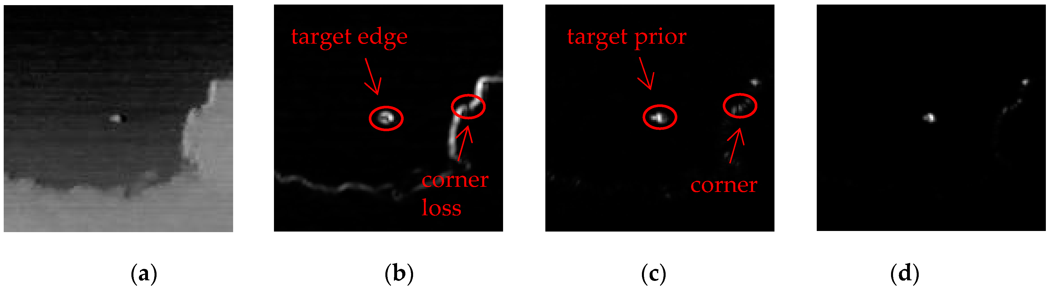
3.2. Local Prior Analysis

The grayscale-based measures that are used in most filtering methods are merely focusing on how to extract local prior such as local contrast [16,56,57], local entropy [58,59], and local difference [32,33,60]; nevertheless, this type of insufficient information is not enough to differentiate target and background. Conversely, optimizing methods with nonlocal property involved are more robust to complex scenes, but still suffer from background residuals in target components mainly because of the salient edges. Its intrinsic reason is because that the sparsity of the salient edges is similar to that of the targets. In fact, the stubborn edges can be easily identified by local prior, which means that the defects of optimizing methods can be alleviated via adding extra local prior. For this reason, the RIPT model employs structure tensor [61] to discriminate all of the image boundaries, since these boundaries tend to contaminate the sparse target matrix. The two highest eigenvalues λ 1 and λ 2 ( λ 1 λ 2 ) are applied to depict the local geometry structure. As the value of λ 1 λ 2 highlights image boundaries clearly, the local structure weight patch-tensor used in the RIPT model is defined as:
W LS = exp ( h ( 1 2 ) d min d max d min )
where 1 and 2 are the corresponding patch-tensors of two obtained eigenvalue matrices, h is a weight-stretching parameter, d max and d min are the maximum and minimum of 1 2 , respectively.
As analyzed in Section 1, the operator λ 1 λ 2 that is utilized to calculate W LS is completely poor at determining whether the edge components belong to the target or background. When serving as the local structure weight, such ambiguity causes the distortion of target shape, due to the similar weights between the background edge and the target edge. This situation becomes even worse with the increasing of h , as shown in Figure 5. We know that when locating at the corner region, λ 1 λ 2 0 ; when locating at the edge region, λ 1 λ 2 0 ; when locating at the flat region, λ 1 λ 2 0 . Hence, structure tensor tends to give lower values at corners even if some of them are part of the edges sometimes. As pointed out in [62], when the weight stretching parameter h decreases, the difference would be more significant, causing an increase in the false alarm rate. In summary, on one hand, to preserve the target and prevent it from being completely lost, a smaller h is needed; in contrast, to avoid the interference of residuals, a larger h is needed. This is contradictory and finding an appropriate value of h is difficult because the size of small target varies within a somewhat large range. Another disadvantage is that RIPT merely considers the background-edge-related prior while ignoring the target-related prior since both of them can cause false alarms.
Due to the objective existence of the target edge, it is hard to utilize operator λ 1 λ 2 to only obtain the background prior. To alleviate the issue of target over-shrinking and corner disappearance, a new local structure descriptor related to the target prior without an additional stretching parameter was exploited. In [63], a “corner strength” function was computed to find the interest points:
w cs ( x , y ) = det ( S T ( x , y ) ) tr ( S T ( x , y ) )    = λ 1 λ 2 λ 1 + λ 2
where ( x , y ) represents the pixel location, S T ( ) denotes the structure tensor, S T ( x , y ) is a matrix, d e t ( ) and t r ( ) are the determinant and trace of matrix respectively, and w c s ( x , y ) is the half of the harmonic mean of the eigenvalues ( λ 1 , λ 2 ) . Figure 6 indicates the map of interest points of an infrared image (i.e., Figure 6c) compared with the local structure weight (i.e., Figure 6b), which demonstrates two underlying facts: (i) the target information is highlighted that fully complies with our expectation, and (ii) the corner regions that have been lost in the local structure weight map used in RIPT are identified. Furthermore, we replaced the subtraction operator as the maximum between two eigenvalues, namely:
w m ( x , y ) = max ( λ 1 , λ 2 )
It should be noted that the same problems also exist in the maximum operator but not so badly.
Thus, as shown in Figure 6d, the final version of prior weight map W p is
W p ( x , y ) = w cs ( x , y ) w m ( x , y ) = max ( λ 1 , λ 2 ) λ 1 λ 2 λ 1 + λ 2
Then, the patch-tensor of the prior weight map with normalization is defined as:
W p = W p w min w max w min
where w max and w min denote the maximum and minimum of W p , respectively.

3.3. IPT Model Based on PSTNN

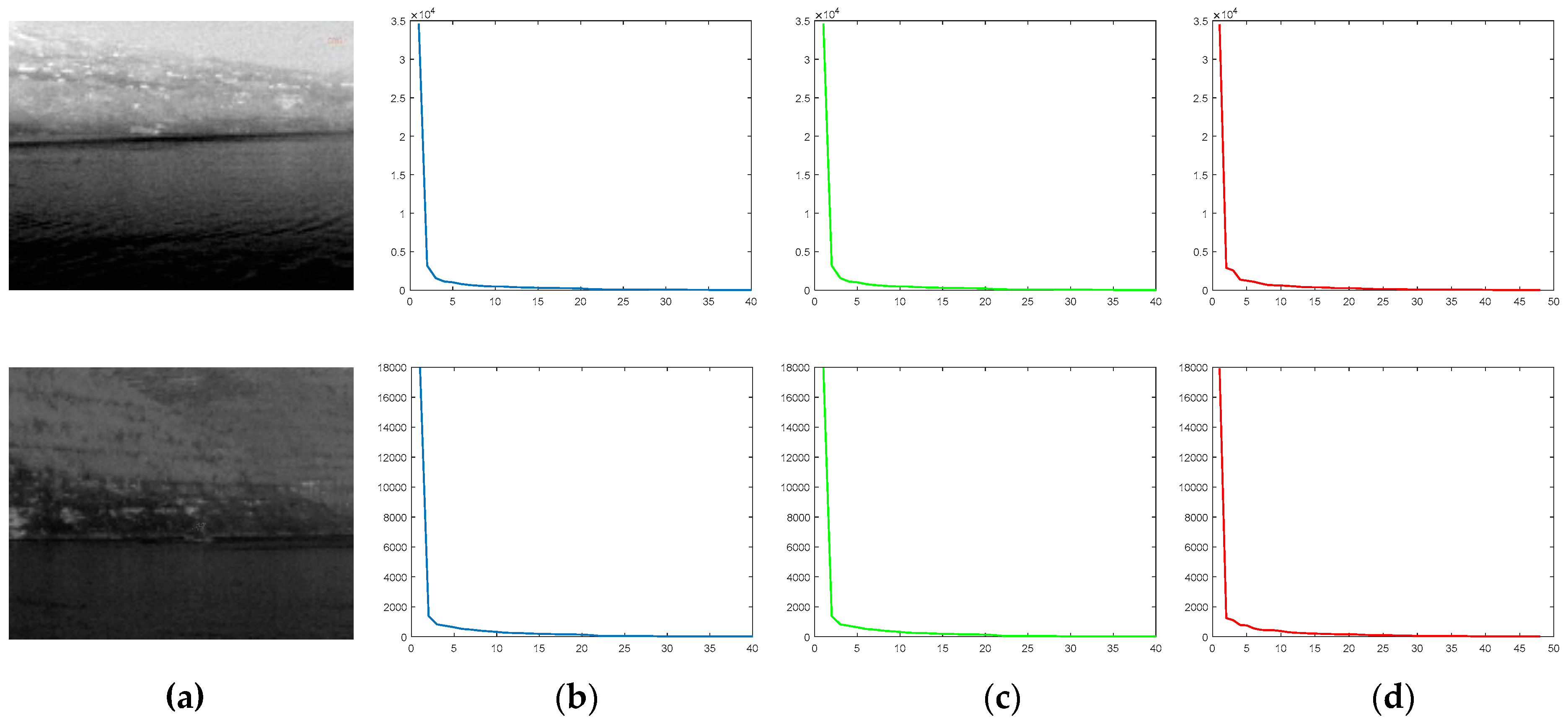
3.3.1. The Surrogate of Tensor Rank

Considering that the background changes slowly because of the high correlations among local and nonlocal patches, low rank is an intrinsic property of the infrared background. The straightforward measurement to access the low-rank characteristic of a tensor is the tensor rank. However, there is no direct way to extend the low-rankness from the matrices to tensors. More specially, due to the variety of tensor decomposition methods, the definition of tensor rank is not unique. The most popular definitions are CP rank [64] and Tucker rank [65]. Another difficulty lies in the tensor extension of RPCA (i.e., TRPCA) since the numerical algebra of tensors is fraught with hardness results [66]. How to choose a suitable tensor rank with a tight convex relaxation is of great importance.
In reweighted infrared patch-tensor (RIPT) model, the low-rank characteristic of the background patch-tensor is accessed via the sum of nuclear norms (SNN), which is based on the singleton model [43]. SNN, defined as i X ( i ) , is used as a convex surrogate of i rank ( X ( i ) ) . A rational fact behind the regularizer SNN is that the nuclear norm is the tightest convex envelope to matrix rank within the unit ball of the spectral norm. Besides, instead of calculating the complex tensor nuclear norm, SNN calculates the simpler matrix nuclear norm. Nevertheless, SNN is not a tight convex relaxation of i rank ( X ( i ) ) [45], which implies SNN has the limitation of obtaining suboptimal value. In other words, when served as a background constraint, SNN would produce false alarms.
Derived from t-SVD, the tensor nuclear norm (TNN) was proposed in [51] and successfully applied to image recovery which had shown its advancement compared to SNN. Generally, minimizing the TNN may cause some unavoidable biases [46]. Meanwhile, SNN and TNN treat each singular value equally which is irrational, since the larger singular values are generally associated with the image details; thus, they should be assigned smaller weights. To alleviate those phenomena, it’s appropriate to adopt a nonconvex relaxation with unequal weights. In [46], Jiang et al. extended the partial sum of singular values (PSSV) [50] to the tensor version and presented the partial sum of the tensor nuclear norm (PSTNN) to replace the TNN as the nonconvex approximation of tensor csor X n 1 × n 2 × n 3 is defined as
X PSTNN = i = 1 n 3 X ¯ ( i ) p = N
where p = N denotes the PSSV. Since the infrared backgrounds could vary from simple to complex, it’s better to employ an adaptively predicted rank constraint. On the contrary, considering that the small target only holds an extremely small part of the entire image, a simpler way to determine the parameter N is to set a fixed energy ratio without directly concentrating on the changeable backgrounds. To approximate the tensor rank with high accuracy, the PSTNN is a better candidate than SNN and TNN.

3.3.2. Model Construction

Likewise, we utilized the conventional way to relax the non-smooth and discrete l 0 norm. So the infrared small target detection model based on patch-tensors with the priors of target and background is as follows:
min , T     PSTNN + λ T W r e c 1                       s . t .     D = + T
where denotes the Hadamard product, W r e c is the tensor corresponding to elementwise reciprocals of the corresponding elements in W p , and       1 denotes the l 1 norm, which is the sum of the absolute values of all the elements.
In [67], Candès proposed a reweighted l 1 minimization to address the imbalance in which larger coefficients are penalized more heavily than smaller ones. Subsequently, the reweighted scheme achieved great success in many publications [68,69,70]. As indicated in Table 1, the computing time of optimizing methods is always a major concern. Therefore, to speed up the convergence rate, and reduce the time of the whole procedure, we adopted the reweighted scheme as well. The sparsity weight is defined as follows:
W s w k + 1 = c | T k | + ε
where c is a nonnegative constant, ε > 0 is a small number to avoid division by zero, and k+1 denotes the (k+1)-th iteration. In some cases, c is fixed to 1 [42,62]. We combined the two weights to get a simplified form
W = W s w W r e c
Then, Equation (19) is rewritten as follows:
min , T     PSTNN + λ T W 1                       s . t .     D = + T
In addition, as the same as analyzed in [42], we observed that the number of nonzero entries in target patch-tensor stops changing after a few iterations, which is just a little proportion of the entire procedure if the stop condition is when the relative error is smaller (i.e., + T D F 2 / D F 2 ) than a given threshold. Hence, to better utilize this observation and alleviate the imbalance between computing time and performance, the algorithm stops the iterations once the number of nonzero entries ceases to decrease or the relative error is smaller than the given threshold.

3.3.3. Solution of the Proposed Model

The alternating direction method of multipliers (ADMM) [49] has a fast convergence rate and high accuracy. In this section, an ADMM-based solver is devised to solve Equation (22). The augmented Langrangian function of Equation (22) is defined as
L μ ( , T , W , Y ) = PSTNN + λ T W 1 + Y , + T D + μ 2 + T D F 2
where Y is the Lagrange multiplier, denotes the inner product of two tensors,       F is the Frobenius norm, and μ > 0 is a penalty factor.
Then, the problem argmin , T , W , Y L μ ( , T , W , Y ) in Equation (23) can be separated as several subproblems, and in the (k+1)-th step, T and are updated as:
T k + 1 = argmin T λ T W k 1 + μ k 2 k + T D + Y k μ k F 2
k + 1 = argmin PSTNN + μ k 2 + T k + 1 D + Y k μ k F 2
The subproblem (24) can be solved easily via Theorem 2.3:
T k + 1 = S λ W k μ k ( D k Y k μ k )
The subproblem (25) is calculated by Theorem 2.2 utilizing Algorithm 1 in the Fourier domain, which is described in Algorithm 2 (please see Ref. [46] for details).
Y and μ update in the standard way:
Y k + 1 = Y k + μ k ( D k + 1 T k + 1 )
μ k + 1 = ρ μ k
where ρ > 1 . Finally, the whole process is described in Algorithm 3.
Algorithm 2 Solve Equation (25) using PSVT
Input: A k = D T k + 1 Y k μ k n 1 × n 2 × n 3 , λ , μ k
1. Compute A ¯ k = f f t ( A k , [ ] , 3 )
2. Compute each frontal slice of ¯ k + 1 by
for i = 1 , , ( n 3 + 1 ) / 2 do
   ( ¯ k + 1 ) ( i ) = P N , λ / μ k ( ( A ¯ k ) ( i ) ) (Operator P ( ) is defined in Equation (7));
end for
for i = ( n 3 + 1 ) / 2 + 1 , , n 3 do
   ( ¯ k + 1 ) ( i ) = c o n j ( ( ¯ k + 1 ) ( n 3 i + 2 ) ) ;
end for
3. Compute k + 1 = i f f t ( ¯ k + 1 , [ ] , 3 )
Algorithm 3 ADMM solver to the proposed model
Input: D , W p , λ , μ 0 , ε , N
Initialization: 0 = T 0 = Y 0 = 0 , W s w = 1 , W 0 = W r e c W s w , μ 0 = 3 × 10 3 , ρ = 1.1 , c = 1, k = 0
while not converge do
 1. Fix the others and update T k + 1 by Equation (26);
 2. Fix the others and update k + 1 by Algorithm 2;
 3. Fix the others and update Y k + 1 by Equation (27);
 4. Fix the others and update W k + 1 by
   W s w k + 1 = c | T k | + ε ;
   W k + 1 = W r e c W s w k + 1 ;
 5. Update μ by Equation (28);
 6. Check the convergence conditions
   k + 1 + T k + 1 D F 2 D F 2 < ε or T k + 1 0 = T k 0 ;
 7. Update k: k = k+1;
end while
3. Output: k , T k

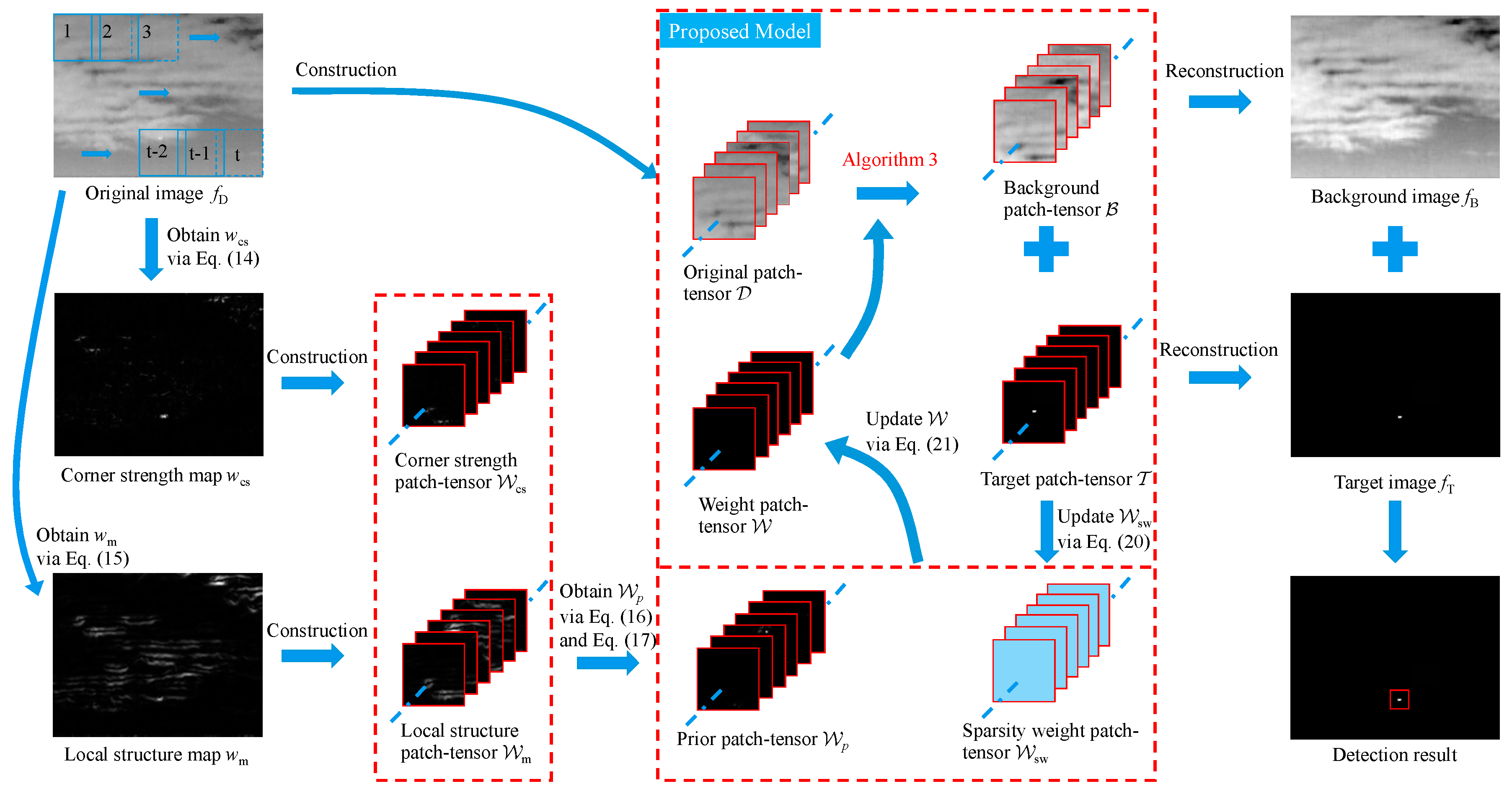
3.4. The Whole Procedure of the Proposed Method

Figure 7 shows the whole procedure of the infrared small target detection method based on the proposed model, which can be described as follows:
(1).
Local prior extraction. Given an infrared image, by calculating Equation (16), the prior weight map W p related to the target and background information is obtained.
(2).
Patch-tensor construction. By sliding a window of size k × k from top left to bottom right to transform the original infrared image f D m × n and the prior weight map W p m × n into the original patch-tensor D k × k × t and the prior weight patch-tensor W p k × k × t respectively, where t is the number of window sliding.
(3).
Target-background separation. The input patch-tensor D is decomposed into a low-rank patch-tensor k × k × t and a sparse patch-tensor T k × k × t via Algorithm 3.
(4).
Image reconstruction and target detection. The target image f B m × n and background image f T m × n are reconstructed from the low-rank patch-tensor k × k × t and sparse patch-tensor T k × k × t , and the process of reconstruction is contrary to that of construction. Meanwhile, a one-dimensional median filter is exploited to determine the value of the position overlapped by several patches. Once the reconstruction is done, small targets are detected easily via adaptive threshold segmentation as in [20].

4. Experiment and Results

In this section, extensive experiments are conducted to verify the feasibility of the proposed model from different aspects including robustness against various scenes, robustness to noise, the ability of background suppression and target enhancement, target detection ability, and the computation time of the algorithm. To fully access the superiority of the proposed algorithm, nine state-of-the-art approaches are included for comparison.

4.1. Experimental Setup and Description

The diversity of scenes is one of the biggest challenges for detecting small targets embedded in infrared images. In order to validate the robustness of our approach to scenes, 24 infrared images with different varied scenes from uniform backgrounds with extremely dim targets to complex scenes with salient interferences and clutters were tested, which are displayed in Figure 8. All of the targets are marked with red (or green) square boxes. Moreover, for the sake of better observation and comparison, we had enlarged the target areas and then placed most of them in the lower left (right) corner of the image. Following this, six typical scenes were chosen from the 24 tested images to evaluate the performance of our method in the case of noise with different levels. Note that the added noise obeys the Gaussian distribution. Next, four sequences (Figure 8a–d) were used to quantify the detection ability of the proposed model. Finally, the algorithm complexity and computation time for different sizes are given. Nine methods including the Top-hat filter [12], Laplacian of Gaussian (LoG) filter [29], multiscale patch-based contrast measure (MPCM) [31], relative local contrast measure (RLCM) [19], infrared patch-image model (IPI) [20], nonnegative infrared patch-image model based on partial sum minimization of singular values (NIPPS) [21], reweighted IPI (ReWIPI) [38], nonconvex rank approximation minimization (NRAM) [39], and reweighted infrared patch-tensor model (RIPT) [42] were employed as the baselines. The same experiments were carried out with these baselines for all-round comparison. Given space limitations, only part of the experimental results are shown in this paper; the full extent can be found in the Appendix A and Appendix B. Table 3 summarizes the parameter settings of all the methods used in this paper. All of the optimizing methods, i.e., IPI, NIPPS, ReWIPI, NRAM, RIPT and the proposed method were solved via ADMM. In addition, all of the experiments were implemented with Matlab R2018a in Windows 7 based on Intel Celeron 2.90 GHz CPU with 4G of RAM.

4.2. Evaluation Metrics

In this subsection, for a comprehensive comparison with the aforementioned state-of-the-art approaches, several typical metrics, including the signal-to-clutter ratio gain (SCRG), the background suppression factor (BSF), and the receive operating characteristic (ROC) curve with the area under curve (AUC) were used, where the ROC curve shows the tradeoff between the detection probability P d and false-alarm probability F a . These metrics would reveal the ability of one method in target enhancement, background suppression, and target detection. The most widely used criterion SCRG is defined as
SCRG = SCR out SCR in
where subscripts out and in represent the original image and the obtained target image respectively, and SCR is a measurement of the difficulty of detecting a small target in an infrared image, whose definition is
SCR = | μ t μ b | σ b
where μ t is the average grayscale of the target area, μ b and σ b are the average pixel value and standard deviation of the surrounding local neighborhood region, respectively.
Another evaluation indicator is BSF, showing the background suppression quality of detection algorithms, which is defined as
BSF = σ i n σ o u t
where σ i n and σ o u t stand for the standard deviation values before and after suppression in the local region. SCRG and BSF are calculated in the neighborhood region around the target, and Figure 9 shows the local region that is used in the experiment. Assuming that the target size is a × b , then the local region size is ( a + 2 d ) × ( b + 2 d ) ; we set d = 20 in this paper.
In addition to the above two evaluation indicators, the detection probability P d and false-alarm probability F a is a pair of key metrics, which are defined as follows:
P d = number    of    true    detections number    of    actual    targets
F a = number    of    false    detections number    of    images
The ROC curve is drawn according to P d and F a values, where F a is abscissa and P d is ordinate. The AUC is the area enclosed by the ROC curve and the coordinate axis. Except for ROC, for all the other metrics, the larger their value, the better the performance of the method.

4.3. Parameter Analysis

For the proposed model, there are several important parameters such as the patch size, the sliding step, the penalty factor μ , and the tradeoff constant λ that usually affect the robustness for different scenes. Hence, to obtain a better performance with real datasets, it is wise to choose proper parameters via experiments. The ROC curves on four real infrared sequences for different model parameters are given in Figure 10. Here, one point needs to be noted is that the performances obtained by tuning one of the parameters with the others fixed may not be globally optimal.

4.3.1. Patch Size

Patch size plays a vital role in determining not only the detection performance, but also the computation complexity of the algorithm. We hope for a larger patch size to make sure that the target is sparse enough due to the uncertainty of the target size; however, some noise with sparsity properties such as salient edges would also have a higher probability of being identified as target components, which degrades the separation results. On the other hand, a smaller patch size would lead to a smaller computational complexity in each inner loop with singular value decomposition (SVD), but the sparseness of the target is no longer so obvious. To figure out the influence of the patch size on Sequences 1–4, we varied the patch size from 20 to 60 with 10 intervals and the corresponding ROC curves are illustrated in the first row of Figure 10. By analyzing the ROC curves, we can conclude that the best performance is achieved when the patch size is set to 40 for all of the sequences. The worst performance is reached when the patch size is equal to 60 in most cases. This is because a too-large patch size would regard the salient non-target noise as the “true” target, also resulting in incorrect recovery, especially when the target is not so prominent. The performance of 20 depends on the target size as the target in Sequence 1 is very dim and small while it breaks down when dealing with larger targets in Sequences 3–4, which results from the lack of target sparsity. Another underlying fact is that our proposed model is a little sensitive to the patch size particularly when facing extreme complex scenes such as those in Sequence 1, the target of which is almost submerged. Therefore, we chose 40 as the best patch size utilized in the following experiments.

4.3.2. Sliding Step

Similar to the patch size, the sliding step has a direct impact on the construction of patch-tensor, which indirectly influences the computation time and detection performance simultaneously as well. The sliding step determines how many frontal slices we can obtain to compose the desired patch-tensor. Different from other similar models, we prefer a larger sliding step which results from the following reasons. (i) A smaller sliding step implies that there would be more frontal slices containing the target, leading to an insufficient sparseness of the target, and (ii) More frontal slices means an increased computation time of t-SVD in Algorithm 1, because more inner loops are needed to calculate the matrix SVD of each frontal slice. To investigate its actual influence, we show the effects of the sliding step in the second row of Figure 10 via varying it from 10 to 40 (based on the best value of the patch size) with five intervals. It can be observed that as the sliding step increases, the model works better. Ten is a commonly used value; however, it performs the worst. Furthermore, even if the sliding step changes slightly, this change has a great impact on the results, which means that the proposed model is very sensitive to this parameter. Hence, the best choice for the sliding step is 40.

4.3.3. Penalty Factor μ

μ controls the tradeoff between the low-rank background and sparse target, namely the PVST operator and soft-thresholding operator; thus, one has to choose μ carefully in order to ensure both optimality and a fast convergence rate. With a smaller μ , more details would be preserved in the background patch-tensor; nevertheless, the target may suffer from over-shrinking because its details are remained by the background. In contrast, a larger μ could protect the target, but might leave more non-target components in the target patch-tensor. To choose an appropriate value of μ for obtaining better detection ability and a lower false alarm ratio, we investigated the influence of penalty factor on Sequences 1-4 by changing μ from 1 × 10 3 to 9 × 10 3 with an interval of 0.002, as illustrated in the third row of Figure 10. From the results we can arrival at a conclusion that μ cannot be too large or too small, especially when μ = 1 × 10 3 ; the target is totally lost in most cases. Therefore, 3 × 10 3 was used to get a better balance between the background patch-tensor and the target patch-tensor.

4.3.4. Compromising Parameter λ

λ is a compromising parameter that controls the tradeoff between the target patch-tensor and the background patch-tensor. Hence, it is of great importance to fine tuning λ . With reference to [48], we set λ as L / max ( n 1 , n 2 ) n 3 and vary L from 0.2 to 1.4 instead of varying λ directly. We show the influence of λ on Sequences 1-4 in the fourth row of Figure 10. From the illustration, we can easily observe that when L = 1.2 and L = 1.4 , the performance of the proposed method is always worst. That is because as λ increases, the target patch-tensor would be suppressed to keep the whole objective function at a minimum, and vice versa. In other words, on one hand, a larger λ leads to a cleaner target image, but the target would be over-shrunk; on the other hand, a smaller λ can keep the target complete, but background residuals would be kept too. How to find the balance is a serious task. The experimental results shows that the performance is relative well when L = 0.6 . Then, λ = 0.6 / max ( n 1 , n 2 ) n 3 was used at the end.

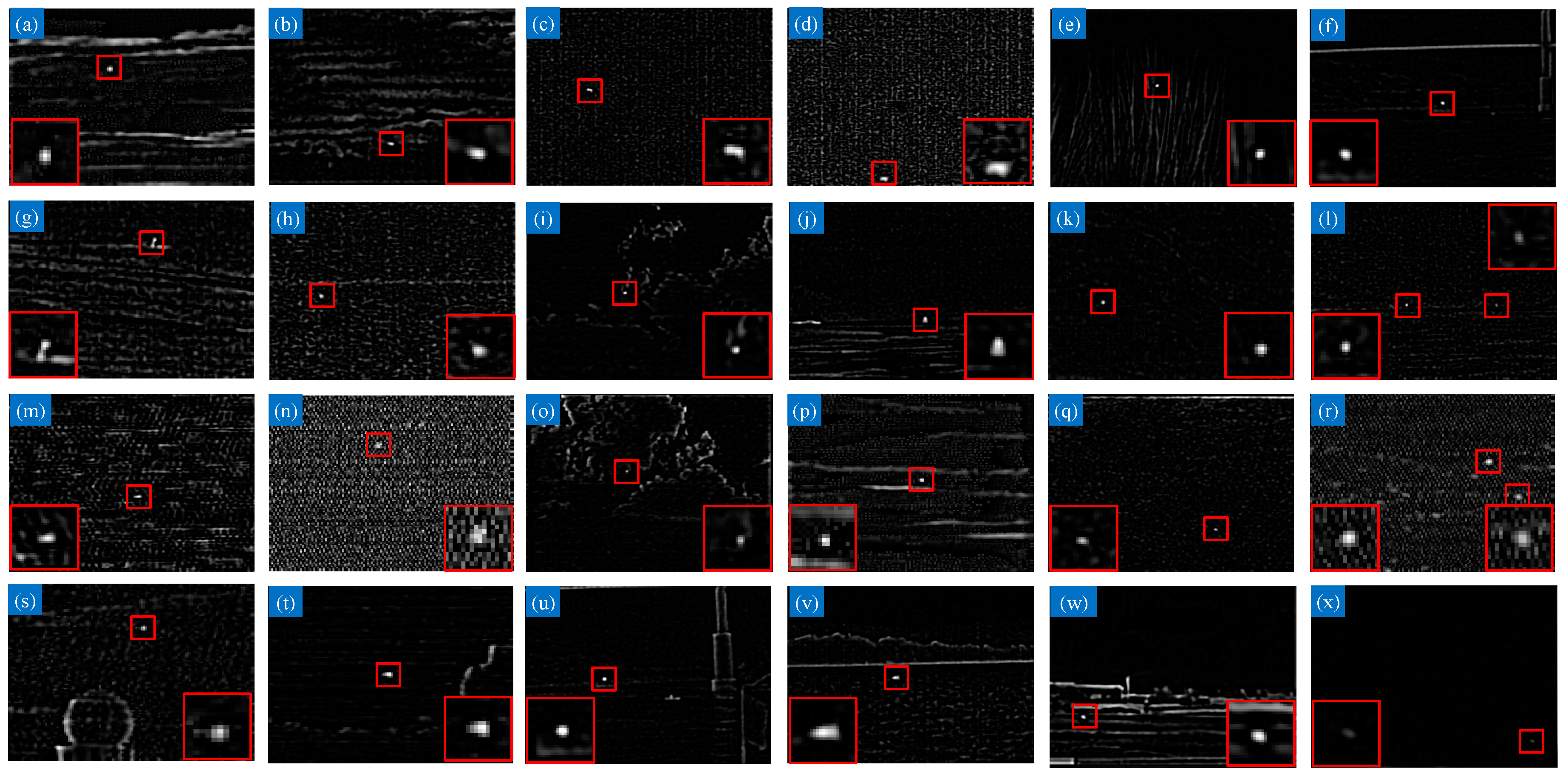
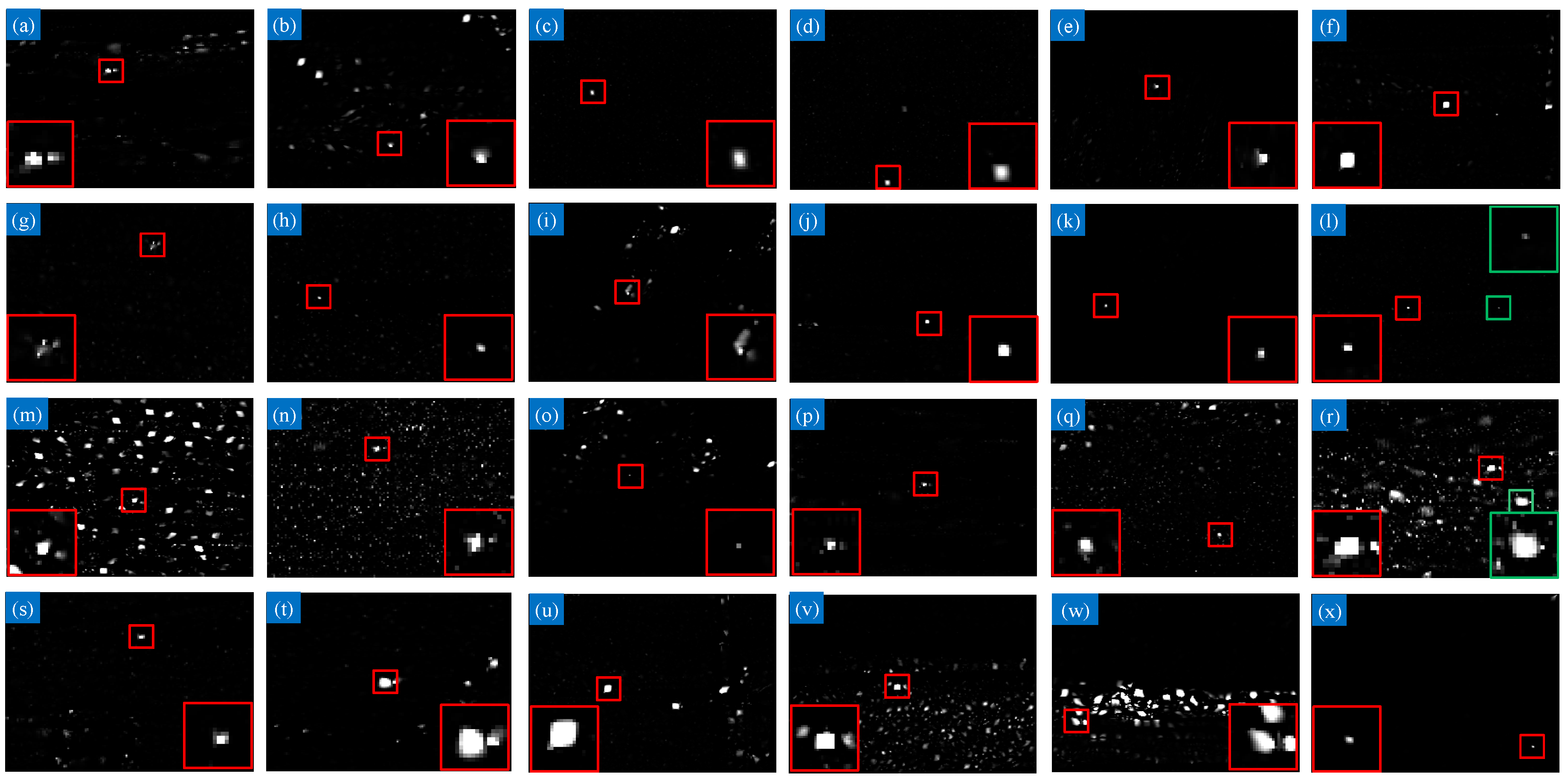
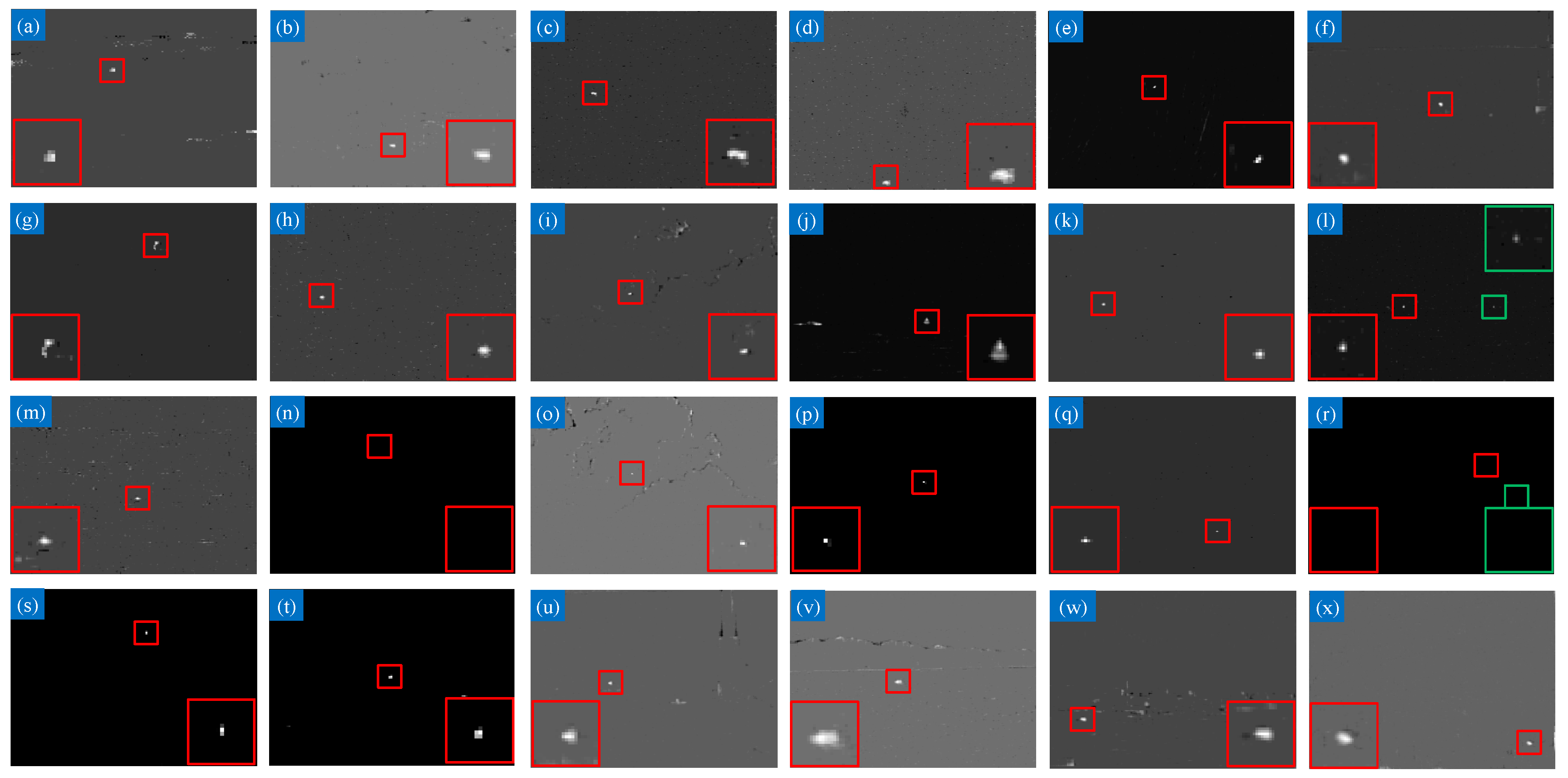
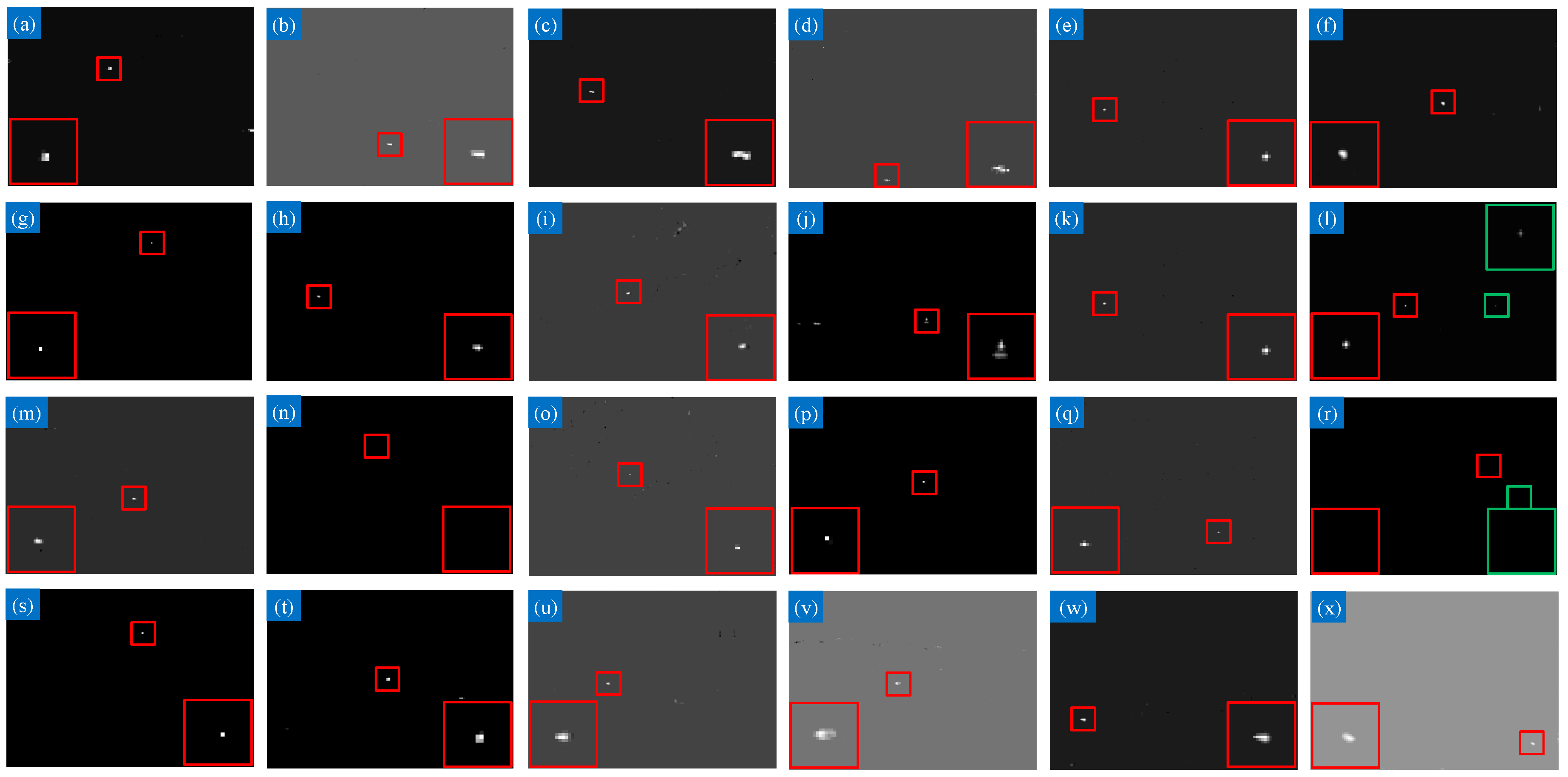
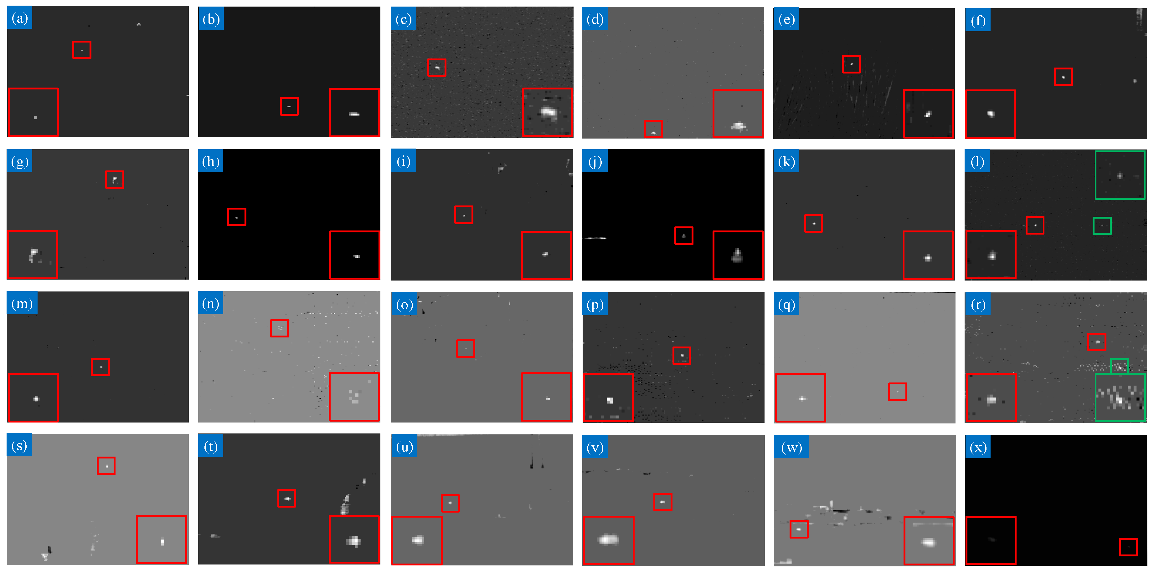
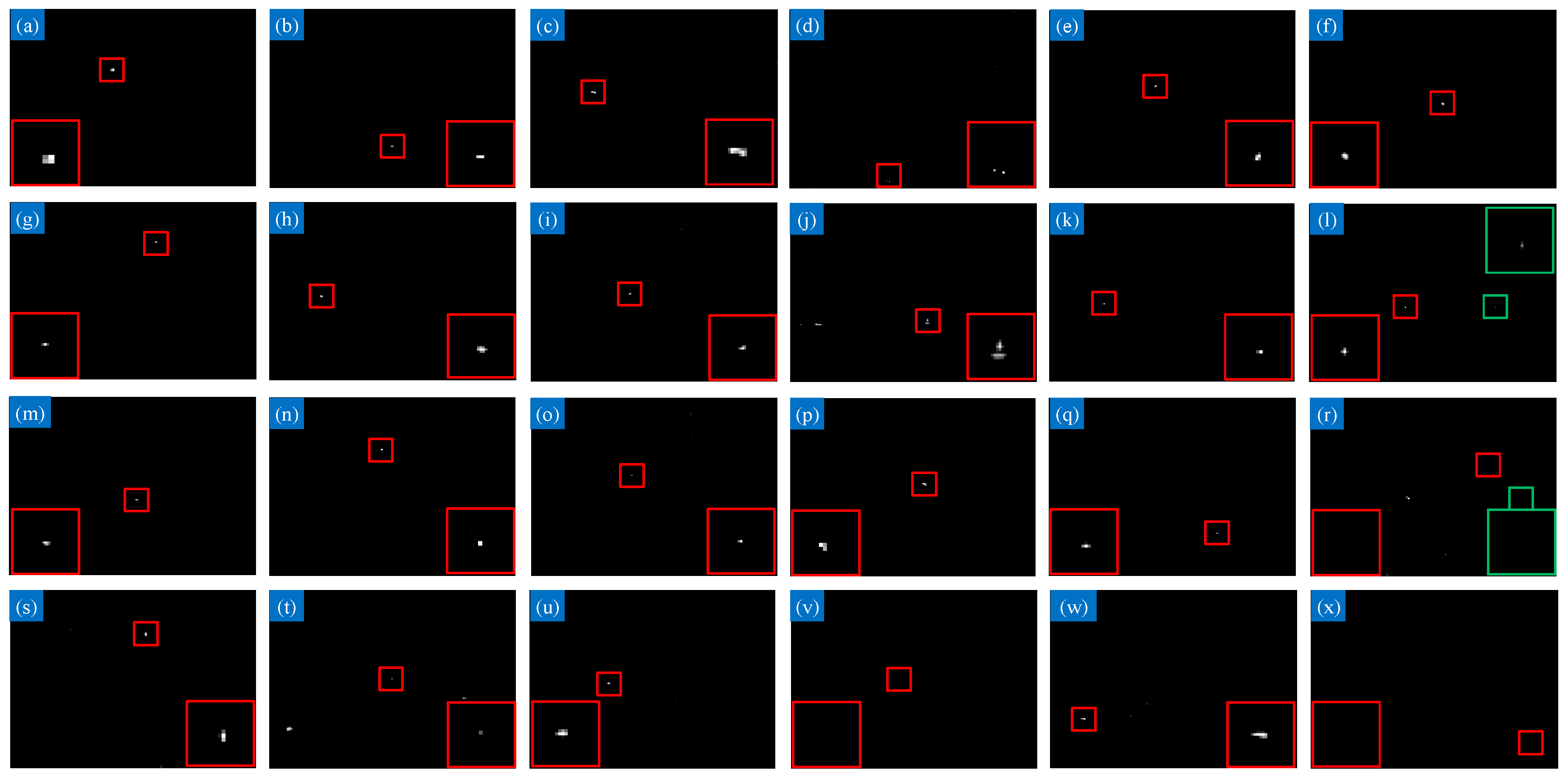
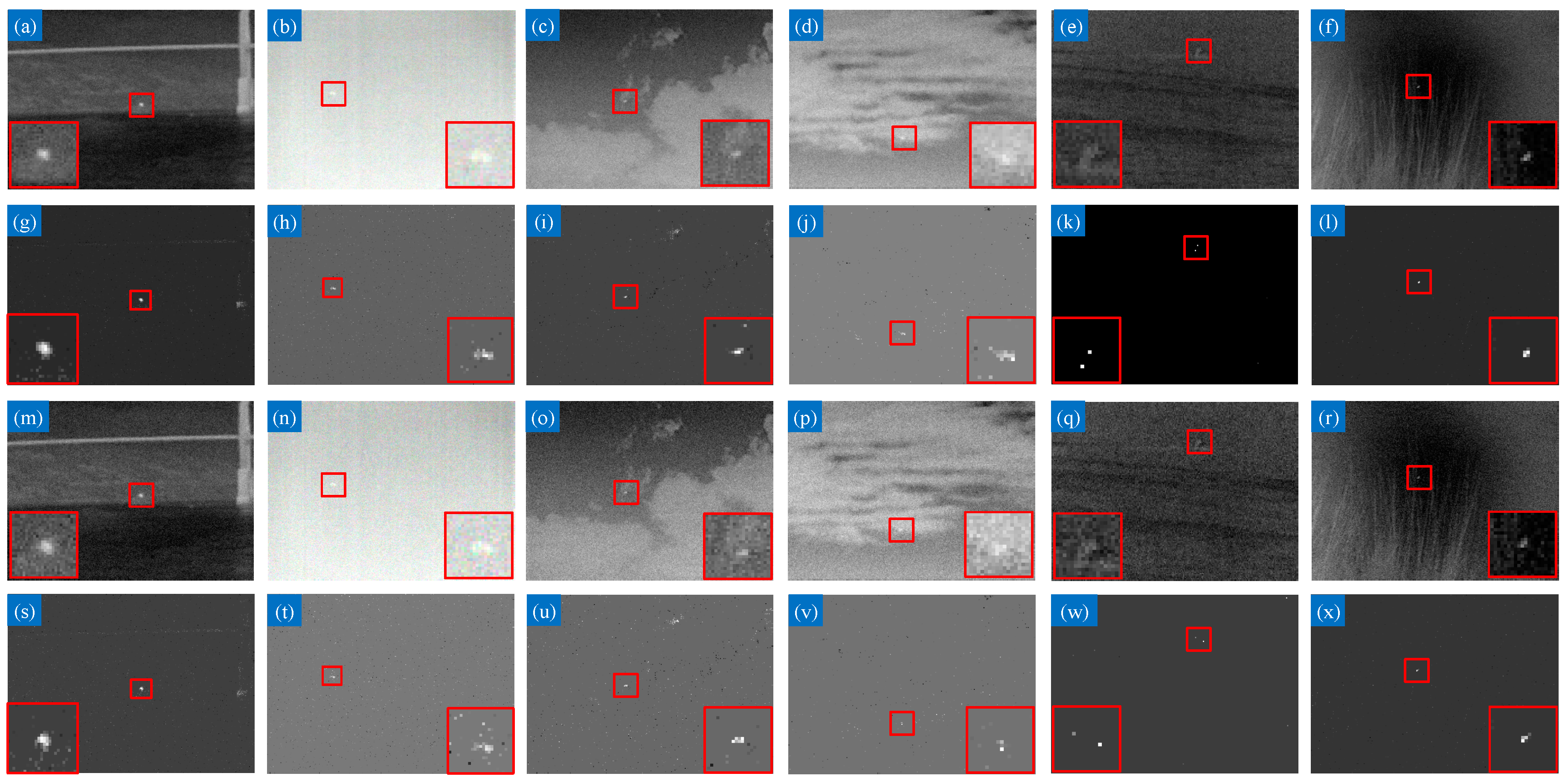
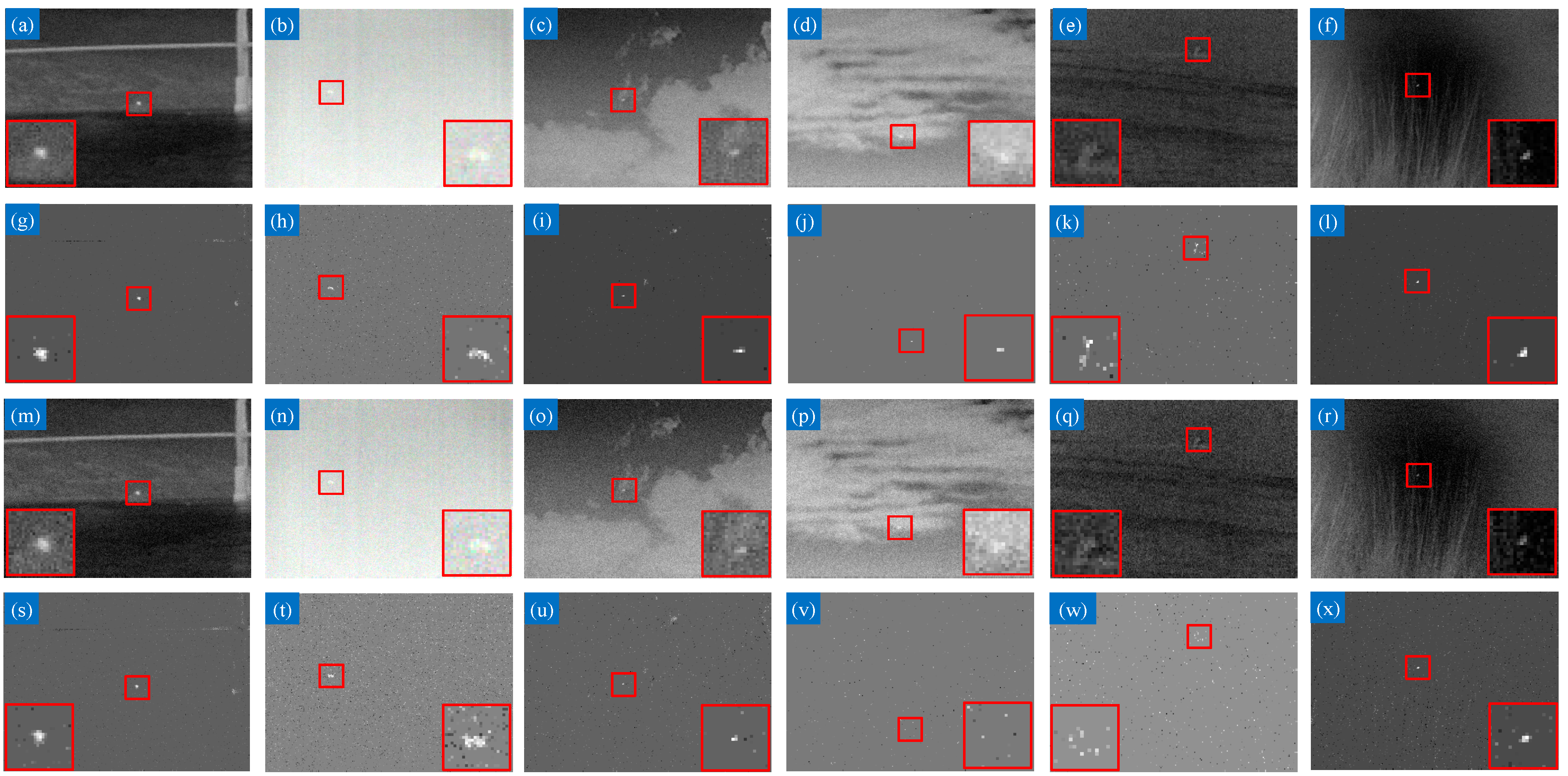
4.4. Qualitative Evaluation

In this subsection, the proposed method is compared with nine state-of-the-art methods from qualitative aspects, i.e., robustness to different scenes and Gaussian noise, which reflects the ability of target enhancement and background suppression of each approach. Note that due to the large number of images, the results of all the methods except the proposed model and RIPT model are in the Appendix A and Appendix B.

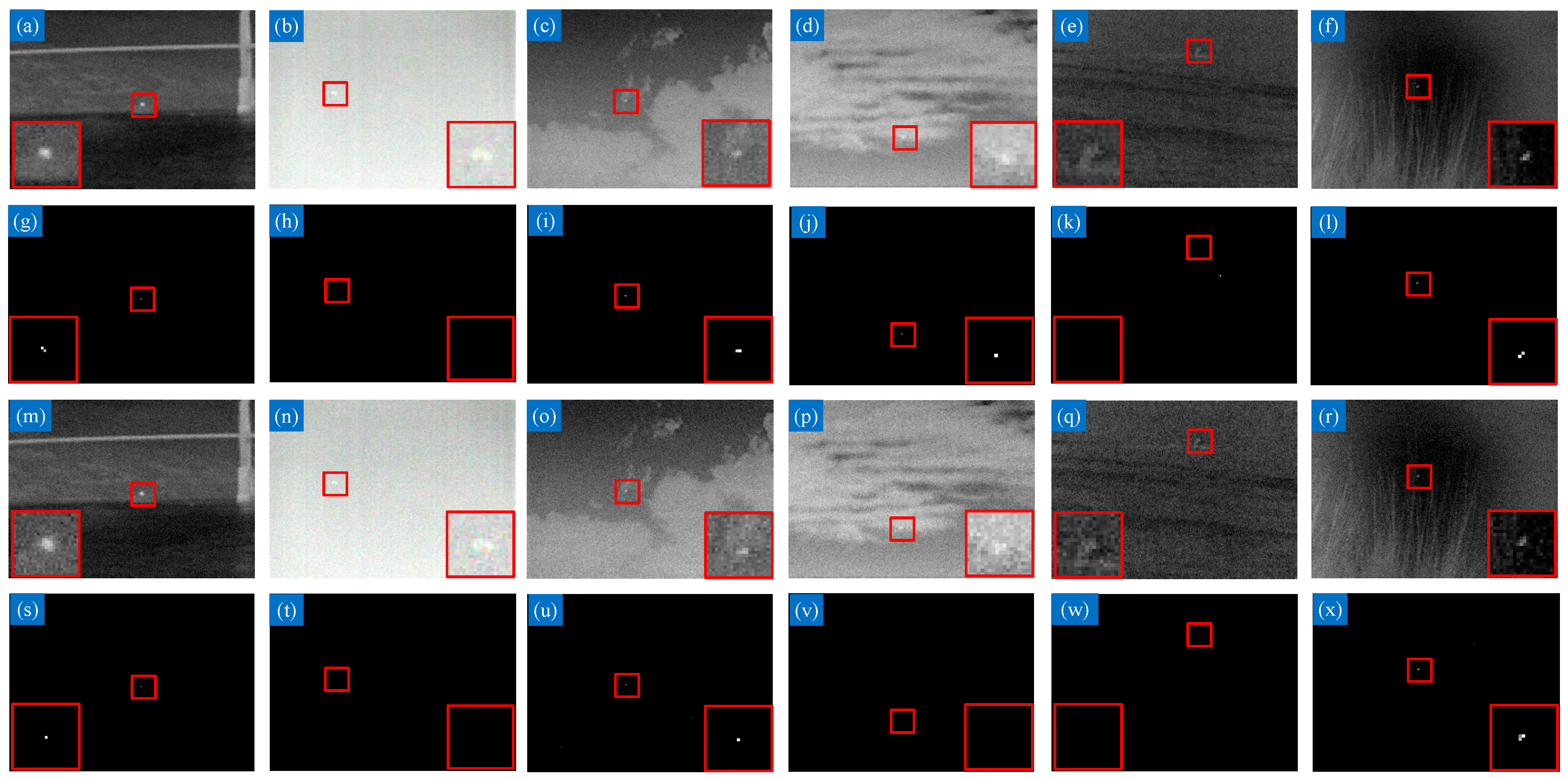
4.4.1. Robustness to Different Scenes

One major challenge of infrared small target detection lies in its variety, which has two-fold meanings. Firstly, infrared scenes are diverse, such as sky background with thick clouds such as those in Figure 8b, a sea background with buildings and moving ships such as those in Figure 8f, a messy background with lots of salient interferences such as those in Figure 8w, etc. Secondly, the size of the small target is not fixed, but varies within a large range. For instance, as shown in Figure 8o, the target embedded in the cloud layer can be viewed as a point target, while the target in Figure 8t is much bigger than the aforementioned one. Therefore, a useful way to verify whether a detection method is good or not is to test its robustness against different scenes containing different target sizes. The separated target images obtained from the proposed model under 24 different scenes are displayed in Figure 11, from which we can observe that the backgrounds are totally wiped out, remaining merely the desired targets. Meanwhile, the shape of the targets has also been basically preserved.
Figure 12 indicates the results processed by the RIPT model; as analyzed in Section 3.2, it is easy to observe that the RIPT model is suitable for dealing with a spot-like target, but when it comes to a non-spot-like target, the issue of over-shrinking happens, which results from the local structure weight treating the target edge and background edge equally, as shown in Figure 12c,t,u. In addition, the suboptimality of SNN brings about remaining residuals (noise) in target images such as those in Figure 12a,n. One more point worth mentioning is that the RIPT model may suffer from totally losing the target when the background and target are both dim, such as in Figure 12d,h. The results of handling the remaining methods with various scenes are displayed in Figure A1, Figure A2, Figure A3, Figure A4, Figure A5, Figure A6, Figure A7 and Figure A8 in Appendix A, from which it is clear that they all lack robustness. Hence, compared with these baselines, it’s fair to say that the proposed method shows advancement in dealing with different scenes and targets simultaneously.

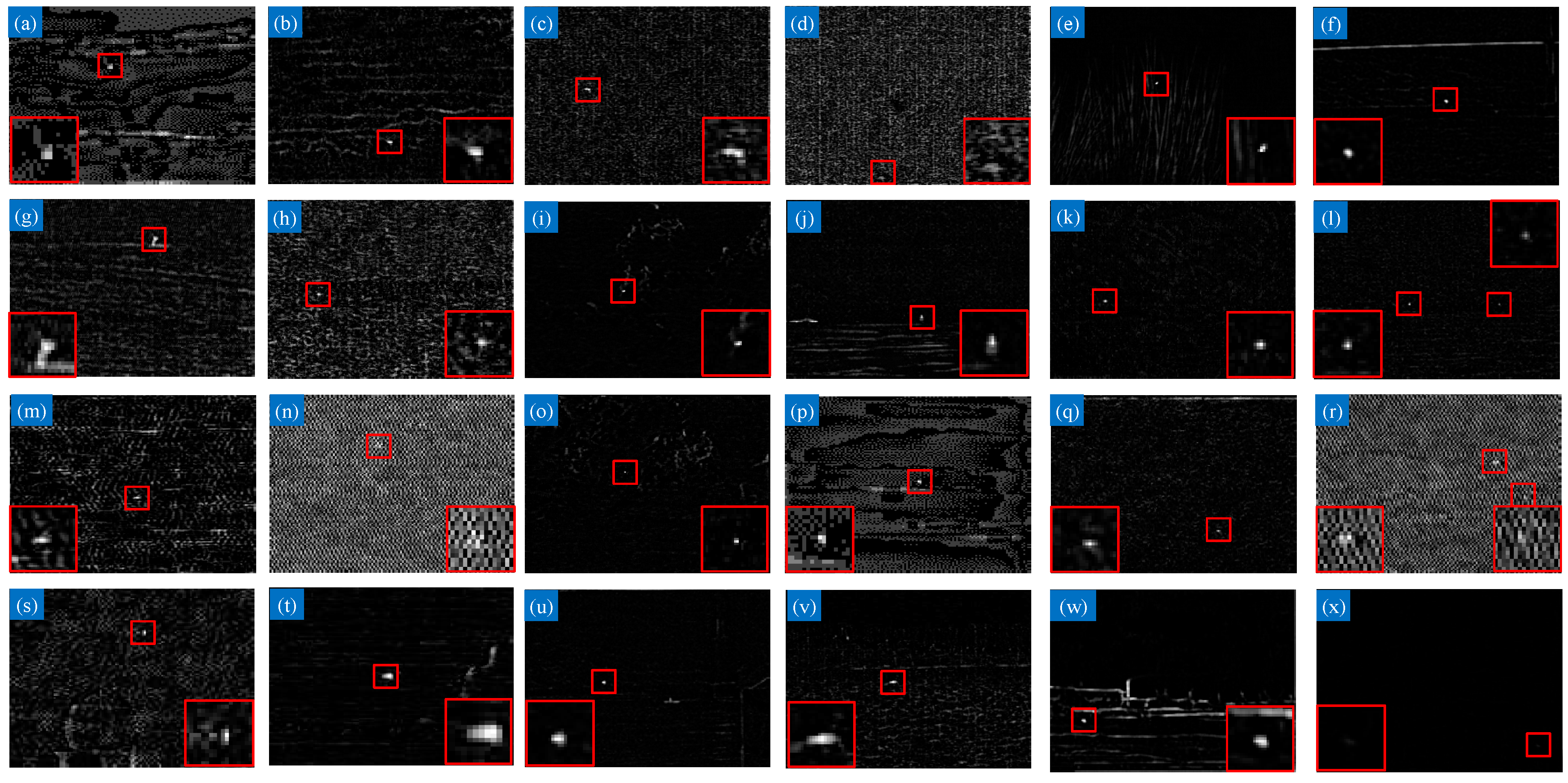
4.4.2. Robustness to Noise

In addition to various scenes, noise is also a key factor that affects the detection results. In Figure 13, we further evaluated the proposed model in terms of noise with different levels under six scenes selected from Figure 8. Gaussian noise with a mean of zero was imposed to the images in the first row and third row of Figure 13, respectively. When the standard deviation is 10, the proposed method performs relatively well regarding background suppression and target enhancement, as well as preserving the shape of the target. When the standard deviation increases to 20, the proposed method still accurately locates the targets and wipes out the backgrounds in Figure 13s,u,x. Unfortunately, in Figure 13t,v,w, the detected results deviate from the real targets regardless of shape or size. This is acceptable considering the noise is so dense that the target can hardly be detected. We can also conclude that as long as the target in the contaminative image is still relative salient such as in Figure 13a–f, the proposed method can work.
We show in Figure 14 the performance of the RIPT model dealing with different levels of noise. As can be seen from the figure, the target is more likely to be lost. Furthermore, although the target is still salient within a noise-containing background (Figure 14a,m for instance), the target recovered via RIPT is only spot-like, which demonstrates its weakness in handling slightly larger targets one more time. The results of the remaining optimizing methods facing noise are displayed in Figure A9, Figure A10, Figure A11 and Figure A12 in Appendix B. We can easily observe that they all have unsatisfactory performances, especially when the standard deviation is 20.

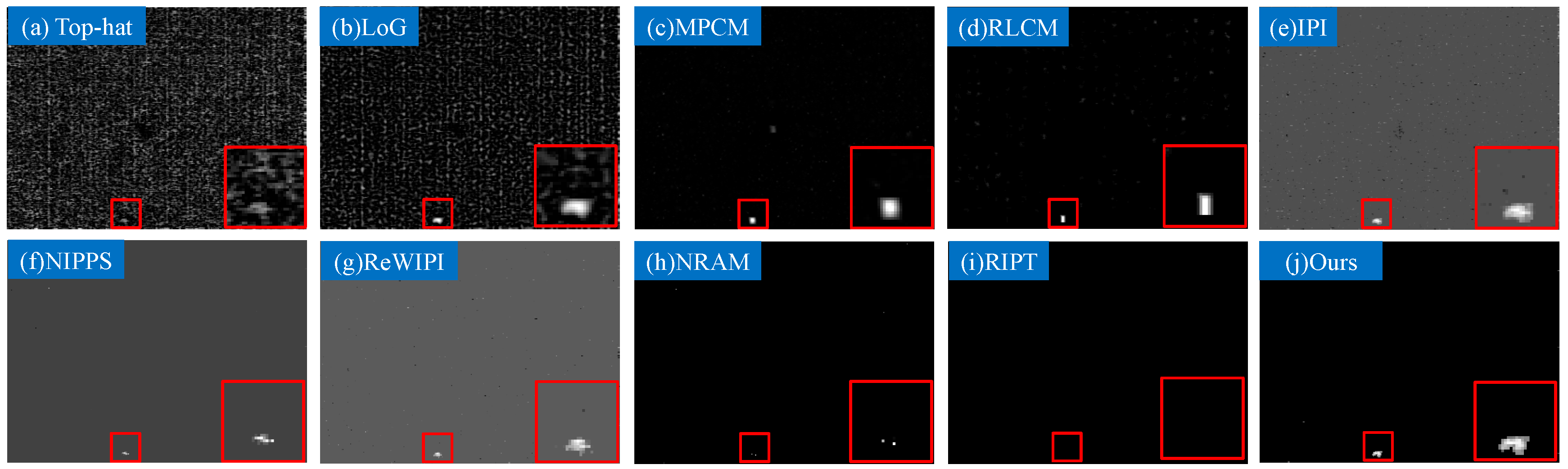
4.4.3. Visual Comparison with Baselines

To further visually compare the performance of all the competing methods, the results obtained by all the tested methods on Sequences 1–4 are displayed in Figure 15, Figure 16, Figure 17 and Figure 18, and the detailed descriptions of four sequences are shown in Table 4. Note that for the convenience of observation, the contrast of the results obtained by Top-hat, LoG and RLCM is adjusted. For conventional Top-hat transformation, it can highlight the target to a certain extent in Figure 15a, Figure 16a, Figure 17a and Figure 18a; however, it is extremely sensitive to noise and clutters, which would produce many false alarms. The intrinsic reason is mainly relevant to the usage of the fixed structural element without considering the surrounding neighborhood. Besides, the fixed structural element with a fixed shape is difficult to perfectly match all the targets. LoG, MPCM and RLCM are all HVS-based approaches but the performance of LoG is much worse than the latter two. We can obviously see that LoG is also vulnerable to edges and noise which results from the calculation of Gaussian scale space and its second derivative, making the target and edges both enhanced, especially in the case of complex background such as those in Figure 15b and Figure 16b. The main difference between MPCM and RLCM is the definition of local contrast measure, leading to distinguishing a detection ability. For MPCM, its local contrast measure is defined based on the difference between the current patch and its adjacent background patches; while for RLCM, the local contrast is associated with the mean grayscale value of each cell. Their improvement is apparent when facing uniform scenes, and the RLCM is slightly better than the MPCM from Figure 17c and Figure 18d. Nevertheless, just as the results in Figure 15 and Figure 16, the phenomenon of enhancing non-target pixels still exists, which is caused by the inaccuracy of the local dissimilarity measure; in some cases, they are even brighter than the real target.
Generally speaking, the rest of the optimizing methods show superiority in both target enhancement and background suppression. From the figures, there’s no doubt that IPI suffers from residuals in the recovered target image, because the matrix nuclear norm treats all the singular values equally, which usually leads to suboptimal solutions. Via minimizing the partial sum of singular values, NIPPS achieves a better performance than IPI. However, as observed in Figure 15f and Figure 18f, either a complex scene including highlight interferences and intensive noise or a particularly dim scene is still a challenge for NIPPS. To overcome the deficiencies of initial IPI, the ReWIPI adopts weighted technology to restore the background and target simultaneously. We can see from the results that the ReWIPI lacks robustness to different scenarios although it does well in Figure 16g. NRAM provides a tighter surrogate of rank with nonconvex rank approximation involved, which implies that the separated background image would be more accurate so that the problem of residuals could be solved. NRAM reaches the desired results except for the last sequence, from which the target is almost disappeared.
Unlike these matrix-level methods, RIPT directly stacks the patches into a tensor named patch-tensor without vectorizing each patch into a vector, which successfully converts a low-rank matrix recovery problem into a tensor recovery problem. As an extension of the IPI model, RIPT accurately captures the low-rank property of the matrix that is obtained by unfolding the patch-tensor along each mode, and thus achieving better detection performance. However, there are two issues for which the RIPT model has not been resolved: namely, salient noise such as that in Figure 15i, and target distortion with the possibility of completely loss such as that in Figure 18i. The proposed method shows superior performance not only in the preservation of the target but also in the suppression of backgroundcompared with the above baselines, especially in Figure 15 and Figure 18. Basically, all the methods are not performing well, except for ours. Furthermore, the computation time of the proposed method is less than that of the similar optimizing methods, which will be discussed later.

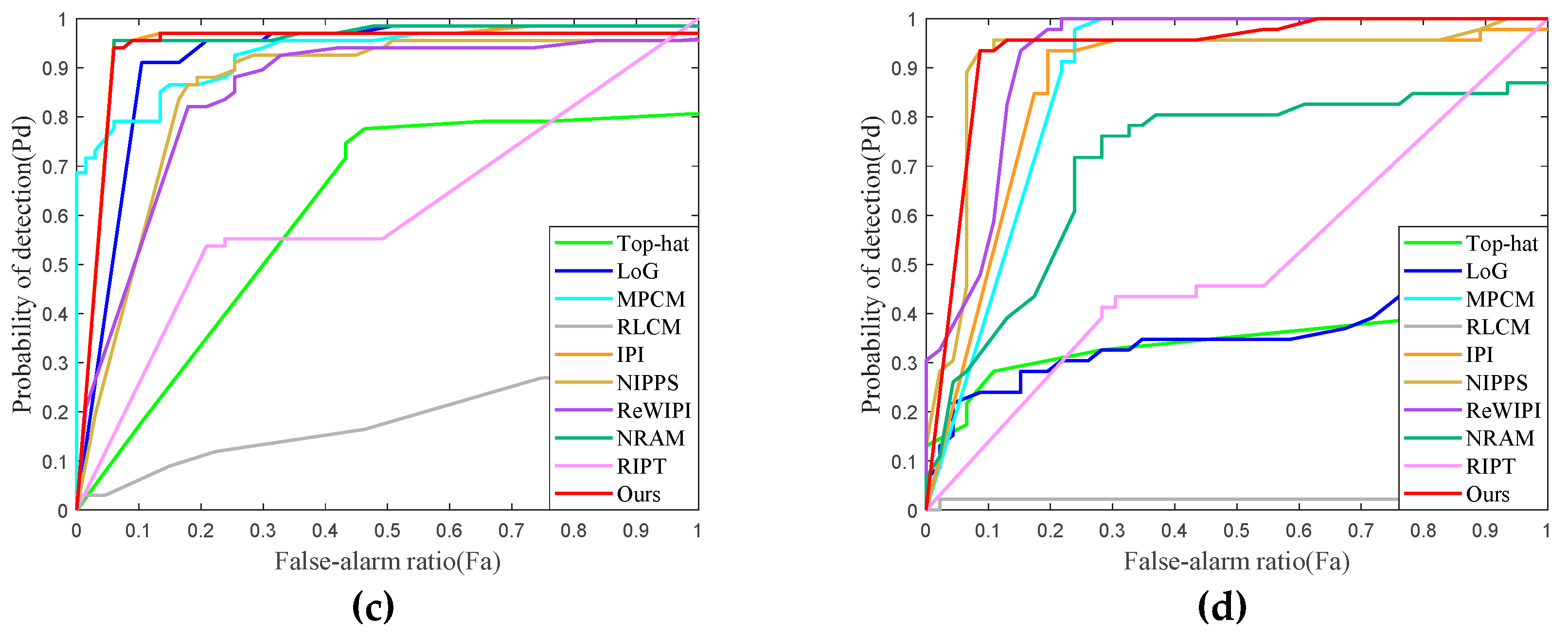
4.5. Quantitative Evaluation

Apart from visually validating the robustness of our method through single-frame images with different backgrounds and different noise levels, in this subsection, the detection performance of our model and other baselines was further measured via quantitative evaluation indicators including the signal-to-clutter ratio gain (SCRG), background suppression factor (BSF), and ROC curves on four real sequences. Table 5 lists the experimental results for all 10 tested approaches for Sequences 1–4. It should note that inf (i.e., infinity) represents the background is completely wiped out in the local region. Since NRAM and RIPT are not able to detect the target in Sequence 4 in some cases, when calculating SCRG and BSF for the last sequence, we don’t take these two methods into account. It can be clearly seen that the proposed method achieves the highest values in terms of SCRG and BSF in all of the datasets, showing great advantages in background suppression and target enhancement. On the other hand, RIPT gets the second highest scores sometimes in terms of the two metrics, which suggests that the tensor model can indeed seek more spatial information to improve the robustness. Filtering methods get very low scores in comparison with optimizing methods, resulting from the simple assumption based on background homogeneity or target saliency.
To further demonstrate the advantage of the proposed method, ROC curves corresponding to the four sequences that reflect overall detection ability of one method are plotted in Figure 19, and the AUC values are also listed in Table 6. A higher AUC value means that an algorithm has better performance. The performance of RLCM fluctuates greatly; for Sequences 1 and 2, RLCM works very well, but fails dealing with other sequences. The reason comes down to the local contrast measure utilized by RLCM, which merely relates to the mean grayscale of each cell, being extremely unsuitable for handling the low-contrast background embedded within a blurred target. Another interesting thing is that the AUC values of RIPT are only at a medium level, which is due to the problem of the excessive shrinkage of a slightly larger target, resulting in a relatively low detection probability. The ROC curves of IPI and ReWIPI obtained from handling Sequence 1 confirm that they are not enough to cope with complex scenes full of salient edges and clutters. In general, the proposed method always gets the highest detection probability with respect to the same false-alarm ratio, indicating that the proposed model outperforms other state-of-the-art methods in target detection performance.

4.6. Algorithm Complexity and Computational Time

In addition to high accuracy, real-time performance is also a basic requirement in infrared small target detection. However, it’s hard to balance good detection ability and real-time performance. For filtering-based methods, simple assumptions coupled with simple calculations are fast, but not effective. For the optimizing-based methods, one major challenge is that the algorithms are time-consuming because of their high complexity, which is mainly associated with SVD. Therefore, the computational efficiency of different methods is discussed in this part. Suppose that the size of the original infrared image is M × N , in which m and n are the columns and rows of the patch-image, and the size of the patch-tensor is n 1 × n 2 × n 3 . The computation cost of Top-hat is O ( I 2 log I 2 M N ) , where I denotes the size of the structural element. Due to the computation complexity of Gaussian filtering being O ( M 2 N 2 ) , considering the use of k different scales, the final cost of LoG is O ( k M 2 N 2 ) . For MPCM and RLCM, the major time-consuming part is calculating the saliency map pixel by pixel. The computation of MPCM and RLCM for a specific pixel needs an O ( l 2 ) cost, where l ( l = 1 , 2 , , L ) is the processing window scale. Further, the total cost of them is O ( L 3 M N ) . Furthermore, for low-rank matrix-based methods, the computation complexity is mainly derived from the matrix SVD, which has a computational complexity of O ( m n 2 ) . RIPT needs to calculate the SVD of an unfolding matrix along each mode with the sizes of n 1 × ( n 2 n 3 ) , n 2 × ( n 1 n 3 ) and n 3 × ( n 1 n 2 ) , respectively. Therefore, the cost of the RIPT model is O ( n 1 n 2 n 3 ( n 1 n 2 + n 2 n 3 + n 1 n 3 ) ) . For the proposed model, the dominant factor of the complexity cost is calculating the SVD and FFT in Algorithm 2. Considering that merely the frontal slice with the size of n 1 × n 2 is utilized to calculate FFT, the final computation cost of proposed model is O ( n 1 n 2 n 3 l o g ( n 1 n 2 ) + n 1 n 2 2 ( n 3 + 1 ) / 2 ) , which shows a great reduction compared with RIPT. Note that because of the introduction of the new iteration stop condition, RIPT and our method would actually be faster.
Table 7 summarizes the algorithm complexity of all the methods, and lists their average computing time for Sequences 1–4. We can observe that all the optimizing methods based on the matrix level are extremely sensitive to changes in image size. In other words, as the size increases, the computation time increases dramatically, which is a big drawback of these methods. In contrast, the tensor-based approaches improve significantly, and this gap is more pronounced as the size increases. Among all the low-rank optimizing methods, the proposed method costs the least time. Although it still slightly slower than the filtering methods, considering the excellent performance, this is undoubtedly acceptable.

5. Discussion

Even though many scholars are working in the field of infrared small target detection, there is still room for improvement in this field. Based on simple assumptions, filtering methods enable real-time detection whereas they cannot work well under complex scenes. Exploiting the nonlocal self-correlation property of infrared backgrounds and the sparsity of targets, optimizing methods show a strong detection ability and robustness in comparison with filtering methods, but they are time-consuming. The cornerstone of early optimizing methods is the construction of an infrared patch-image (IPI), which completely destroys the original structural information. To utilize more spatial prior, an infrared patch-tensor (IPT) model was proposed, introducing the tensor recovery technology into this filed.
By employing the IPT model with involving target-related and background-related priors, the proposed method fully considers the nonlocal configuration and local structure of infrared images, showing great performance not only in target enhancement but also in background suppression. Moreover, with the help of an extra stopping condition and reweighted scheme, the complexity of the ADMM solver for the proposed method is dramatically reduced, which is indicated in Table 6. Hence, we meet the requirement of alleviating the issue of imbalance between the computation time and detection performance.
Series experiments including robustness to various scenes, robustness to noise, target enhancement, background suppression, detection ability, and computation time were carried out to compare the proposed method and other baselines. The experimental results demonstrated that the proposed method outperforms the nine representative state-of-the-art methods, including Top-hat, LoG, MPCM, RLCM, IPI, NIPPS, ReWIPI, NRAM, and RIPT.

6. Conclusions

To cope with the issue of imbalance between the detection performance and computation time of current methods and further improve the robustness to noise and various scenes, a robust infrared patch-tensor model based on partial sum of tensor nuclear norm was proposed in this paper. Furthermore, the local prior which relates to the background and target simultaneously was introduced into the model as an effective means of suppressing edge residuals. Then, the traditional infrared small target detection task is transformed into a problem of solving the nonconvex tensor robust principal component analysis model. By incorporating a reweighted scheme with an accelerated version of t-SVD, an efficient algorithm based on ADMM was designed to solve this new model. Extensive experiments illustrated that the proposed method outperforms the state-of-the-art methods both in background suppression and target enhancement, achieving strong robustness and a great improvement in time reduction.
There are still some issues worth considering. For example, although we utilize the energy ratio to estimate the preserved target rank, finding a better way of determining it is still needed.

Author Contributions

L.Z. proposed the original idea, performed the experiments and wrote the manuscript. Z.P. contributed to the direction, content, and revised the manuscript.

Funding

This work was funded by National Natural Science Foundation of China (61571096 and 61775030), the Key Laboratory Fund of Beam Control, Chinese Academy of Sciences (2017LBC003), and Sichuan Science and Technology Program (19YYJC0019).

Acknowledgments

The authors would thank the published code of Gao’s model and Dai’s model for comparison. The same appreciation goes to the Laboratory of Imaging Detection and Intelligent Perception (IDIP) at the University of Electronic Science and Technology of China.

Conflicts of Interest

The authors declare no conflict of interest.

Appendix A

These are the obtained results of the other eight approaches that are not shown in the main body of this paper.
Figure A1. The separated target images of Top-hat under 24 scenes.
Remotesensing 11 00382 g0a1
Figure A2. The separated target images of LoG under 24 scenes.
Remotesensing 11 00382 g0a2
Figure A3. The separated target images of MPCM under 24 scenes.
Remotesensing 11 00382 g0a3
Figure A4. The separated target images of RLCM under 24 scenes.
Remotesensing 11 00382 g0a4
Figure A5. The separated target images of IPI under 24 scenes.
Remotesensing 11 00382 g0a5
Figure A6. The separated target images of NIPPS under 24 scenes.
Remotesensing 11 00382 g0a6
Figure A7. The separated target images of ReWIPI under 24 scenes.
Remotesensing 11 00382 g0a7
Figure A8. The separated target images of NRAM under 24 scenes.
Remotesensing 11 00382 g0a8

Appendix B

These are the obtained results of the four optimizing approaches (i.e., IPI, NIPPS, ReWIPI, and NRAM) that are not shown in the main body of this paper. Note that the performances of filtering methods even without noise are not satisfactory; therefore, we didn’t take them into account in this part.
Figure A9. The first and third row show infrared images with additive white Gaussian noise with standard deviation of 10 and 20, and the second and fourth rows are the corresponding detection results by IPI.
Remotesensing 11 00382 g0a9
Figure A10. The first and third row show infrared images with additive white Gaussian noise with standard deviation of 10 and 20, and the second and fourth rows are the corresponding detection results by NIPPS.
Remotesensing 11 00382 g0a10
Figure A11. The first and third row show infrared images with additive white Gaussian noise with standard deviation of 10 and 20, and the second and fourth rows are the corresponding detection results by ReWIPI.
Remotesensing 11 00382 g0a11
Figure A12. The first and third row show infrared images with additive white Gaussian noise with standard deviation of 10 and 20, and the second and fourth rows are the corresponding detection results by NRAM.
Remotesensing 11 00382 g0a12

References

  1. Wang, B.; Xu, W.H.; Zhao, M.; Wu, H.D. Antivibration pipeline-filtering algorithm for maritime small target detection. Opt. Eng. 2014, 53. [Google Scholar] [CrossRef]
  2. Reed, I.S.; Gagliardi, R.M.; Stotts, L.B. Optical moving target detection with 3-D matched filtering. IEEE Trans Aerosp Electron. Syst. 1988, 24, 327–336. [Google Scholar] [CrossRef]
  3. Blostein, S.D.; Richardson, H.S. A sequential detection approach to target tracking. IEEE Trans. Aerosp. Electron. Syst. 1994, 30, 197–212. [Google Scholar] [CrossRef]
  4. Fan, X.S.; Xu, Z.Y.; Zhang, J.L.; Huang, Y.M.; Peng, Z.M. Infrared Dim and Small Targets Detection Method Based on Local Energy Center of Sequential Image. Math. Probl. Eng. 2017, 2017. [Google Scholar] [CrossRef]
  5. Peng, Z.M.; Zhang, Q.H.; Wang, J.R.; Zhang, Q.P. Dim target detection based on nonlinear multifeature fusion by Karhunen-Loeve transform. Opt. Eng. 2004, 43, 2954–2958. [Google Scholar] [CrossRef]
  6. Liu, D.P.; Cao, L.; Li, Z.Z.; Liu, T.M.; Che, P. Infrared Small Target Detection Based on Flux Density and Direction Diversity in Gradient Vector Field. IEEE J. Sel. Top. Appl. Earth Obs. Remote Sens. 2018, 11, 2528–2554. [Google Scholar] [CrossRef]
  7. Gao, C.Q.; Wang, L.; Xiao, Y.X.; Zhao, Q.; Meng, D.Y. Infrared small-dim target detection based on Markov random field guided noise modeling. Pattern Recognit. 2018, 76, 463–475. [Google Scholar] [CrossRef]
  8. Fan, X.S.; Xu, Z.Y.; Zhang, J.L.; Huang, Y.M.; Peng, Z.M. Dim small targets detection based on self-adaptive caliber temporal-spatial filtering. Infrared Phys. Technol. 2017, 85, 465–477. [Google Scholar] [CrossRef]
  9. Wang, Q.; Gao, J.Y.; Yuan, Y. Embedding Structured Contour and Location Prior in Siamesed Fully Convolutional Networks for Road Detection. IEEE Trans. Intell. Transp. Syst. 2018, 19, 230–241. [Google Scholar] [CrossRef]
  10. He, K.M.; Sun, J.; Tang, X.O. Single Image Haze Removal Using Dark Channel Prior. IEEE Trans. Pattern Anal. Mach. Intell. 2011, 33, 2341–2353. [Google Scholar] [CrossRef] [Green Version]
  11. Peng, X.; Feng, J.S.; Xiao, S.J.; Yau, W.Y.; Zhou, J.T.; Yang, S.F. Structured AutoEncoders for Subspace Clustering. IEEE Trans. Image Process. 2018, 27, 5076–5086. [Google Scholar] [CrossRef] [PubMed]
  12. Tom, V.T.; Peli, T.; Leung, M.; Bondaryk, J.E. Morphology-based algorithm for point target detection in infrared backgrounds. In Proceedings of the Signal and Data Processing of Small Targets 1993, Orlando, FL, USA, 12–14 April 1993; pp. 2–12. [Google Scholar]
  13. Deshpande, S.D.; Er, M.H.; Venkateswarlu, R.; Chan, P. Max-mean and max-median filters for detection of small targets. In Proceedings of the Signal and Data Processing of Small Targets 1999, Denver, CO, USA; pp. 74–84.
  14. Gu, Y.F.; Wang, C.; Liu, B.X.; Zhang, Y. A Kernel-Based Nonparametric Regression Method for Clutter Removal in Infrared Small-Target Detection Applications. IEEE Geosci. Remote Sens. Lett. 2010, 7, 469–473. [Google Scholar] [CrossRef]
  15. Hadhoud, M.M.; Thomas, D.W. The two-dimensional adaptive LMS (TDLMS) algorithm. IEEE Trans. Circuits Syst. 1988, 35, 485–494. [Google Scholar] [CrossRef]
  16. Chen, C.L.P.; Li, H.; Wei, Y.T.; Xia, T.; Tang, Y.Y. A Local Contrast Method for Small Infrared Target Detection. IEEE Trans. Geosci. Remote Sens. 2014, 52, 574–581. [Google Scholar] [CrossRef]
  17. Han, J.H.; Ma, Y.; Zhou, B.; Fan, F.; Liang, K.; Fang, Y. A Robust Infrared Small Target Detection Algorithm Based on Human Visual System. IEEE Geosci. Remote Sens. Lett. 2014, 11, 2168–2172. [Google Scholar] [CrossRef]
  18. Dong, X.B.; Huang, X.S.; Zheng, Y.B.; Shen, L.R.; Bai, S.J. Infrared dim and small target detecting and tracking method inspired by Human Visual System. Infrared Phys. Technol. 2014, 62, 100–109. [Google Scholar] [CrossRef]
  19. Han, J.H.; Liang, K.; Zhou, B.; Zhu, X.Y.; Zhao, J.; Zhao, L.L. Infrared Small Target Detection Utilizing the Multiscale Relative Local Contrast Measure. IEEE Geosci. Remote Sens. Lett. 2018, 15, 612–616. [Google Scholar] [CrossRef]
  20. Gao, C.Q.; Meng, D.Y.; Yang, Y.; Wang, Y.T.; Zhou, X.F.; Hauptmann, A.G. Infrared Patch-Image Model for Small Target Detection in a Single Image. IEEE Trans. Image Process. 2013, 22, 4996–5009. [Google Scholar] [CrossRef] [PubMed]
  21. Dai, Y.M.; Wu, Y.Q.; Song, Y.; Guo, J. Non-negative infrared patch-image model: Robust target-background separation via partial sum minimization of singular values. Infrared Phys. Technol. 2017, 81, 182–194. [Google Scholar] [CrossRef]
  22. Wang, X.Y.; Peng, Z.M.; Zhang, P.; He, Y.M. Infrared Small Target Detection via Nonnegativity-Constrained Variational Mode Decomposition. IEEE Geosci. Remote Sens. Lett. 2017, 14, 1700–1704. [Google Scholar] [CrossRef]
  23. Wang, X.Y.; Peng, Z.M.; Kong, D.H.; Zhang, P.; He, Y.M. Infrared dim target detection based on total variation regularization and principal component pursuit. Image Vis. Comput. 2017, 63, 1–9. [Google Scholar] [CrossRef] [Green Version]
  24. He, Y.J.; Li, M.; Zhang, J.L.; An, Q. Small infrared target detection based on low-rank and sparse representation. Infrared Phys. Technol. 2015, 68, 98–109. [Google Scholar] [CrossRef]
  25. Bai, X.Z.; Zhou, F.Z.; Xie, Y.C.; Jin, T. Modified Top-hat transformation based on contour structuring element to detect infrared small target. In Proceedings of the 3rd IEEE Conference on Industrial Electronics and Applications, Singapore, 3–5 June 2008. [Google Scholar]
  26. Bai, X.Z.; Zhou, F.G. Analysis of new top-hat transformation and the application for infrared dim small target detection. Pattern Recognit. 2010, 43, 2145–2156. [Google Scholar] [CrossRef]
  27. Bae, T.W.; Zhang, F.; Kweon, I.S. Edge directional 2D LMS filter for infrared small target detection. Infrared Phys. Technol. 2012, 55, 137–145. [Google Scholar] [CrossRef]
  28. Cao, Y.; Liu, R.M.; Yang, J. Small target detection using two-dimensional least mean square (TDLMS) filter based on neighborhood analysis. Int. J. Infrared Millimeter Waves 2008, 29, 188–200. [Google Scholar] [CrossRef]
  29. Kim, S.; Lee, J. Scale invariant small target detection by optimizing signal-to-clutter ratio in heterogeneous background for infrared search and track. Pattern Recognit. 2012, 45, 393–406. [Google Scholar] [CrossRef]
  30. Wang, X.; Lv, G.F.; Xu, L.Z. Infrared dim target detection based on visual attention. Infrared Phys. Technol. 2012, 55, 513–521. [Google Scholar] [CrossRef]
  31. Wei, Y.T.; You, X.G.; Li, H. Multiscale patch-based contrast measure for small infrared target detection. Pattern Recognit. 2016, 58, 216–226. [Google Scholar] [CrossRef]
  32. Deng, H.; Sun, X.P.; Liu, M.L.; Ye, C.H.; Zhou, X. Small Infrared Target Detection Based on Weighted Local Difference Measure. IEEE Trans. Geosci. Remote Sens. 2016, 54, 4204–4214. [Google Scholar] [CrossRef]
  33. Gao, J.; Guo, Y.; Lin, Z.; An, W.; Li, J. Robust Infrared Small Target Detection Using Multiscale Gray and Variance Difference Measures. IEEE J. Sel. Top. Appl. Earth Obs. Remote Sens. 2018. [Google Scholar] [CrossRef]
  34. Li, J.; Duan, L.Y.; Chen, X.W.; Huang, T.J.; Tian, Y.H. Finding the Secret of Image Saliency in the Frequency Domain. IEEE Trans. Pattern Anal. Mach. Intell. 2015, 37, 2428–2440. [Google Scholar] [CrossRef] [PubMed]
  35. Tang, W.; Zheng, Y.B.; Lu, R.T.; Huang, X.S. A Novel Infrared Dim Small Target Detection Algorithm based on Frequency Domain Saliency. In Proceedings of the 2016 IEEE Advanced Information Management, Communicates, Electronic and Automation Control Conference (IMCEC 2016), Xi’an, China, 3–5 October 2016; pp. 1053–1057. [Google Scholar]
  36. Lin, Z.; Chen, M.; Ma, Y. The Augmented Lagrange Multiplier Method for Exact Recovery of Corrupted Low-Rank Matrices. arXiv, 2010; arXiv:1009.5055v3. [Google Scholar]
  37. Dai, Y.M.; Wu, Y.Q.; Song, Y. Infrared small target and background separation via column-wise weighted robust principal component analysis. Infrared Phys. Technol. 2016, 77, 421–430. [Google Scholar] [CrossRef]
  38. Guo, J.; Wu, Y.Q.; Dai, Y.M. Small target detection based on reweighted infrared patch-image model. IET Image Process. 2018, 12, 70–79. [Google Scholar] [CrossRef]
  39. Zhang, L.; Peng, L.; Zhang, T.; Cao, S.; Peng, Z. Infrared Small Target Detection via Non-Convex Rank Approximation Minimization Joint l2, 1 Norm. Remote Sens. 2018, 10, 1821. [Google Scholar] [CrossRef]
  40. Liu, D.P.; Li, Z.Z.; Liu, B.; Chen, W.H.; Liu, T.M.; Cao, L. Infrared small target detection in heavy sky scene clutter based on sparse representation. Infrared Phys. Technol. 2017, 85, 13–31. [Google Scholar] [CrossRef]
  41. Wang, X.Y.; Peng, Z.M.; Kong, D.H.; He, Y.M. Infrared Dim and Small Target Detection Based on Stable Multisubspace Learning in Heterogeneous Scene. IEEE Trans. Geosci. Remote Sens. 2017, 55, 5481–5493. [Google Scholar] [CrossRef]
  42. Dai, Y.M.; Wu, Y.Q. Reweighted Infrared Patch-Tensor Model With Both Nonlocal and Local Priors for Single-Frame Small Target Detection. IEEE J. Sel. Top. Appl. Earth Obs. Remote Sens. 2017, 10, 3752–3767. [Google Scholar] [CrossRef] [Green Version]
  43. Goldfarb, D.; Qin, Z.W. Robust Low-Rank Tensor Recovery: Models and Algorithms. Siam J. Matrix Anal. A 2014, 35, 225–253. [Google Scholar] [CrossRef] [Green Version]
  44. Liu, J.; Musialski, P.; Wonka, P.; Ye, J.P. Tensor Completion for Estimating Missing Values in Visual Data. IEEE Trans. Pattern Anal. Mach. Intell. 2013, 35, 208–220. [Google Scholar] [CrossRef] [Green Version]
  45. Romera-Paredes, B.; Pontil, M. A New Convex Relaxation for Tensor Completion. In Proceedings of the Advances in Neural Information Processing Systems, Harrahs and Harveys, Lake Tahoe, 5–10 December 2013; pp. 2967–2975. [Google Scholar]
  46. Jiang, T.X.; Huang, T.Z.; Zhao, X.L.; Deng, L.J. A novel nonconvex approach to recover the low-tubal-rank tensor data: when t-SVD meets PSSV. arXiv, 2017; arXiv:1712.05870. [Google Scholar]
  47. Kilmer, M.E.; Martin, C.D. Factorization strategies for third-order tensors. Linear Algebra Appl 2011, 435, 641–658. [Google Scholar] [CrossRef] [Green Version]
  48. Lu, C.Y.; Feng, J.S.; Chen, Y.D.; Liu, W.; Lin, Z.C.; Yan, S.C. Tensor Robust Principal Component Analysis: Exact Recovery of Corrupted Low-Rank Tensors via Convex Optimization. In Proceedings of the 2016 IEEE Conference on Computer Vision and Pattern Recognition (CVPR), Las Vegas, NV, USA, 27–30 June 2016; pp. 5249–5257. [Google Scholar] [CrossRef]
  49. Boyd, S.; Parikh, N.; Chu, E.; Peleato, B.; Eckstein, J. Distributed optimization and statistical learning via the alternating direction method of multipliers. Found. Trends® Mach. Learn. 2011, 3, 1–122. [Google Scholar] [CrossRef]
  50. Oh, T.H.; Tai, Y.W.; Bazin, J.C.; Kim, H.; Kweon, I.S. Partial Sum Minimization of Singular Values in Robust PCA: Algorithm and Applications. IEEE Trans. Pattern Anal. Mach. Intell. 2016, 38, 744–758. [Google Scholar] [CrossRef] [PubMed]
  51. Zhang, Z.M.; Ely, G.; Aeron, S.; Hao, N.; Kilmer, M. Novel methods for multilinear data completion and de-noising based on tensor-SVD. IEEE Conf. Comput. Vis. Pattern Recognit. (CVPR) 2014, 3842–3849. [Google Scholar] [CrossRef]
  52. Lu, C.; Feng, J.; Chen, Y.; Liu, W.; Lin, Z.; Yan, S. Tensor Robust Principal Component Analysis with A New Tensor Nuclear Norm. arXiv, 2018; arXiv:1804.03728. [Google Scholar]
  53. Hale, E.T.; Yin, W.T.; Zhang, Y. FIXED-POINT CONTINUATION FOR l(1)-MINIMIZATION: METHODOLOGY AND CONVERGENCE. SIAM J. Optim. 2008, 19, 1107–1130. [Google Scholar] [CrossRef]
  54. Turk, M.; Pentland, A. Eigenfaces for Recognition. J. Cogn. Neurosci. 1991, 3, 71–86. [Google Scholar] [CrossRef] [PubMed]
  55. Huang, Z.; Zhu, H.; Zhou, J.T.; Peng, X. Multiple Marginal Fisher Analysis. IEEE Trans. Ind. Electron. 2018, 99. [Google Scholar] [CrossRef]
  56. Chen, Y.W.; Song, B.; Wang, D.J.; Guo, L.H. An effective infrared small target detection method based on the human visual attention. Infrared Phys. Technol. 2018, 95, 128–135. [Google Scholar] [CrossRef]
  57. Liu, J.; He, Z.; Chen, Z.; Shao, L. Tiny and Dim Infrared Target Detection Based on Weighted Local Contrast. IEEE Geosci. Remote Sens. Lett. 2018, 15, 1780–1784. [Google Scholar] [CrossRef]
  58. Deng, H.; Sun, X.P.; Liu, M.L.; Ye, C.H.; Zhou, X. Infrared Small-Target Detection Using Multiscale Gray Difference Weighted Image Entropy. IEEE Trans. Aerosp. Electron. Syst. 2016, 52, 60–72. [Google Scholar] [CrossRef]
  59. Bai, X.Z.; Bi, Y.G. Derivative Entropy-Based Contrast Measure for Infrared Small-Target Detection. IEEE Trans. Geosci. Remote Sens. 2018, 56, 2452–2466. [Google Scholar] [CrossRef]
  60. Guo, Y.; Lin, Z.; An, W. Infrared Small Target Detection Using Multiscale Gray and Variance Difference. Proceedings of Chinese Conference on Pattern Recognition and Computer Vision (PRCV), Guangzhou, China, 19 November 2018; pp. 53–64. [Google Scholar]
  61. Bigun, J.; Granlund, G.H.; Wiklund, J. Multidimensional Orientation Estimation with Applications To Texture Analysis and Optical-Flow. IEEE Trans. Pattern Anal. Mach. Intell. 1991, 13, 775–790. [Google Scholar] [CrossRef]
  62. Wang, H.; Yang, F.; Zhang, C.; Ren, M. Infrared Small Target Detection Based on Patch Image Model with Local and Global Analysis. Int. J. Image Graph. 2018, 18, 1850002. [Google Scholar] [CrossRef]
  63. Brown, M.; Szeliski, R.; Winder, S. Multi-image matching using multi-scale oriented patches. IEEE Comput. Soc. Conf. 2005, 1, 510–517. [Google Scholar]
  64. Carroll, J.D.; Chang, J.J. Analysis of individual differences in multidimensional scaling via an N-way generalization of “Eckart-Young” decomposition. Psychometrika 1970, 35, 283–319. [Google Scholar] [CrossRef]
  65. Tucker, L.R. Some mathematical notes on three-mode factor analysis. Psychometrika 1966, 31, 279–311. [Google Scholar] [CrossRef] [PubMed]
  66. Hillar, C.J.; Lim, L.H. Most Tensor Problems Are NP-Hard. J. ACM 2013, 60. [Google Scholar] [CrossRef]
  67. Candes, E.J.; Wakin, M.B.; Boyd, S.P. Enhancing Sparsity by Reweighted l(1) Minimization. J. Fourier Anal. Appl. 2008, 14, 877–905. [Google Scholar] [CrossRef]
  68. Gu, S.H.; Xie, Q.; Meng, D.Y.; Zuo, W.M.; Feng, X.C.; Zhang, L. Weighted Nuclear Norm Minimization and Its Applications to Low Level Vision. Int. J. Comput. Vis. 2017, 121, 183–208. [Google Scholar] [CrossRef]
  69. Lu, C.Y.; Tang, J.H.; Yan, S.C.; Lin, Z.C. Nonconvex Nonsmooth Low Rank Minimization via Iteratively Reweighted Nuclear Norm. IEEE Trans. Image Process. 2016, 25, 829–839. [Google Scholar] [CrossRef]
  70. Peng, Y.G.; Suo, J.L.; Dai, Q.H.; Xu, W.L. Reweighted Low-Rank Matrix Recovery and its Application in Image Restoration. IEEE Trans. Cybern. 2014, 44, 2418–2430. [Google Scholar] [CrossRef]
Figure 1. Illustration of the local structure weight map.
Remotesensing 11 00382 g001
Figure 2. Illustration of tensor singular value decomposition.
Remotesensing 11 00382 g002
Figure 3. Illustration of tensor construction. The left is original image and the right is the constructed patch-tensor.
Remotesensing 11 00382 g003
Figure 4. Illustration of the nonlocal self-correlation property of unfolding matrices. (a) Two representative scenes; (b)–(d) Singular values of mode-1, mode-2, and mode-3 unfolding matrices of the corresponding patch-tensors.
Remotesensing 11 00382 g004
Figure 5. The phenomenon of target over-contraction with the increasing of h. (a) Original image; (b)–(d) The separated target image when h = 1,3,5, respectively.
Remotesensing 11 00382 g005
Figure 6. Comparison of different prior maps. (a) Original image; (b) The local structure weight map used in RIPT (calculated by Equation (13)); (c) The corner strength map (calculated by Equation (14)); (d) The prior weight map used in the proposed model (calculated by Equation (16)).
Remotesensing 11 00382 g006
Figure 7. The overall procedure of the proposed model in this paper.
Remotesensing 11 00382 g007
Figure 8. The 24 real scenes used in the experiments. For the sake of visualization, all of the images are changed to the same size.
Remotesensing 11 00382 g008
Figure 9. Local region of a small target in an infrared image.
Remotesensing 11 00382 g009
Figure 10. Detection performances under different parameters. Rows 1: ROC curves with respect to different patch sizes, Rows 2: ROC curves with respect to different sliding steps, Rows 3: ROC curves with respect to different penalty factors, Rows 4: ROC curves with respect to different compromising parameter.
Remotesensing 11 00382 g010
Figure 11. The separated target images of the proposed model under 24 scenes.
Remotesensing 11 00382 g011
Figure 12. The separated target images of the RIPT model under 24 scenes.
Remotesensing 11 00382 g012
Figure 13. The first and third row are infrared images with additive white Gaussian noise with standard deviations of 10 and 20, and the second and fourth rows are the corresponding detection results by the proposed method.
Remotesensing 11 00382 g013
Figure 14. The first and third row are infrared images with additive white Gaussian noise with standard deviations of 10 and 20, and the second and fourth rows are the corresponding detection results by the RIPT method.
Remotesensing 11 00382 g014
Figure 15. Results of the different approaches to Sequence 1.
Remotesensing 11 00382 g015
Figure 16. Results of the different approaches to Sequence 2.
Remotesensing 11 00382 g016
Figure 17. Results of the different approaches to Sequence 3.
Remotesensing 11 00382 g017
Figure 18. Results of the different approaches to Sequence 4.
Remotesensing 11 00382 g018
Figure 19. ROC curves of detection results of four real sequences. (a) Sequence 1; (b) Sequence 2; (c) Sequence 3; (d) Sequence 4.
Remotesensing 11 00382 g019aRemotesensing 11 00382 g019b
Table 1. The computation time and performance of eight representative methods.
TophatLCMMPCMIPINIPPSReWIPISMSLNRAM
Time (s)0.0220.0740.08911.9077.48615.4691.2453.378
Score11233.532.54
Table 2. Detailed parameter settings of the 10 tested methods.
AcronymFull name
IPT [42]Image Patch-Tensor
PSTNN [46]Partial Sum of Tensor Nuclear Norm
t-SVD [47]Tensor Singular Value Decomposition
RPCA [36]Robust Principle Component Analysis
TRPCA [48]Tensor Robust Principle Component Analysis
ADMM [49]Alternating Direction Method of Multipliers
SNN [44]Sum of Nuclear Norms
PSSV [50]Partial Sum of Singular Values
PSVT [50]Partial Singular Value Thresholding operator
TNN [51]Tensor Nuclear Norm
Table 3. Detailed parameter settings of the 10 tested methods.
MethodParameters
Top-hat [12]Structure shape: disk, structure size: 3×3
LoG [29] σ = [ 0.50 , 0.60 , 0.72 , 0.86 , 1.03 , 1.24 , 1.49 , 1.79 , 2.14 , 2.57 , 3.09 , 3.71 ]
MPCM [31] N = 3 , 5 , 7 , 9 ,   mean   filter   size :   3 × 3
RLCM [19] ( K 1 , K 2 ) = ( 2 , 4 ) ,   ( 5 , 9 ) ,   and   ( 9 , 16 )
IPI [20] Patch   size :   50 × 50 ,   sliding   step :   10 ,   λ = 1 / min ( m , n ) ,   ε = 10 7
NIPPS [21] Patch   size :   50 × 50 ,   sliding   step :   10 ,   λ = 2 / min ( m , n ) ,   ε = 10 7
ReWIPI [38] Patch   size :   50 × 50 ,   sliding   step :   10 ,   λ = 2 / min ( m , n ) ,   ε = 10 7 , ε B = ε T = 0.04
NRAM [39] Patch   size :   50 × 50 ,   sliding   step :   10 ,   λ = 1 / min ( m , n ) , μ 0 = 3 min ( m , n ) , γ = 0.002 , C = min ( m , n ) / 2.5 ,   ε = 10 7
RIPT [42] Patch   size :   30 × 30 ,   sliding   step :   10 ,   λ = L / min ( m , n ) ,   L = 1 ,   h = 1 ,   ε = 10 7
Ours Patch   size :   40 × 40 ,   sliding   step :   40 ,   λ = 0.6 / max ( n 1 , n 2 ) n 3 ,   ε = 10 7
Table 4. Detailed descriptions of four real sequences.
Frame NumberSizeBackground DescriptionTarget Description
Sequence 152128×128Sky scene with banded cloud Tiny and dim
Sequence 230256×200Heavy banded cloud and floccus Small, size varies a lot
Sequence 367320×240Very bright, heavy noise Moves fast with changing shape, brightness
Sequence 446320×240Very blurry with black holes in the middleKeeps moving in the sequence and changing shape and brightness
Table 5. SCRG and BSF values of the ten methods.
MethodSequence 1Sequence 2Sequence 3Sequence 4
SCRGBSFSCRGBSFSCRGBSFSCRGBSF
Top-hat1.041.999.561.900.360.220.5812.46
LoG8.251.887.331.301.300.302.287.86
MPCM9.7723.7214.44.18.727.9020.3814.54
RLCM28.9735.1430.6362.992.051.822.2216.25
IPI106.12140.3243.3316.738.051.885.362.66
NIPPS456.15544.79180.08118.1643.23503272855713.7124.33
ReWIPI242.14641.92302.55153.615.101.355.424.16
NRAM1004.48677.2687.02178.69109.83inf
RIPT523.44222.97690.32276.0246.8inf
Ours1059.581229.65697.77315.87147.67inf46.3460.21
NOTES: Underline with bold represents the highest value and underline represents the second highest value.
Table 6. Area under curve (AUC) values of the 10 methods.
Top-hatLoGMPCMRLCMIPINIPPSReWIPINRAMRIPTOurs
Sequence 10.3110.8610.6130.9860.3870.8290.17310.9871
Sequence 20.7430.9320.8630.9000.9380.9330.9570.9670.9280.990
Sequence 30.6040.9270.9300.1810.9380.8560.8490.9440.6060.945
Sequence 40.3400.3470.8770.0210.8620.9170.9250.7070.5030.933
Table 7. Comparison of computational complexity and average computing time (in seconds) of the 10 methods.
MethodsComplexitySequence 1Sequence 2Sequence 3Sequence 4
Top-hat O ( I 2 log I 2 M N ) 0.0150.0150.0180.016
LoG O ( k M 2 N 2 ) 0.0190.0350.0480.046
MPCM O ( L 3 M N ) 0.0380.0740.0970.096
RLCM O ( L 3 M N ) 0.8952.9414.4144.385
IPI O ( m n 2 ) 0.3278.71722.06321.941
NIPPS O ( m n 2 ) 0.3217.56119.18218.097
ReWIPI O ( m n 2 ) 1.03014.97839.61241.559
NRAM O ( m n 2 ) 0.4943.6618.3578.341
RIPT O ( n 1 n 2 n 3 ( n 1 n 2 + n 2 n 3 + n 1 n 3 ) ) 0.2111.0791.2793.217
Ours O ( n 1 n 2 n 3 log ( n 1 n 2 ) + n 1 n 2 2 ( n 3 + 1 ) / 2 ) 0.0810.1360.1270.217

