Abstract
Simultaneously considering the spatial and temporal processes is essential for land cover simulation models. A cellular automaton (CA) usually simulates the spatial conversion of land cover through post-classification comparisons between the beginning and the end of the training period. However, such an approach does not consider the temporal evolution of land cover. As a result, a CA model fails to explain the realistic land cover change. This paper proposes a temporal-dimension-extension CA (TDE-CA) by integrating the temporal evolution of land cover with a CA. In the TDE-CA, the Breaks for Additive Season and Trend (BFAST) monitor algorithm was employed in the temporal evolution simulation module (TESM) to simulate the gradual evolution of land cover, and an optimized random forest CA (optimized RF-CA) was used to simulate the spatial conversion driven by many spatial variables. Subsequently, the Ensemble Kalman Filter (EnKF) was employed to integrate the TESM with the optimized RF-CA. The TDE-CA was then tested in the land cover simulation of Shendong mining area during the period 2005–2015. The TDE-CA was compared with a Null model, with its sub-models, and with the traditional CA models, including the Logistic-CA and the MLP-CA (Multilayer Perceptron CA) models. The results show that the TDE-CA is superior to the Null model. Furthermore, the overall accuracy and the Kappa coefficient of the TDE-CA were 79.84% and 71.61%, respectively; compared with the TESM and the optimized RF-CA, the values showed 17.14% and 4.48% improvements in the overall accuracies and 0.2167 and 0.0512 improvements in the Kappa coefficients, respectively. When compared with the Logistic-CA and the MLP-CA, we measured 8.41% and 8.25% improvements in the overall accuracies and 0.0985 and 0.0964 improvements in the Kappa coefficients. These experiments indicate that the TDE-CA not only provides an effective model for the spatiotemporal dynamical simulation of land cover, but also enhances the development of the existing simulation theory.
1. Introduction
Land cover simulation is an effective approach to promote the scientific understanding of the responses and feedbacks between LULCC (land-use and land-cover change) and its drivers [1]. Thus, the simulation results can provide information support for environmental protection [2] and decision making [3]. It is crucial for simulation models to simulate the realistic representations of land cover change. To date, a wide variety of models have been developed for land cover simulation [4,5], such as MAS (multi-agent system), machine learning, statistical methods [5], and CA (cellular automata) [6]. MAS uses a top-down interaction mechanism to simulate land cover and fully considers the influence of main decision-making entities (governments, developers, inhabitants, etc.) on the land system, while expressing the behaviors and interactions among different movable agents. However, simulation using MAS faces a high degree of uncertainty in the definition of decision-making entities. It also encounters difficulties in quantifying agent behaviors, and representing feedbacks among various kinds of agents [7,8]. As a result, it is hard for MAS to accurately simulate land cover [9]. Machine learning and statistical methods are also used for land cover simulation [10,11]; however, these methods statistically describe the relationships between input and output variables without physical meaning support [5]. Finally, CA, based on a top-down interaction mechanism, is also one of the most widely used models in land cover simulation [12,13].
Firstly proposed in complexity sciences [6], CA uses a pixel as the cell unit; it is traditionally composed of four elements: transition rules, neighborhood configuration, simulation time (time step), and stochastic perturbation [14,15,16]. Many additional constraints are considered if there is a constrained CA (another kind of CA model) [17]. The evolution in CA is determined by estimating the suitability of the cell unit according to the probability-of-occurrence (determined by a series of spatial driving factors), the effects of surrounding cell unit, a number of transition rules, and stochastic perturbation [1,17,18]. Although understandable, CA already has a strong space and nonlinear simulation ability in complex and chaotic land systems [17,19]. Modifications and calibrations for CA have been performed by several researchers to improve its practical performance. As a result, various CA models for land cover simulation were proposed over the last three decades [16,20,21], such as the logistic-CA [22], the ANN-CA (the artificial neural network cellular automata) [20], the MLP-CA (the multilayer perceptron cellular automata) [23], the SVM-CA (the support vector machine cellular automata) [24], the RF-CA (the random forest cellular automata) [25], and the LEI-CA (the landscape expansion index cellular automata) [21]. All these CA models are easy to understand and implement. However, these contemporary-calibration CA models use only two sets of land cover data, one at the beginning and one at the end of the training period [26]; this directly results in the loss of trend, direction, and amplitude of land cover change. The suitability of land cover evolution depends entirely on the probability of development determined by various spatial driven variables. As a result, the simulation results are easily influenced by spatial variables and rule models [27]. Thus, although effectively simulating the spatial evolution of land cover, CA models fail to depict the temporal dynamic of land cover [28].
Several studies have been performed to calibrate CA in simulating temporal dynamics [29,30,31]. The SLEUTH (slope, landuse, exclusion, urban extent, transportation, hillshade) model is a typical calibrated CA model, in which multiple land use datasets are employed in the training period to define patterns of land use [32]. However, its exhaustive search method makes the SLEUTH time-consuming, while the high number of parameters in this model increases the randomness of simulation results. The SD-CA (integrated system dynamics and cellular automata model) [33,34] and the FLUS (future land use simulation model) [1,18] also attempt to improve CA in expressing dynamic process through macro-regulation. However, it is difficult for these CA models to correctly simulate the locations of land cover as they lack the pixel-based estimation. Apart from the macro-regulation strategy, another way to calibrate CA parameters is to use all available observation data in the training period. This strategy is adopted by models such as the EnKF-CA (assimilating process context information of cellular automata into change detection) [14] and the SA-patch-CA (integrated survival analysis and cellular automata model) [26]. However, these models, based on a dynamic calibration of parameters, exhibited disappointing results when applied to predict the evolution of land cover itself [28]. In synthesis, although important efforts have been made in this direction, only a few CA models can express the long-term pixel-based evolution of land cover.
The analysis of long-term historical datasets provides preliminary evidence supporting land cover evolution [35]. Remote sensing time series play a key role in land cover dynamics research [36]. Because of its long-term historical archives (from 1972 to present), Landsat can provide basic data to analyze the temporal evolution of land cover [37,38]. In addition, the use of remote sensing time series to analyze land cover change has become an important area of research. A large number of land cover change models have been proposed such as the Landtrendr [39], the Continuous Monitoring of Forest Disturbance Algorithm (CMFDA) [38], the Continuous Change Detection and Classification (CCDC) [40], and the Breaks for Additive Season and Trend (BFAST) monitor [41]. These models have been widely used in land cover change detection and in the extraction of information on land cover dynamics including trend, direction, amplitude, location, and time of land cover change. Nevertheless, these models have rarely been used to study land cover evolution. The BFAST-monitor algorithm introduces the CUSUM (reversed-ordered-cumulative sum) to extract a stable historical time series nearing the prediction period to simulate land cover seasonal change, gradual change, and abrupt change [41]. The BFAST-monitor can reflect the evolutionary pattern, the trend, and the extent of a specific land cover type better than other land cover change models. Therefore, using the BFAST-monitor algorithm to simulate remote sensing time series allows for simulating the evolution of land cover.
The aim of this study was to construct a temporal dimension extension cellular automaton (TDE-CA) by integrating the CA with the temporal evolution of land cover. This extension enables the TDE-CA to simulate not only the spatial self-organizing relationships, but also the evolution of land cover. The TDE-CA was constructed under the hypothesis that land cover change consists of both abrupt change and gradual change. Abrupt change, emphasizing spatial information, was simulated by the CA with two sets of land cover data. Gradual change, expressing the dynamical evolution of land cover, was simulated by the BFAST-monitor based on Landsat time series. The TDE-CA contains three sub-models: a temporal evolution simulation module, a CA-based spatial self-organizing simulation module, and a coupling module. The TDE-CA was then tested in the land cover simulation of the Shendong mining area during the period 2005–2015. Finally, the simulation results were compared with the simulation results of a null model, of the sub-models, of TDE-CA, as well as of the logistic-CA and MLP-CA.
2. Methodology
Land cover changes can be summarized as seasonal change, gradual change, and abrupt change [3]. Seasonal changes, having a significant cyclic pattern, are often regarded as the noise of land cover trend [37]. Gradual changes, with long-term (more than 5 years) slowly change trends, are driven by climate change, vegetation growth, land degradation, or other factors [37]. Abrupt changes mainly show the difference in the spatial configuration of land cover among two or more scenes of observation data, which generally make land-cover types converted within a short term (1~2 years) [38,42]. Thus, except for seasonal changes, overall land cover changes can be theoretically regarded as the synthesis of abrupt change and gradual change. Figure 1 shows the flow of land cover simulation using the TDE-CA. Three modules in the TDE-CA were designed. First, a temporal evolution simulation module (TESM) was designed to explain the evolution of land cover. Second, a CA-based spatial self-organization simulation module was applied to explain the correlation between the land cover changes and multiple driving factors. Finally, these two simulation results of the TESM and the CA-based spatial self-organization simulation module were integrated by a coupling module. In the following, we present a more detailed explanation of the TDE-CA.
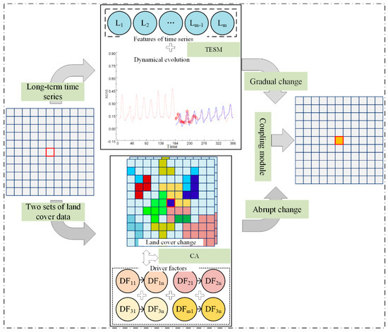
Figure 1.
The framework of the temporal dimension extension cellular automaton (TDE-CA). L and DF are the features and driving factors, respectively, used in the temporal evolution simulation module (TESM) and the CA (cellular automata) module.
2.1. The Temporal Evolution Simulation Module
Assuming that the climate changes and the interactions among various driving factors are stable. Land cover will evolve following the trends of the most recent period. Thus, it is reasonable for the TESM to simulate the dynamical evolution of land cover using the BFAST-monitor algorithm [41]. Then the dynamical characteristics of temporal evolution were converted to land cover types with SVMs (support vector machines) as the classifier.
2.1.1. The BFAST-Monitor
The BFAST-monitor algorithm introduces the CUSUM to extract a stable history period nearing the prediction period from the whole historical period [41]. The residual square sum (MOt) was selected as the discriminant basis in the CUSUM for the structural mutation of time series. If the MOt significantly deviates from 0 (p < 0.05), the algorithm will return the starting time of the stable historical period; otherwise, it will continue to move the sliding window (t = n, n − 1, n − 2, …, 1) until the first observation of time series. Figure 2 shows examples for pixel-based simulation of land cover evolution using the BFAST-monitor algorithm.
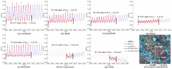
Figure 2.
The temporal evolutions of land cover types. R2 is correlation coefficient, stdev is the standard deviation, p is the significant level, the starting date 1 is the starting date of prediction period, the starting date 2 is the starting date of the stable period. Image in (h) is the false color composite (Bands 4, 3, and 2) synthetic SPOT image in 2015.
2.1.2. Classification
The dynamical characteristics of land cover evolution were converted to land cover types. Here, the SVM [43] was employed as the classifier for time series classification. The pseudo-invariant samples, selected by manual interpretation, were employed as the training samples in the SVM. Features play a key role in land cover classification. Thus, the phenological characteristics (including the start and end of growth-season, and duration) [44] and the Normalized Difference Vegetation Index (NDVI) time series in prediction year outputted from the BFAST-monitor [41] were extracted as classification features. In addition, the dynamic pattern and spatial cluster of time series were also considered as important attributes for vegetation classification [45]. Consequently, the change intensity, trend of the whole historical period, the fitting parameters, and the spatial cluster of fluctuation pattern in the stable historical period were also selected as classification features. Finally, the majority analysis was used to filter the salt and pepper classification noise, which often causes a fragmentation classification result [46].
2.2. The CA-Based Spatial Self-Organizing Simulation Module
Abrupt changes usually accompanied with a conversion of land cover type can be simulated by CA. Here, a constrained CA was used, which consisted of five elements: transition rules, neighborhood configuration, stochastic perturbation, constraints, and simulation time (time step). The transition rules are the core in CA models. The tree-based models, especially the RF generally, obtain more superior performance than statistical models in land cover simulation [25]. Thus, the RF was selected as transition rules in combination with CA.
However, the RF-CA still has many drawbacks. It is obvious that error accumulation exists in the RF-CA for using a series of static spatial variables to explain the occurrence-of-probability of land cover change over time [14].Correcting the probability-of-occurrence using updated driving factors may be an effective way to improve the performance of the RF-CA. Moreover, land cover and land use were influenced by the life-cycle of resource exploitation. During the different life-cycle phases, land use intensity and land demand are different. Markov chains model, a typical model for calculating conversion area, fails to predict the land cover change area among different life-cycle phases [31]. Thus, a conversion area coefficient should be employed to limit the conversion counts of land cover.
2.2.1. The Traditional RF-CA
The RF-CA is developed to simulate land cover under given time steps (iterations). It generally can be implemented in three steps. Firstly, the probability-of-occurrence of each land cover is estimated based on the RF. Then the combined probabilities of each land cover are calculated through combining the probability-of-occurrence with the neighborhood configuration, the stochastic perturbation, and the constraints. Thirdly, a self-adaptive conversion rules is designed to drive land cover conversion. The probability-of-occurrence Pg,ij of each pixel was adopted from [47]. Then the combined probabilities () of each land cover was represented as follows:
where t is the iteration number, is the neighborhood configuration with N number of pixels in the Moore neighborhood window [1], is the stochastic perturbation, which is determined by a random number (θ) that ranges from 0 to 1, and by a control parameter (λ) that ranges from 1 to 10. is the constraint, its value equal to 0 or 1. Specifically, we forbid the conversion of water, which means will equal 0 if the target cell is water and will otherwise equal 1.
Whether the original land cover type coverts to another land cover type is determined by a predefined threshold. The self-adaptive conversion rules can be expressed as follows:
where is the maximum value among , Kt is the predefined threshold which decreased with a special iterative decrease rate (rate), and the function max is a maximum value function.
2.2.2. Optimization of RF-CA
Under the driving of ever-changing factors, the probability-of-occurrence of each land cover types might change if the driven force is strong enough. We assumed that the probability-of-occurrence could be updated with a linear regression model if the updated driven factors were available. Least square regression was used to quantify the correlation between probability-of-occurrence and features. Pg,ij of the prediction phase was updated if the updated features existed, and the correlation between Pg and features were significant (evaluation indicators including correlation coefficient R2 and significance level p). The update function can be expressed as follows:
where Pug,ij means the updated probability-of-occurrence, which will replace Pg,ij in Equation (1) in calculating the combined probabilities; a and b represent the slope and the intercept, respectively, feature is the driven factors. The regression parameters were evaluated, using the pseudo-invariant samples as fitting samples.
An area correction coefficient r (r∈[0.5,1.5]) was introduced to correct the land cover area during different life-cycle phases. If the life cycle of the prediction period was the same as the simulation period, all the elements of r equal 1, and the conversion area of land cover would then be calculated by a Markov chains model; otherwise, at least one element never equals 1. The area correction formula is as follows:
where Asum is the total area, Msum is the area matrix outputted from Markov chains [48], m is the number of land cover, and r is the area correction coefficient. r is determined according to mineral resource exploitation planning documents and land reclamation planning documents in which the life cycle of resource exploitation and the reclamation contents (including location, area, and land cover type) are planned.
Through incorporating the area control strategy, Equation (2) can be changed as follows:
where the Areat is the total area of the land cover type with the max combined probabilities in t-th iteration.
2.3. Integrating Temporal Evolution Simulation Module with the Optimized RF-CA
Both gradual and abrupt changes were simulated by the TESM and the optimized RF-CA, respectively. However, these two simulation results suffered from different uncertainties and errors [14]. We sought a method to take full advantages of these two complementary simulation results for a comprehensive result, which is closer to the true land cover. EnKF (the ensemble Kalman filter) has been shown to be effective in coupling different results of land use change [14]. It can minimize the prediction uncertainties through assimilating the observation data into prediction results based on stochastic dynamic prediction theory. Usually, the EnKF model can be divided into two stages: a forecast phase and an analysis phase [49]. In the forecast phase, the forecast ensemble was randomly extracted from the results of a prediction model. Whereas in the analysis phase, the forecast ensemble was calibrated by the observation data ensemble, based on the minimum variance estimation method. Therefore, the EnKF was utilized to couple the two simulation results of land cover, using also the optimized RF-CA as the prediction model and the simulation results of the TESM as the observation data. The standard analysis formula of the EnKF is as follows:
where is the analysis field state variables ensemble, and B is the forecast field state variables ensemble predicted by the optimized RF-CA, which was then disturbed by Gauss noise. B = (b1, b2, …, bNum), Num means the size of the state variables ensemble,, is the mean of state variables, Q is the observation error covariance, and H is the observation operator linking the forecasting field states and the observation states. D is the observation variables ensemble which is perturbed by Gauss noise.
A development intensity (DI) was employed to convert discrete states of land cover into continuous states [14]. The DI calculation formula is as follows:
where M is the window size. After assimilation of the EnKF, the DI is converted into spatial cover type according to the integrated probability using the following formula:
where is the integration probability, is the land cover type conversion probability of the i-model, and wi is the weight coefficient; , in which Ji is the simulation error of the i-th model.
Figure 3 illustrates the schematic diagram of the assimilation process in the TDE-CA. The period between 2010 and 2015 is an example to explain the coupling mechanism. A five-year period was divided into five annual recursive phrases. In each recursive phrase, the TESM used the BFAST-monitor to extract the stable historical period (the blue hollow dots in Figure 3) from the whole historical time series ranging from 2000 to 2010 (the green solid line in Figure 3); the time series data was then used to fit and predict the time series in recursive phrase; finally, the TESM simulation results were converted to the DI as the observation state ensemble for the EnKF. On the other hand, the optimized RF-CA were operated independently to simulate land cover based on an initial land cover data; its simulation results were converted to the DI as the prediction state ensemble for the EnKF. Finally, the assimilation results were entered to the CA as the input data for the next recursive phase. Recurse until the end of the whole assimilation process.
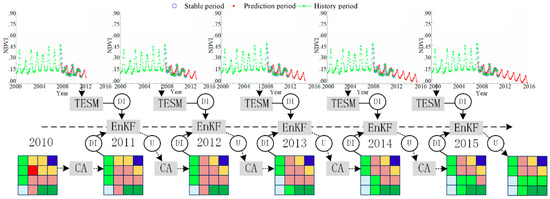
Figure 3.
The schematic diagram of the coupling module. Sparsely dotted arrows represent indirect input variables, solid arrows indicate directly input, and the medium dotted arrow is the timeline in the assimilation process.
2.4. Accuracy Assesment
The simulation results of the TDE-CA were respectively compared with a null model, with its sub-models (including the TESM and the optimized RF-CA), and with the traditional CA models (including the logistic-CA and the MLP-CA). Four strategies for model evaluation were selected to verify the effectiveness of the TDE-CA. Firstly, the grid cell level (AgreeGridcell), the agreement due to chance (AgreeChance), the agreement due to quantity (AgreeQuantity), the Kappa for no information (Kno), the Kappa for grid-cell level location (Klocation), and the traditional Kappa index of agreement (Kstandard) were selected as evaluation indicators to compare a null model with the TDE-CA [50]. Secondly, the user accuracy (UA), the producer accuracy (PA), the overall accuracy (OA), and the Kappa coefficient (Kappa) were used to compare the TDE-CA with its sub-models as well as with the traditional CA models in simulation accuracy [51]. Thirdly, partial enlargements of simulation results of the TDE-CA, the sub-models of TDE-CA, and the traditional CA models were compared with reference data to analyze the simulation performance in spatial distribution. Finally, five evaluation indicators related to the agreements and disagreements in location and quantity were selected to compare the TDE-CA with its sub-models, as well as with the traditional CA models. These five indicators included the disagreement due to quantity (DisagreeQuantity), the disagreement due to location at the grid cell level (DisagreeGridcell), AgreeGridcell, AgreeChance, and AgreeQuantity [52].
3. Study Area and Data Processing
3.1. Study Area
The Shendong coal mining area is one of the largest typical underground mining areas in China. It is in the contiguous area of the Shaanxi province and the Inner Mongolia, a typical ecologically fragile area. This area has a semi-arid climate; the perennial mean temperature, the average yearly precipitation, and the average annual evaporation are about 8.6 °C, 380 mm, and 2113 mm, respectively. Furthermore, the vegetation cover is sparse compared with mesic regions. On the other hand, due to the pressure of high-intensity mining and of other human activities, the landscape fragmentation of land cover is high, and land cover in this region changes frequently [45]. In this study, a 689 × 590-pixel area with 30 m spatial resolution per pixel was selected as the experiment area (Figure 4). This study site contains multiple minefields (such as the Majiata, Bulianta, Shangwan, Daliuta, Huojitu, and Zhugaita) and reserved lands, i.e., land acquired by coal enterprises in accordance with the law for early development or storage for future supply. The coordinates of the experimental site are from 39°13’57” N to 39°21’32” N, and from 110°12’33” E to 110°22’52” E. According to the field investigation of land cover types from 22 July to 27 July 2017 (illustrated by the black triangles in Figure 4), land cover includes mining pit, waste occupancy place, building, road, water, forest, desert forest, mixed forests, shrub, grassland, desert grassland, desert, cultivated land, and other types. Similar land cover was then incorporated to simplify the land cover categories. The mining pit, the waste occupancy place, buildings, and roads were merged into one land cover type named “developed land”; the forest, the desert forest, and the mixed forests collectively were referred to as “woodland”; both grassland and desert grassland were incorporated into the label “grassland”. Therefore, the following seven types of land cover were used in this paper: woodland, shrub, grassland, desert, farmland, water, and developed land.
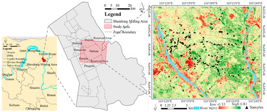
Figure 4.
Location of the study area in the Shendong mining area. The NDVI was calculated using Landsat imagery (30 July 2017). The black triangle shows the location of field investigation samples.
3.2. Data and Its Preprocessing
3.2.1. Remote Sensing Data for the Temporal Evolution Simulation Module
A total of 277 Level-1 Landsat images covering the period from 2000 to 2010 (Figure 5) were downloaded from the USGS (the U.S. Geological Survey) EROS (Earth Resources Observation and Science) Center to simulate the gradual change of land cover based on BFAST-monitor. The Level-1 Landsat images include TM and ETM+ products (WRS-2 path/row: 127/33). The LEDAPS (Landsat ecosystem disturbance adaptive processing system) was used to generate the surface reflectance products of TM and ETM+. Cloud, cloud shadow, and snow were masked from the Landsat images using the Fmask (function of mask) algorithm. In addition, Landsat L1T level images reached sub-pixel levels, indicating that Landsat does not need further geometric corrections [53]. However, to construct a 16-day-interval, high spatial resolution image time series, the STARFM (spatial and temporal adaptive reflectance fusion model) [54] and ESTARFM (the enhanced STARFM) [55] were utilized to generate Landsat-like images using the MCD43A4 as the coarse image (H/V:26/05, downloaded from https://ladsweb.modaps.eosdis.nasa.gov/). The NDVI was calculated to characterize the state of land cover dynamics. The self-adaptive Savitzky-Golay (S-G) filter [56] was then applied to reduce the noise of 30 m NDVI time series within a 16-day interval.
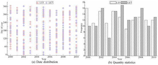
Figure 5.
All available Landsat images from 2000 to 2010. (a) Day of year distribution, and (b) the quantity statistics of Landsat images for each year.
To improve the reliability of the samples for time series classification, the SPOT images of 13 October 2004 and of 30 September 2011 were used as reference data to select pseudo-invariant samples as training samples. In addition, the embedded SPOT images with 1 scene on 21 September 2015 and two scenes on 5 October 2015 were selected as the reference data for cross-validation samples. All SPOT images were processed with orthorectification, layer stacking, merging, relative registration, and fusion. Table 1 shows the number of pseudo-invariant samples and cross-validation samples.

Table 1.
Pseudo-invariant samples and cross-validation samples.
3.2.2. Driving Factors for the CA-Based Spatial Self-Organizing Simulation Module
Considering the disturbance characteristics and the data availability of the Shendong coal mining area, the driving factors were divided into four major types: mining disturbance factors (MDF), surface habitat factors (SHF), artificial factors of land use (AFLU), and climatic factors (CF). The influence of the climatic factors is not only weak in terms of spatial variation but also already represented by the evolution of land cover itself. For these reasons, the climatic factors were excluded from the index system. A total of 20 driving factors were selected as feature variables to calculate the probability of occurrence. All factors derived from the original datasets are listed in Table 2; they were normalized in the range [0,1], and resampled to a 30 × 30 m2 spatial resolution.
Table 2.
Driving factors for the calculation of probability-of-occurrence.
4. Results
4.1. Model Initialization and Parameter Setteing
The TDE-CA was tested in the Shendong mining area, setting the year 2015 as the forecast year, and taking land cover sets in 2005 and 2010 as historical reference data for the optimized RF-CA. These two historical reference data were extracted from Landsat images. The classification accuracy of the OA and Kappa were 92.60% and 0.9103 in 2005, respectively, and 88.91% and 0.8628 in 2010, respectively. For the TESM, the NDVI time series with a 30 m spatial solution and 16-day interval from 2000 to 2010 was set as the historical time series in BFAST-monitor to simulate the evolution of land cover. The parameters used in the TDE-CA are shown in Table 3. The determination of these parameters is partly based on the combination of pre-estimation and post-calibration.
Table 3.
Parameters used in the TDE-CA which were organized by different modules.
4.2. Comparison of the TDE-CA and a Null Model
A strong agreement between a predicted map and a reference map does not necessarily demonstrate the good performance of a model; however, the higher agreement of a model compared with a null model is the necessary condition for a valid model [52]. A null model is the scientist’s best prediction according to the historical land cover, without using a simulation model. This paper compared the simulation results of the TDE-CA in 2015 with a null model, where the null model takes the land cover in 2010 as its prediction results. Table 4 shows the evaluation indicators in terms of change, quantity, location, and accuracy at grid cell level calculated by using the IDRISI® (J. Ronald Eastman, Clark Labs, Clark University, Worcester, Massachusetts, USA). The results indicate that the AgreeChance, AgreeQuantity, and AgreeGridcell of the TDE-CA were higher than the null model. This shows that the TDE-CA is better than the null model in simulating change, quantity, and location of land cover. In addition, Kno, Klocation, and Kstandard also provided favorable evidence for the effectiveness of the TDE-CA. These three accuracy indicators exhibited similar values to earlier results, with Kno ranging from 0.63 to 0.77, Klocation ranging from 0.69 to 0.80, and Kstandard ranging from 0.74 to 0.92 [58]. Additionally, as concluded by Koomen (2008), LUCC simulation models are more accurate than their corresponding null model at pixel resolution. The LUCC model must be more accurate than its null model also at the coarsest resolution [51]. Therefore, the TDE-CA can be a valid model for land cover simulation both at pixel and coarse resolution levels.
Table 4.
Comparison of the null model and the TDE-CA.
4.3. Comparison of the TDE-CA and its Sub-Models
4.3.1. Comparison of the TDE-CA and its Sub-Models in Accuracy
The TDE-CA can effectively improve the performances of land cover simulation by simultaneously simulating spatial-led abrupt change and temporal-led gradual change [59]. Table 5 shows the results of simulation accuracy of the TDE-CA and its sub-models. Compared to its sub-models, the TDE-CA achieved the highest accuracy in both OA and Kappa, with a respective increase of 17.84% and 21.67% when compared with the TESM, and of 4.48% and 5.12% when compared with the optimized RF-CA. When compared with the optimized RF-CA, the TDE-CA achieved the highest UAs in the land types with vegetation cover including woodland, shrub, grassland, and farmland, and the worst UAs in the land types with non-vegetation cover including desert, developed land, and water. Such results indicate that, by integrating the evolution of land cover (simulated by TESM) with the intrinsically spatial evolution (simulated by optimized RF-CA), UAs can be an effective strategy to improve the simulation accuracy of vegetation coverage area. It is also a desirable solution for the simulation of a complex system by coupling multi-processes or multi-models [1,15,32].
Table 5.
The accuracies comparison of the TDE-CA and its sub-models.
4.3.2. Comparison of the TDE-CA and Sub-Models in Spatial Pattern
Figure 6 shows the spatial distribution of land cover in 2015 simulated by the TDE-CA, and the sub-models of the TDE-CA. To display more details of the simulation results, three partial enlargements were used to compare the simulation results with the actual land cover. These three partial enlargements of the actual land cover were generated by visually interpreting the SPOT images in 2015. The results indicate that the TDE-CA not only inherit the spatial detail information from the TESM, but also inherit the plaque aggregation from the optimized RF-CA. Additionally, the TDE-CA is more consistent with the actual land cover than its sub-models (the first enlargements in Figure 6), which is especially obvious when compared with the optimized RF-CA (the second and third enlargements in Figure 6). Compared with the actual land cover, the simulation results of the TDE-CA and the optimized RF-CA are more aggregated, while the simulation results of the TESM are more fragmented. This aggregation in space of the cell-based CA could be attributed to the neighborhood configuration which only stress the edge-expansion growth of land cover, yet overlook the stochastic growth.
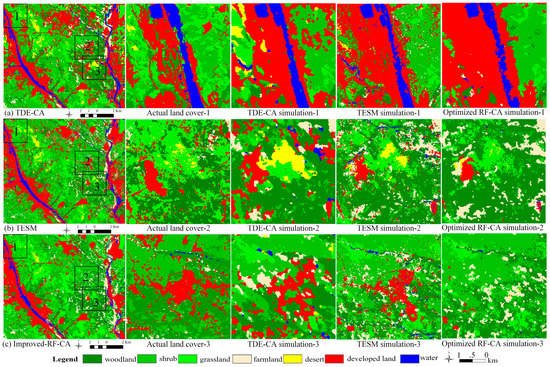
Figure 6.
The spatial distribution and partial enlargements of land cover. (a–c) respectively present the land cover simulation of the TDE-CA, the TESM, and the optimized RF-CA.
4.3.3. Comparison of the TDE-CA and Sub-Models in Agreements and Disagreements
The comparison of the simulation accuracy and the spatial pattern between the TDE-CA and its sub-models demonstrate that integrating the TESM with CA can theoretically expand CA from instantaneous to continuous simulation and can simultaneously improve the simulation performance. However, criticisms of the error matrix (a specific table layout that allows visualization of the performance of an algorithm) and the qualitative analysis include that they do not quantitively account for the spatial agreements and disagreements on one hand and that they fail to account for random agreements on the other. Hence, the error budget method was used to perform an additional evaluation taking the DisagreeQuantity, DisagreeGridcell, AgreeGridcell, AgreeChance, and AgreeQuantity as the evaluation indicators.
Figure 7 shows that the DisagreeQuantity of the TDE-CA was lower than for the TESM and for the optimized RF-CA. Conversely, the AgreeGridCell and the AgreeQuantity of the TDE-CA were higher. These results demonstrate the higher quantity and location accuracy of the TDE-CA compared to its sub-models, which is due to the extension of the CA with the temporal evolution of land cover. Moreover, by simultaneously considering the spatial and temporal processes, the TDE-CA tends to achieve more robust and accurate results for land use and land cover simulation [59]. Although the improvements of the agreement in quantity and location have been proved, the DisgreeGridcell of the TDE-CA showed almost no improvement compared with the TESM, and was even lower than for the optimized RF-CA. This result can be attributed to the high spatial heterogeneity of the landscape in the study area, and to the extent of change of the cell states. Under the pressure of high-intensity mining and of other human activities, the land cover rapidly changed from one type to another. As a result, it is difficult for the TESM to capture the high location agreement and the change agreements during the predicted period. Hence, a fine spatial resolution and nonlinear models are desirable to improve the performance of the TESM simulation [18,60].
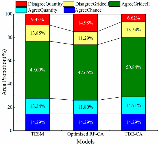
Figure 7.
The comparison of the TDE-CA and its sub-models in agreement and disagreement.
4.4. Comparison of the TDE-CA and Other Simulation Models
4.4.1. Comparison of the TDE-CA and Other Models in Accuracy
The logistic-CA [22] and the MLP-CA [23] were also run to make a comparison with the TDE-CA; the training data and the driving factors were the same as for the optimized RF-CA. Table 6 displays the simulation accuracy of each model. Compared to traditional CA models, the TDE-CA achieved the highest accuracy in both OA and Kappa with a respective increase of 8.41% and 0.0985, when compared with the logistic-CA, and of 8.28% and 0.0961 when compared with the MLP-CA. Although the TDE-CA significantly improved compared to both the logistic-CA and the MLP-CA, the OA and Kappa still did not reach the desired level for application [48]. One of the reasons for this result might be the substantial and disordered land cover change in the mining area, which was directly or indirectly affected by underground mining, surface habitat, land exploitation and utilization, and climate change [61]. Previous studies have shown that the rates of land cover change in the mining area can vary even over a short time period [45]. As a result, multiple time periods should be considered when predicting future land cover in those areas that are under high-intensity development [14]. Existing mature, two-period-based simulation models, like the logistic-CA and the MLP-CA, which already proved to have a high performance in land cover simulation [22,23], failed to have a perfect performance in this study area. On the other hand, previous studies proved that the introduction of information on multiple time periods avoids the error accumulation, by calibrating the parameters in the model [14].
Table 6.
Comparison of the TDE-CA and other models in simulation accuracy.
When compared with both the logistic-CA and the MLP-CA, the TDE-CA achieved the highest UAs in the land types with vegetation cover including woodland, shrub, grassland, and farmland, and the worst PAs in these same land types except for farmland. On the contrary, the non-vegetation cover types of TDE-CA gained the highest PAs. The lower PAs of the TDE-CA in vegetation cover types, compared to other models, might be attributed to the potential errors generated by the TESM module, which assumes an evolution of land cover at current trends, according to a stable historical time series [41]. This hypothesis led to the evolution of a vegetation type with indirect disturbance into a non-vegetation type. On the other hand, the growth and succession of vegetation in real life is a slow process, especially in arid and semi-arid ecologically fragile areas. Contrary to the evolution of vegetation, the non-vegetation types with a weak or even no evolution trend did not change the results in the model simulation [52]. As a result, the area of vegetation type may be underestimated, while the non-vegetation type may be overestimated. One of the possible solutions to this problem is to use long-term and fine spatial resolution time series to simulate the temporal evolution, so that potential errors may be effectively controlled [62]. Another possible solution is to use a depth learn framework to learning the feedback mechanisms between the temporal evolution and the driving factors [18,60].
4.4.2. Comparison of the TDE-CA and Other Models in Spatial Pattern
Figure 8 shows the simulation results of the logistic-CA, the MLP-CA, and the TDE-CA, as well as its three partial enlargements and the actual land cover pattern. From a global perspective (Figure 8a-c), the TDE-CA is effective in simulating both edge-expansion growth and outlying stochastic growth, but the cell-based logistic-CA and MLP-CA can just simulate edge-expansion growth. These comparison results indicate that a pixel-based land cover evolution module in CA can increase the possibility of stochastic growth for land cover. More detailed information in the three partial enlargements also confirm the above indication (the first and second enlargements in Figure 8). The simulation result of the TDE-CA is more consistent with the actual land cover than the logistic-CA and the MLP-CA, which is especially obvious in developed land and farmland. Additionally, the TDE-CA, the logistic-CA, and the MLP-CA failed to simulate the spatial distribution of linear land cover types (the third enlargements in Figure 8), which suggest that additional improvements should be considered. Meetemeyer (2013) proposed a multilevel modeling framework by combining the field-based and the object-based presentations of the land cover change, which overall considers the size, shape, and structure of land spatial evolution, potentially solving the linear expansion problem [63].
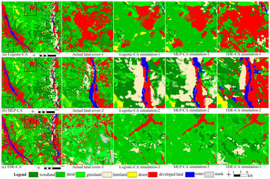
Figure 8.
The spatial distribution of land cover of different CA models. (a–c) respectively present simulation results of the logistic-CA, the MLP-CA, and the TDE-CA.
4.4.3. Comparison of the TDE-CA and Other Models in Agreements and Disagreements
In this section, we present the results of the analysis of agreement and disagreement in quantity and location of the simulation results for 2015, by using the error budget method. As shown in Figure 9, the quantitative consistency of the TDE-CA was significantly enhanced in comparison with the other models, with a reduction of nearly 10% in the DisagreeQuantity, and an increase in AgreeGridcell of 3.78% and 3.71% when compared with the logistic-CA and the MLP-CA. Compared with the traditional CA, which only emphasizes the process of spatial self-organization, the addition of the land cover evolution process can effectively improve the quantitative consistency of land cover simulation. This conclusion also illustrates the superiority of coupling multiple process models [58]. If we compare the location agreement and disagreement of the TDE-CA with the logistic-CA and the MLP-CA, we can see that the AgreeGridcell of the TDE-CA increased by 4.69% and 4.49%, respectively. However, the DisagreeGridcell of the TDE-CA obtained a lower result than for the two traditional CA models; this indicates that the TDE-CA should be further fixed by rearranging the predicted pixel in space [52].
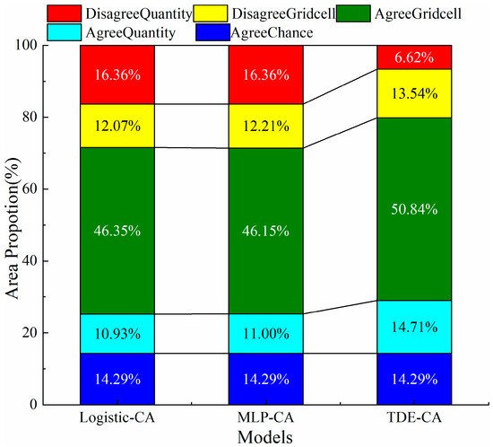
Figure 9.
The comparison of the TDE-CA and other models in agreement and disagreement.
5. Discussion
5.1. Parameter Sensitivity Analysis
Although fully considering the process characteristics of land cover change, the TDE-CA simulation results are still affected by multiple parameters, including the neighborhood configuration and the number of iterations. The neighborhood configuration reflects the spatial disturbance intensity and the radiation range, while the number of iterations in the RF-CA directly affects the local spatial competition intensity. Thus, to explore the influence of neighborhood on model accuracy and to reduce the uncertainty of the model, the simulation accuracy (including OA and Kappa) of the RF-CA with different Moore neighborhood windows (3 × 3, 5 × 5, 7 × 7, and 9 × 9) was analyzed. The results show that both the OA and Kappa decrease with the increase of the neighborhood windows (Table 7). A 3 × 3 Moore neighborhood window appears to be the most suitable window size for the RF-CA in the Shengdong mining area. Relatively few iterations lead to insufficient land cover space interactions, while a disproportionate amount of iterations are prone to excessive expansion or contraction in the simulation [11]. Table 7 shows the OA and Kappa of the RF-CA declined with increasing iterations.
Table 7.
The simulation accuracy of different neighborhood windows and a different number of iterations.
In addition, to verify the effectiveness of the optimizations in the RF-CA, the OA, and the Kappa of the RF-CA and of the optimized RF-CA were tested with (or without) a feature update and with (or without) the area control. The comparative results show that the introduction of the feature update and of the area control further improved the precision of the RF-CA simulation (Table 8). The OA and the Kappa were, respectively, 5.72% and 0.0678 higher than the RF-CA. These results indicate that the feature update and the area control can provide an opportunity to improve the accuracy of results of the traditional CA.
Table 8.
The accuracy of the corrections with or without a feature update and area control.
5.2. Advantages and Adaptability of the TDE-CA
Land cover simulation models are required to fulfill two main needs. The first one is to explain complex land cover changes, including both gradual and abrupt change under the action of multiple driving factors. The second is to quantify the correlation between the driving factors and land cover change with unknown driving mechanisms. These requirements make the usage of a traditional model to simulate land cover with high-precision rather difficult. Fortunately, the detailed characterization of land cover change has become possible due to the development of earth observation technology, the accumulation of remote sensing data, and the free opening of remote sensing history archives [55]. Thus, the TDE-CA was proposed based on the temporal dimension extension. Results demonstrate that the integration of gradual land cover change into the CA can effectively extend the spatial-temporal scale from instantaneous to continuous simulation and can simultaneously improve simulation precision. Further improvements were implemented to improve the consistency of the single process simulation with land cover change. In relation to the dynamic process simulation, the BFAST-monitor was chosen to detect a stable history period to replace the all of the historical data in the fitting time series. The BFAST-monitor achieved a high score in the fitness tests for each land cover type; thus, it can effectively avoid the fitting deviation in multiple change patterns based on stable history periods [37,41]. In relation to the spatial abrupt change, the RF-CA proved to have a high robustness and anti-overfitting in land cover simulation with unknown driving mechanisms [17,25]. As a result, the TDE-CA can simulate not only the spatial self-organizing process of land cover but also the long-term weak change of land cover caused by land degradation, desertification, afforestation, or other indirect effects of human activities.
5.3. Limitations and Future Work
Although the TDE-CA and some of its parameters have been validated and analyzed, it is worth mentioning that the application of the TDE-CA still has some limitations. Affected by sensor technology and cloud pollution, the long-term NDVI time series with dual high resolution (i.e., high time resolution and high spatial resolution) is scarce [55]. This paper blends 75 scene images in the Landsat time series for the period from 2000 to 2010, using spatiotemporal fusion algorithms (including the STARFM [54] and the ESTARFM [55]). In more detail, 50 scenes were fused with the STARFM, and 19 scenes were fused with the ESTARFM, while 6 scenes could not be generated by neither the STARFM nor the ESTARFM. Nevertheless, the noise information in the fusion image increased the uncertainty of the TESM. Supplementary research should seek to improve the spatiotemporal fusion algorithm or develop a new one. Moreover, the image time series construction method with multi-platform and multi-data sources should be investigated to reduce the uncertainty of the data [64]. The limitation of the model related to spatial abrupt change emerged from the consideration of two aspects. The first is the facility to generate error accumulation from change detection based on the classification of remote sensing [14]. The second aspect is the difficulty for the traditional pixel-based CA (generally edge-expansion) to simulate an edge-expansion growth [16,65]. Promising strategies to solve these problems in the traditional pixel-based CA include extracting the changed land cover using multispectral change detection instead of performing a post-classification comparison [14,26], and expressing the cell unit with an object-based unit instead of a pixel-based cell unit in cellular automata [16,21]. Even though model coupling can effectively improve the precision of land cover simulation, there are still high uncertainties in the development strength and in category mapping. Those uncertainties are also a potential block for the high robustness of simulation models [65]. In relation to the application, even if the TDE-CA achieved a good accuracy, its suitability for other simulation systems would need further verification and analysis. Finally, it is clear that the increase in the embedding of both process and module, if compared to the traditional CA, implies the increase in the uncertainty of the model, as shown by the exponential increase of parameters of the TDE-CA parameters if compared with both the logistic-CA and the MLP-CA.
6. Conclusions
CA models, based on the comparison of the sets at the beginning and at the end of the training period, are inappropriate for depicting the dynamic process of land cover. In fact, CA models fail to explain the long-term evolution of land cover, as well as to accurately predict land cover. To solve this problem, this study proposed the TDE-CA by integrating the temporal evolution of land cover with the intrinsically spatial evolution of CA, based on assimilation theory. The TDE-CA was applied to investigate the case of the Shendong mining area. The simulation results of the TDE-CA were compared with the simulation results of a null model, of the sub-models of the TDE-CA, and of other traditional CA models including the logistic-CA and the MLP-CA. Results show that the integration of the temporal evolution of land cover with CA can extend the spatial-temporal scale of the CA model from instantaneous to continuous simulation. This in turn provides a feasible method for long-term land cover simulation. The comparison of the TDE-CA with its sub-models and with other traditional CA models shows that the TDE-CA is superior to its sub-models and to the traditional CA models in terms of both simulation accuracy and quantity allocation. However, some potential limitations are worth noting. Although the proposed TDE-CA was shown to be effective to improve quantitative accuracy compared with other traditional CA models, the disagreement due to the location at grid cell level is still high. This aspect could be fixed in the future by rearranging the predicted pixels in space. Moreover, the TDE-CA was tested only with a stable historical time series; further simulation with the longer series of data should be performed to test the performance of this model.
Author Contributions
C.W., S.L., and D.J. had the original idea for the study; C.W. and D.J. conceived and designed the experiments; C.W. performed the experiments; all co-authors interpreted the results; S.L., D.J., and S.M. contributed reagents/materials/analysis tools; C.W. drafted the manuscript, which was then improved and revised by S.L. and A.J.E.; S.L., A.J.E., and S.M. offered guidance and supervision. All authors read and approved the final manuscript.
Funding
This research was funded by the National Key Research and Development Program, grant number 2016YFC0501107, and by the Special Project of Science and Technology Basic Work of Ministry of Science and Technology of China, grant number, 2014FY11080.
Acknowledgments
This research was funded by the National Key Research and Development Program, grant number 2016YFC0501107, and by the Special Project of Science and Technology Basic Work of Ministry of Science and Technology of China, grant number 2014FY110800. We would like to thank the anonymous reviewers for providing us with useful comments and suggestions, which helped us to improve the quality of this manuscript.
Conflicts of Interest
The authors declare no conflict of interest.
References
- Liu, X.; Liang, X.; Li, X.; Xu, X.; Ou, J.; Chen, Y.; Li, S.; Wang, S.; Pei, F. A future land use simulation model (FLUS) for simulating multiple land use scenarios by coupling human and natural effects. Landsc. Urban Plan. 2017, 168, 94–116. [Google Scholar] [CrossRef]
- Luo, B.; Li, J.B.; Huang, G.H.; Li, H.L. A simulation-based interval two-stage stochastic model for agricultural non-point source pollution control through land retirement. Sci. Total Environ. 2006, 361, 38–56. [Google Scholar] [CrossRef] [PubMed]
- Vogelmann, J.E.; Gallant, A.L.; Shi, H.; Zhu, Z. Perspectives on monitoring gradual change across the continuity of Landsat sensors using time-series data. Remote Sens. Environ. 2016, 185, 258–270. [Google Scholar] [CrossRef]
- Arsanjani, J.J. Characterizing, monitoring, and simulating land cover dynamics using GlobeLand30: A case study from 2000 to 2030. J. Environ. Manag. 2018, 214, 66–75. [Google Scholar] [CrossRef] [PubMed]
- Brown, D.; Band, L.E.; Green, K.O.; Irwin, E.G.; Jain, A.; Lambin, E.F.; Pontius, R.G.; Seto, K.C.; Turner, B.L., II; Verburg, P.H. Advancing Land Change Modeling: Opportunities and Research Requirements; The National Research Council Press: Washington, DC, USA, 2013; ISBN 9780309288330. [Google Scholar]
- Wolfram, S. Cellular automata as models of complexity. Nature 1984, 311, 419–424. [Google Scholar] [CrossRef]
- Salhab, R.; Malhamé, R.P.; Ny, J.L. A Dynamic Game Model of Collective Choice in Multiagent Systems. In Proceedings of the IEEE Conference on Decision and Control, Osaka, Japan, 15–18 December 2015; pp. 4444–4449. [Google Scholar]
- Shang, C.; Fang, H.; Chen, J.; Zhang, J. Interacting with multi-agent systems through intention field based shared control methods. In Proceedings of the Asian Control Conference, Gold Coast, QLD, Australia, 17–20 December 2017; pp. 150–155. [Google Scholar]
- Parker, D.C.; Manson, S.M.; Janssen, M.A.; Hoffmann, M.J.; Deadman, P. Multi-Agent Systems for the Simulation of Land-Use and Land-Cover Change: A review. Ann. Assoc. Am. Geogr. 2015, 93, 314–337. [Google Scholar] [CrossRef]
- Zhang, P.; Gong, M.; Su, L.; Liu, J.; Li, Z. Change detection based on deep feature representation and mapping transformation for multi-spatial-resolution remote sensing images. ISPRS J. Photogramm. Remote Sens. 2016, 116, 24–41. [Google Scholar] [CrossRef]
- Jiang, X.; Lin, M.; Zhao, J. Woodland Cover Change Assessment Using Decision Trees, Support Vector Machines and Artificial Neural Networks Classification Algorithms. In Proceedings of the 4th International Conference on Intelligent Computation Technology and Automation, Shenzhen, China, 28–29 March 2011; pp. 312–315. [Google Scholar]
- Basse, R.M.; Charif, O.; Bódis, K. Spatial and temporal dimensions of land use change in cross border region of Luxembourg. Development of a hybrid approach integrating GIS, cellular automata and decision learning tree models. Appl. Geogr. 2016, 67, 94–108. [Google Scholar]
- Samardzic-Petrovic, M.; Kovačević, M.; Bajat, B.; Dragicevic, S. Machine Learning Techniques for Modelling Short Term Land-Use Change. ISPRS Int. J. Geo-Inf. 2017, 6, 387. [Google Scholar] [CrossRef]
- Li, X.; Zhang, Y.; Liu, X.; Chen, Y. Assimilating process context information of cellular automata into change detection for monitoring land use changes. Int. J. Geogr. Inf. Sci. 2012, 26, 1667–1687. [Google Scholar] [CrossRef]
- Lauf, S.; Haase, D.; Hostert, P.; Lakes, T.; Kleinschmit, B. Uncovering land-use dynamics driven by human decision-making—A combined model approach using cellular automata and system dynamics. Environ. Model. Softw. 2012, 27–28, 71–82. [Google Scholar] [CrossRef]
- Moreno, N.; Wang, F.; Marceau, D.J. Implementation of a dynamic neighborhood in a land-use vector-based cellular automata model. Comput. Environ. Urban Syst. 2009, 33, 44–54. [Google Scholar] [CrossRef]
- Li, X.; Liu, X.; Yu, L. A systematic sensitivity analysis of constrained cellular automata model for urban growth simulation based on different transition rules. Int. J. Geogr. Inf. Sci. 2014, 28, 1317–1335. [Google Scholar] [CrossRef]
- Liang, X.; Liu, X.; Li, X.; Chen, Y.; Tian, H.; Yao, Y. Delineating multi-scenario urban growth boundaries with a CA-based FLUS model and morphological method. Landsc. Urban Plan. 2018, 177, 47–63. [Google Scholar] [CrossRef]
- Li, X.; Chen, Y.; Liu, X.; Li, D.; He, J. Concepts, methodologies, and tools of an integrated geographical simulation and optimization system. Int. J. Geogr. Inf. Sci. 2011, 25, 633–655. [Google Scholar] [CrossRef]
- Li, X.; Yeh, G.O. Calibration of Cellular Automata by Using Neural Networks for the Simulation of Complex Urban Systems. Environ. Plan. A 2001, 33, 1445–1462. [Google Scholar] [CrossRef]
- Liu, X.; Ma, L.; Li, X.; Ai, B.; Li, S.; He, Z. Simulating urban growth by integrating landscape expansion index (LEI) and cellular automata. Int. J. Geogr. Inf. Sci. 2014, 28, 148–163. [Google Scholar] [CrossRef]
- Fulong, W. Calibration of stochastic cellular automata: the application to rural-urban land conversions. Int. J. Geogr. Inf. Syst. 2002, 16, 795–818. [Google Scholar]
- Ozturk, D. Urban Growth Simulation of Atakum (Samsun, Turkey) Using Cellular Automata-Markov Chain and Multi-Layer Perceptron-Markov Chain Models. Remote Sens. 2015, 7, 5918–5950. [Google Scholar] [CrossRef]
- Yang, Q.; Li, X.; Shi, X. Cellular automata for simulating land use changes based on support vector machines. Comput. Geosci. 2006, 34, 592–602. [Google Scholar] [CrossRef]
- Kamusoko, C.; Gamba, J. Simulating Urban Growth Using a Random Forest-Cellular Automata (RF-CA) Model. ISPRS Int. J. Geo-Inform. 2015, 4, 447–470. [Google Scholar] [CrossRef]
- Chen, Y.; Li, X.; Liu, X.; Ai, B.; Li, S. Capturing the varying effects of driving forces over time for the simulation of urban growth by using survival analysis and cellular automata. Landsc. Urban Plan. 2016, 152, 59–71. [Google Scholar] [CrossRef]
- Feng, Y.; Liu, Y.; Tong, X.; Liu, M.; Deng, S. Modeling dynamic urban growth using cellular automata and particle swarm optimization rules. Landsc. Urban Plan. 2011, 102, 188–196. [Google Scholar] [CrossRef]
- Aburas, M.M.; Ho, Y.M.; Ramli, M.F.; Ash’Aari, Z.H. The simulation and prediction of spatio-temporal urban growth trends using cellular automata models: A review. Int. J. Appl. Earth. Obs. Geoinf. 2016, 52, 380–389. [Google Scholar] [CrossRef]
- Rienow, A.; Goetzke, R. Supporting SLEUTH—Enhancing a cellular automaton with support vector machines for urban growth modeling. Comput. Environ. Urban Syst. 2015, 49, 66–81. [Google Scholar] [CrossRef]
- Xu, Z.; Coors, V. Combining system dynamics model, GIS and 3D visualization in sustainability assessment of urban residential development. Build. Environ. 2012, 47, 272–287. [Google Scholar] [CrossRef]
- Moghadam, H.S.; Helbich, M. Spatiotemporal urbanization processes in the megacity of Mumbai, India: A Markov chains-cellular automata urban growth model. Appl. Geogr. 2013, 40, 140–149. [Google Scholar]
- Candau, J.; Rasmussen, S.; Clarke, K.C. A coupled cellular automaton model for land use/land cover dynamics. In Proceedings of the 4th International Conference on Integrating GIS and Environmental Modeling (GIS/EM4): Problems, Prospects and Research Needs, Banff, AB, Canada, 2–8 September 2000; pp. 2–8. [Google Scholar]
- Xu, X.; Du, Z.; Zhang, H. Integrating the system dynamic and cellular automata models to predict land use and land cover change. Int. J. Appl. Earth. Obs. Geoinf. 2016, 52, 568–579. [Google Scholar] [CrossRef]
- Li, W.; Wu, C.; Zang, S. Modeling urban land use conversion of Daqing City, China: a comparative analysis of “top-down” and “bottom-up” approaches. Stoch. Environ. Res. Risk Assess. 2014, 28, 817–828. [Google Scholar] [CrossRef]
- Herold, M. Spatio-temporal dynamics in California’s Central Valley: Empirical links to urban theory. Int. J. Geogr. Inf. Sci. 2005, 19, 175–195. [Google Scholar]
- Gómez, C.; White, J.C.; Wulder, M.A. Optical remotely sensed time series data for land cover classification: A review. ISPRS J. Photogramm. Remote Sens. 2016, 116, 55–72. [Google Scholar] [CrossRef]
- Zhu, Z.; Fu, Y.; Woodcock, C.E.; Olofsson, P.; Vogelmann, J.E.; Holden, C.; Wang, M.; Dai, S.; Yu, Y. Including land cover change in analysis of greenness trends using all available Landsat 5, 7, and 8 images: A case study from Guangzhou, China (2000–2014). Remote Sens. Environ. 2016, 185, 243–257. [Google Scholar] [CrossRef]
- Zhu, Z.; Woodcock, C.E.; Olofsson, P. Continuous monitoring of forest disturbance using all available Landsat imagery. Remote Sens. Environ. 2012, 122, 75–91. [Google Scholar] [CrossRef]
- Kennedy, R.E.; Yang, Z.; Cohen, W.B. Detecting trends in forest disturbance and recovery using yearly Landsat time series: 1. LandTrendr—Temporal segmentation algorithms. Remote Sens. Environ. 2010, 114, 2897–2910. [Google Scholar] [CrossRef]
- Zhu, Z.; Woodcock, C.E. Continuous change detection and classification of land cover using all available Landsat data. Remote Sens. Environ. 2014, 144, 152–171. [Google Scholar] [CrossRef]
- Verbesselt, J.; Zeileis, A.; Herold, M. Near real-time disturbance detection using satellite image time series. Remote Sens. Environ. 2012, 123, 98–108. [Google Scholar] [CrossRef]
- Ding, J.; Zhou, J.; Tarokh, V. Optimal prediction of data with unknown abrupt change points. In Proceedings of the IEEE Global Conference on Signal and Information Processing (GlobalSIP), Montreal, QC, Canada, 14–16 November 2017; pp. 928–932. [Google Scholar]
- Chang, C.C.; Lin, C.J. LIBSVM:a library for support vector machines. ACM TIST 2011, 2, 1–27. [Google Scholar] [CrossRef]
- Jonsson, P.; Eklundh, L. Seasonality extraction by function fitting to time-series of satellite sensor data. IEEE Trans. Geosci. Remote Sens. 2002, 40, 1824–1832. [Google Scholar] [CrossRef]
- Jia, D.; Wang, C.; Lei, S. Semisupervised GDTW kernel-based fuzzy c-means algorithm for mapping vegetation dynamics in mining region using normalized difference vegetation index time series. J. Appl. Remote Sens. 2018, 12, 1. [Google Scholar] [CrossRef]
- Chen, C.; Wang, J.; Qin, W.; Dong, X. A new adaptive weight algorithm for salt and pepper noise removal. In Proceedings of the 2011 International Conference on Consumer Electronics, Communications and Networks (CECNet), Xianning, China, 16–18 April 2011; pp. 26–29. [Google Scholar]
- Breiman, L. Random Forests. Mach. Learn. 2001, 45, 5–32. [Google Scholar] [CrossRef]
- Erna, L.; Gerardo, B.; Manuel, M.; Emilio, D. Predicting land-cover and land-use change in the urban fringe: A case in Morelia city, Mexico. Landsc. Urban Plan. 2001, 55, 271–285. [Google Scholar]
- Evensen, G. The Ensemble Kalman Filter: theoretical formulation and practical implementation. Ocean Dyn. 2003, 53, 343–367. [Google Scholar] [CrossRef]
- Pontius, R.G.P.J.; Millones, M. Death to Kappa: birth of quantity disagreement and allocation disagreement for accuracy assessment. Int. J. Remote Sens. 2011, 32, 4407–4429. [Google Scholar] [CrossRef]
- Pontius, R.G.P.J.; Boersma, W.; Castella, J.-C.; Clarke, K.; de Nijs, T.; Dietzel, C.; Duan, Z.; Fotsing, E.; Goldstein, N.; Kok, K.; et al. Comparing the input, output, and validation maps for several models of land change. Ann. Reg. Sci. 2008, 42, 11–37. [Google Scholar] [CrossRef]
- Pontius, R.G.P.J.; Huffaker, D.; Denman, K. Useful techniques of validation for spatially explicit land-change models. Ecol. Model. 2004, 179, 445–461. [Google Scholar] [CrossRef]
- Emelyanova, I.V.; Mcvicar, T.R.; Niel, T.G.V.; Li, L.T.; Dijk, A.I.J.M.V. Assessing the accuracy of blending Landsat–MODIS surface reflectances in two landscapes with contrasting spatial and temporal dynamics: A framework for algorithm selection. Remote Sens. Environ. 2013, 133, 193–209. [Google Scholar] [CrossRef]
- Gao, F.; Masek, J.; Schwaller, M.; Hall, F. On the blending of the Landsat and MODIS surface reflectance: predicting daily Landsat surface reflectance. IEEE Trans. Geosci. Remote Sens. 2006, 44, 2207–2218. [Google Scholar]
- Zhu, X.L.; Jin, C.; Feng, G.; Chen, X.H.; Masek, J.G. An enhanced spatial and temporal adaptive reflectance fusion model for complex heterogeneous regions. Remote Sens. Environ. 2010, 114, 2610–2623. [Google Scholar] [CrossRef]
- Chen, J.; Jönsson, P.; Tamura, M.; Gu, Z.; Matsushita, B.; Eklundh, L. A simple method for reconstructing a high-quality NDVI time-series data set based on the Savitzky–Golay filter. Remote Sens. Environ. 2004, 91, 332–344. [Google Scholar] [CrossRef]
- Liu, Q.; Liu, G.; Huang, C.; Liu, S.; Zhao, J. A tasseled cap transformation for Landsat 8 OLI TOA reflectance images. In Proceedings of the 2014 IEEE Geoscience and Remote Sensing Symposium, Quebec City, QC, Canada, 13–18 July 2014; pp. 541–544. [Google Scholar]
- Hepinstall, J.A.; Alberti, M.; Marzluff, J.M. Predicting land cover change and avian community responses in rapidly urbanizing environments. Landsc. Ecol. 2008, 23, 1257–1276. [Google Scholar] [CrossRef]
- Schröder, B.; Seppelt, R. Analysis of pattern–process interactions based on landscape models—Overview, general concepts, and methodological issues. Ecol. Model. 2006, 199, 505–516. [Google Scholar] [CrossRef]
- Liu, X.; Ou, J.; Li, X.; Ai, B. Combining system dynamics and hybrid particle swarm optimization for land use allocation. Ecol. Model. 2013, 257, 11–24. [Google Scholar] [CrossRef]
- Lei, S.; Ren, L.; Bian, Z. Time–space characterization of vegetation in a semiarid mining area using empirical orthogonal function decomposition of MODIS NDVI time series. Environ. Earth Sci. 2016, 75, 516. [Google Scholar] [CrossRef]
- Tattoni, C.; Ciolli, M.; Ferretti, F. The Fate of Priority Areas for Conservation in Protected Areas: A Fine-Scale Markov Chain Approach. Environ. Manag. 2011, 47, 263–278. [Google Scholar] [CrossRef] [PubMed]
- Meentemeyer, R.K.; Shoemaker, D.A. FUTURES: Multilevel Simulations of Emerging Urban–Rural Landscape Structure Using a Stochastic Patch-Growing Algorithm. Ann. Assoc. Am. Geogr. 2013, 103, 785–807. [Google Scholar] [CrossRef]
- Castagnetti, C.; Bertacchini, E.; Corsini, A.; Rivola, R. A reliable methodology for monitoring unstable slopes: the multi-platform and multi-sensor approach. In Proceedings of the SPIE Remote Sensing, Earth Resources and Environmental Remote Sensing/GIS Applications, Amsterdam, The Netherlands, 22–25 September 2014; pp. 1–10. [Google Scholar]
- Li, X.; Lu, H.; Zhou, Y.; Hu, T.; Liang, L.; Liu, X.; Hu, G.; Yu, L. Exploring the performance of spatio-temporal assimilation in an urban cellular automata model. Int. J. Geogr. Inf. Sci. 2017, 2195–2215. [Google Scholar] [CrossRef]
© 2019 by the authors. Licensee MDPI, Basel, Switzerland. This article is an open access article distributed under the terms and conditions of the Creative Commons Attribution (CC BY) license (http://creativecommons.org/licenses/by/4.0/).