Figure 1.
Indian Pines dataset. (a) false color composite image (bands 29, 19, and 9); (b) ground truth.
Figure 1.
Indian Pines dataset. (a) false color composite image (bands 29, 19, and 9); (b) ground truth.
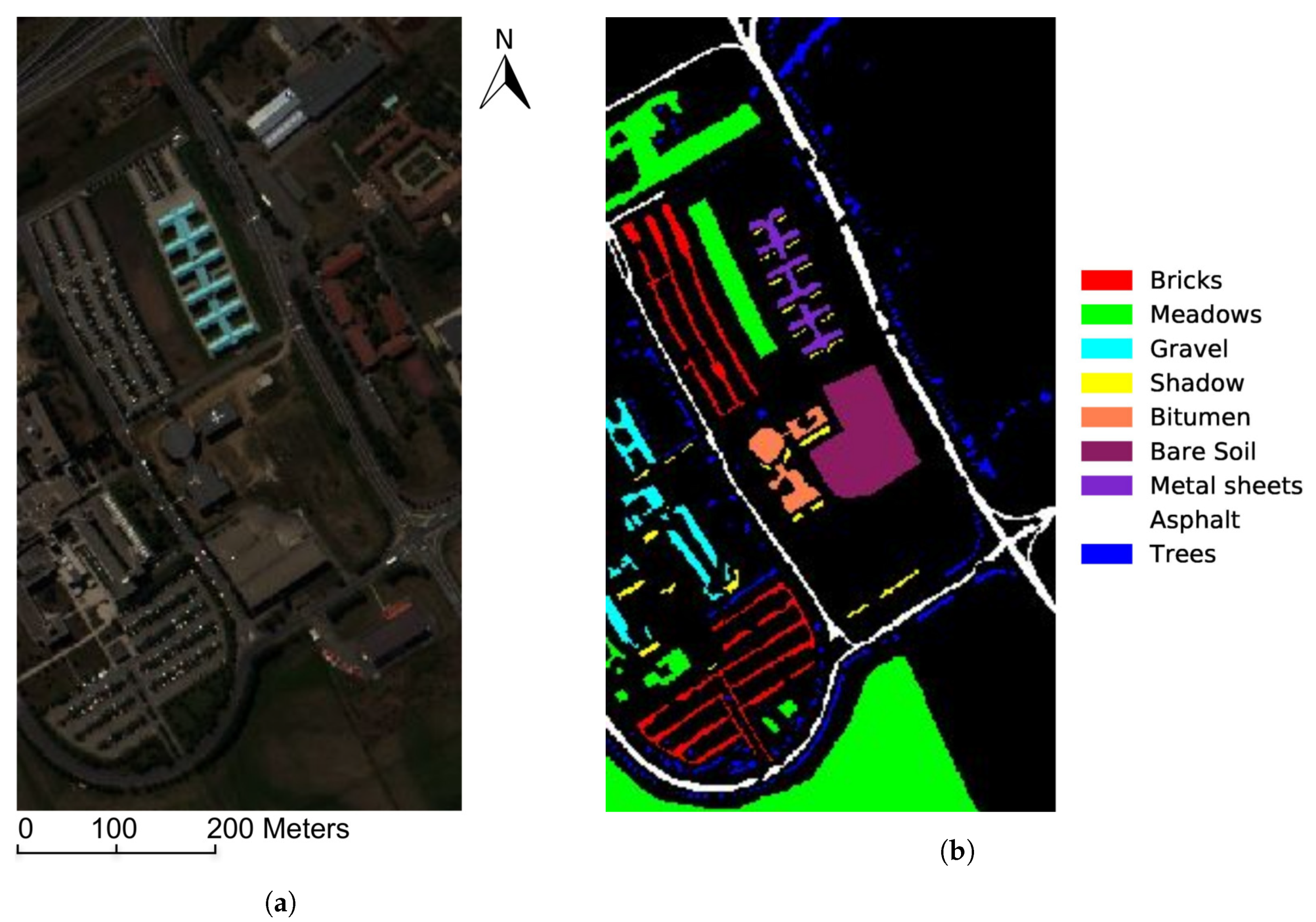
Figure 2.
Pavia University dataset. (a) false color composite image (bands 45, 27, and 11); (b) ground truth.
Figure 2.
Pavia University dataset. (a) false color composite image (bands 45, 27, and 11); (b) ground truth.
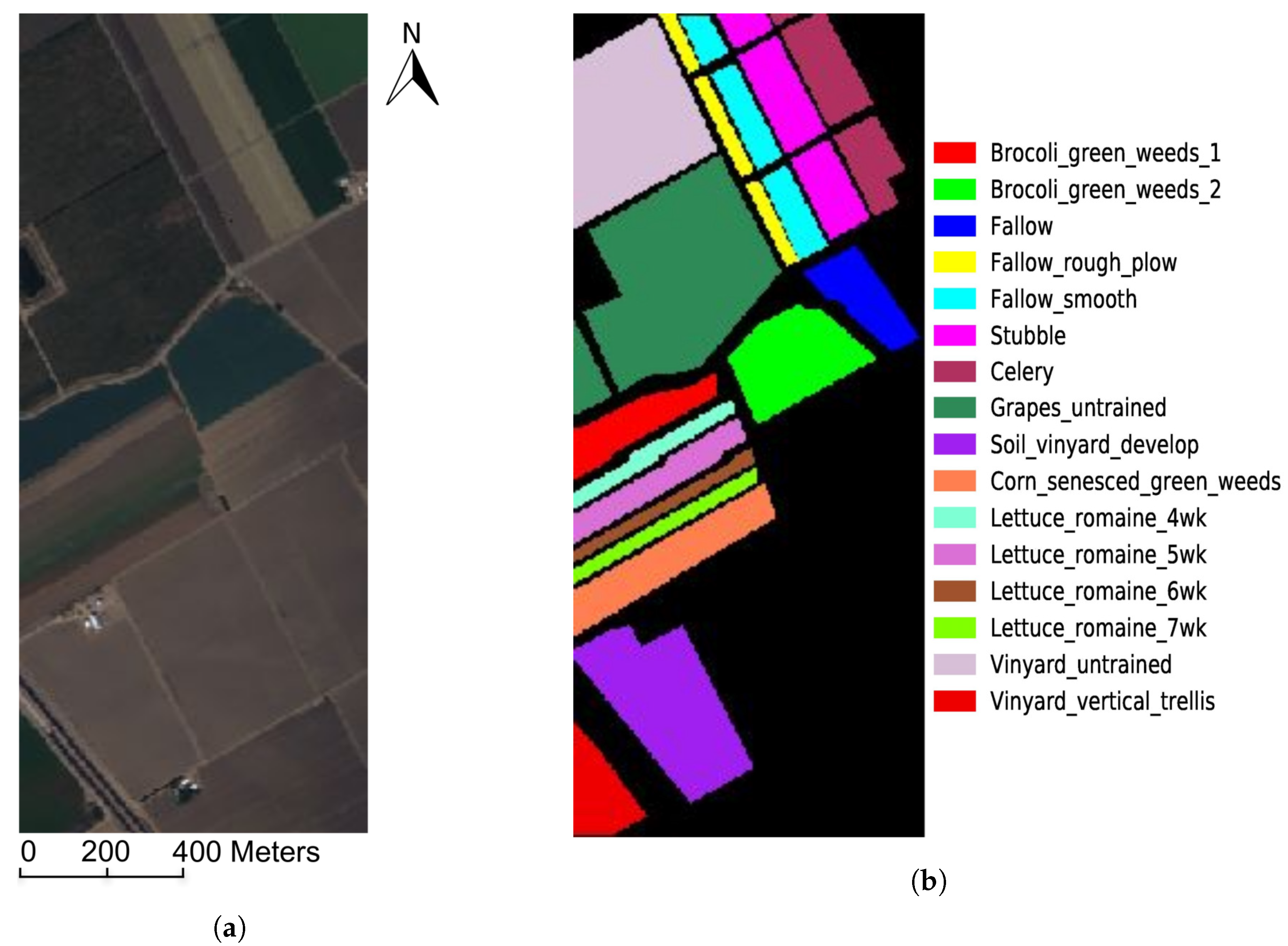
Figure 3.
Salinas dataset. (a) false color composite image (bands 29, 19, and 9); (b) ground truth.
Figure 3.
Salinas dataset. (a) false color composite image (bands 29, 19, and 9); (b) ground truth.
Figure 4.
Flevoland dataset.
Figure 4.
Flevoland dataset.
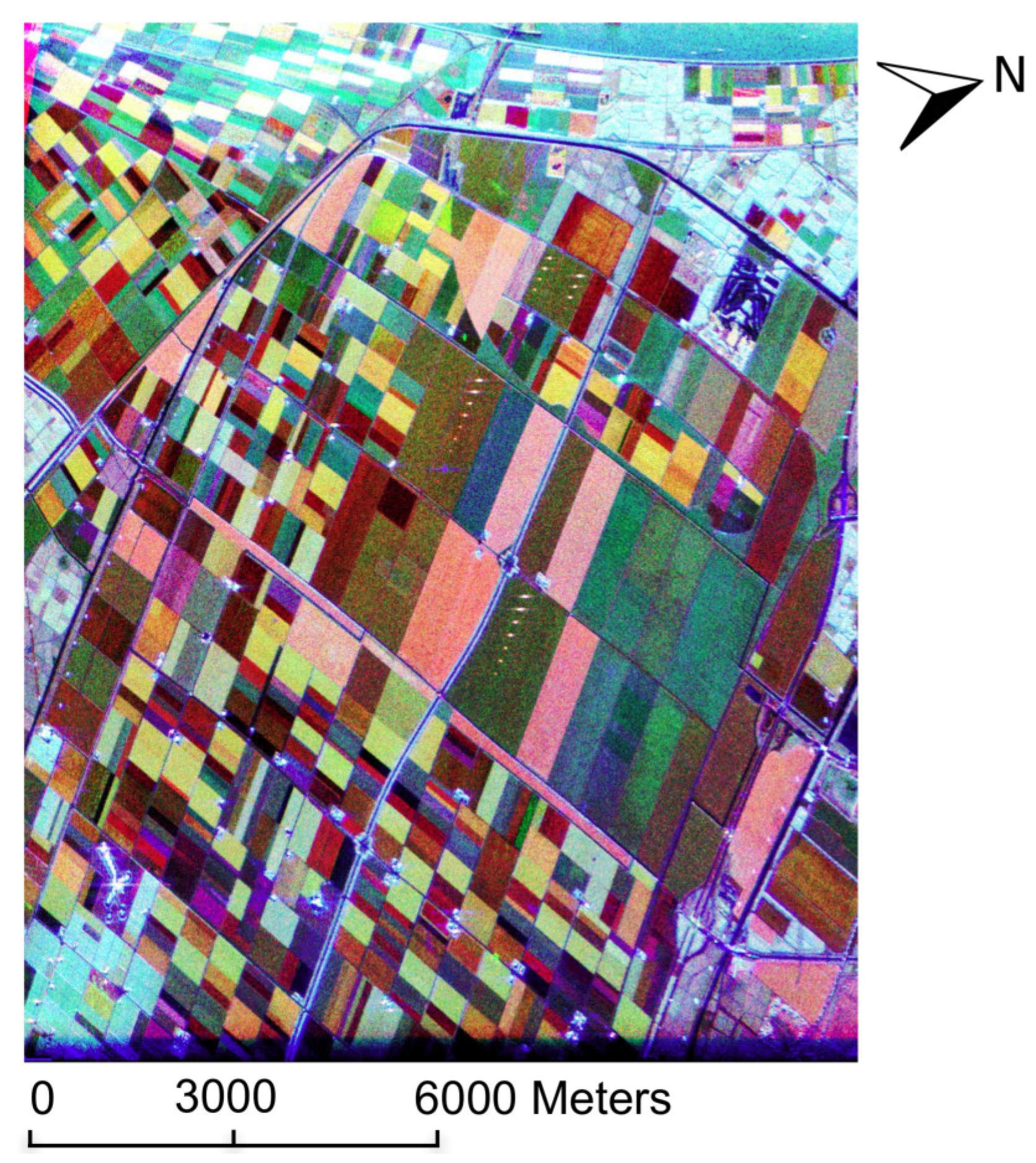
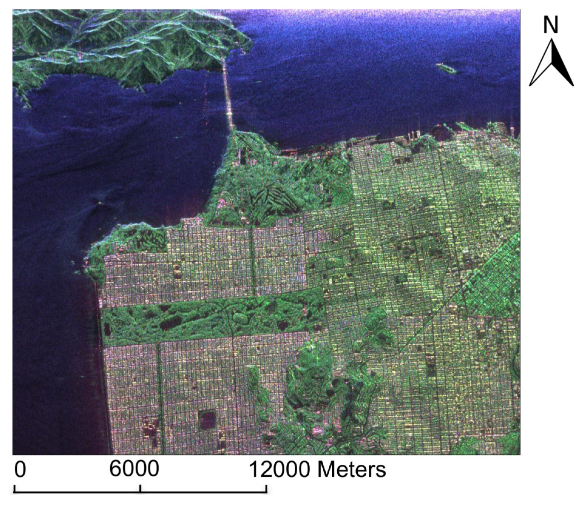
Figure 5.
San Francisco dataset.
Figure 5.
San Francisco dataset.
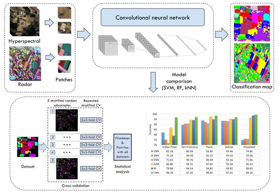
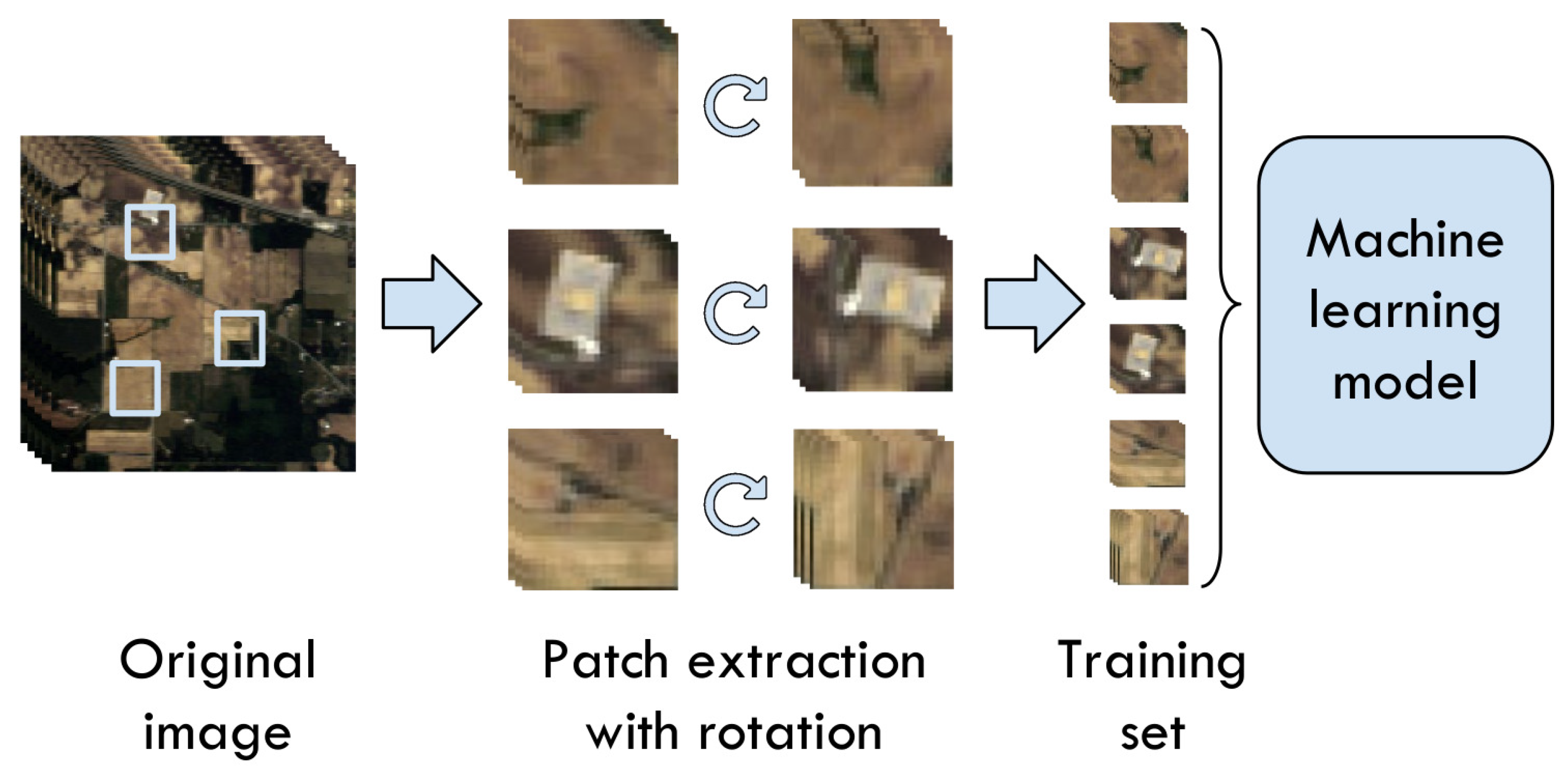
Figure 6.
Patch extraction process to generate the instances that would be fed to the ML models.
Figure 6.
Patch extraction process to generate the instances that would be fed to the ML models.
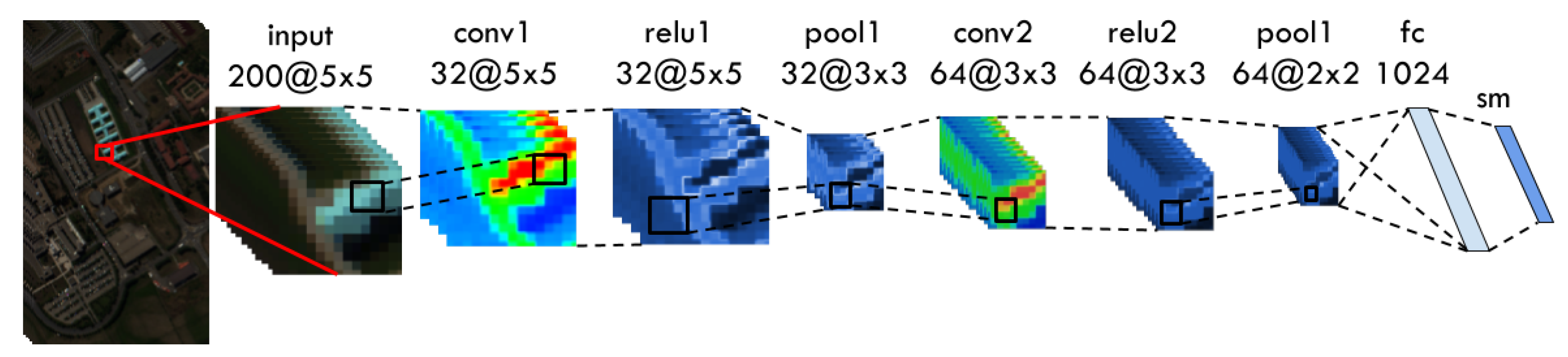
Figure 7.
CNN architecture. The conv layers refer to convolutional layers, pool to max-pooling layers, fc to the fully connected layer, and sm to the softmax layer. Dropout and batch normalization are omitted to simplify the visualization.
Figure 7.
CNN architecture. The conv layers refer to convolutional layers, pool to max-pooling layers, fc to the fully connected layer, and sm to the softmax layer. Dropout and batch normalization are omitted to simplify the visualization.
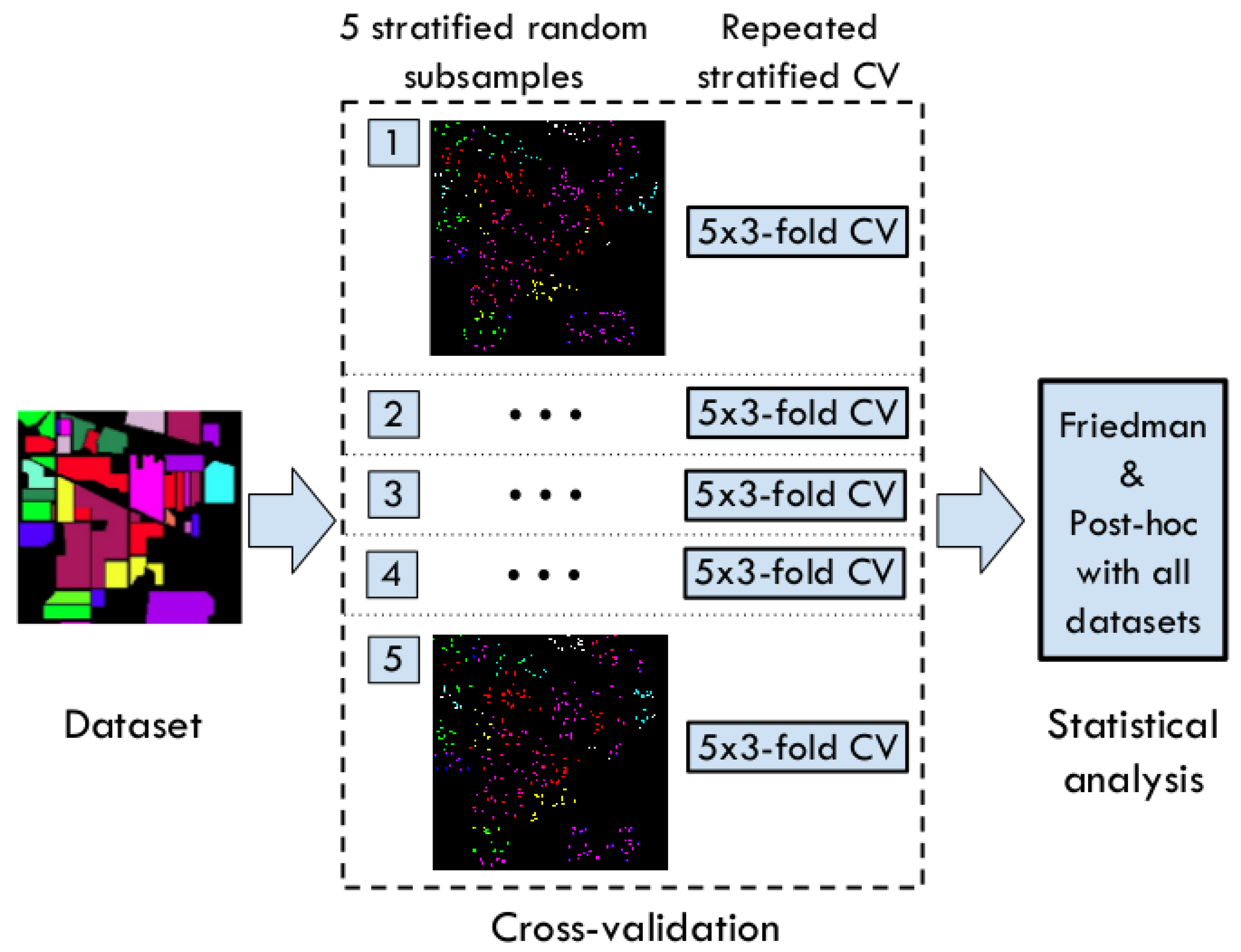
Figure 8.
Experimental setup. For each dataset, we obtain five independent subsamples and perform repeated stratified cross-validation. The collected results of all datasets are analyzed with a statistical test (Friedman and Post-hoc).
Figure 8.
Experimental setup. For each dataset, we obtain five independent subsamples and perform repeated stratified cross-validation. The collected results of all datasets are analyzed with a statistical test (Friedman and Post-hoc).
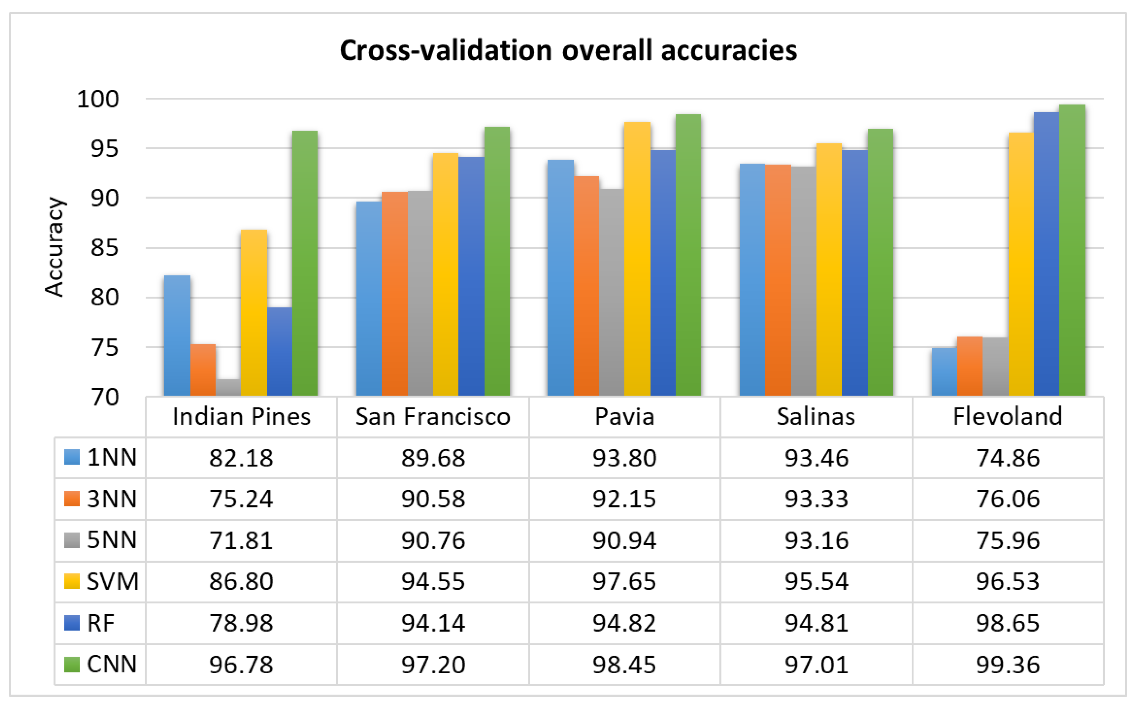
Figure 9.
Cross-validation overall accuracy of all methods over each dataset, ordered by increasing size of training set.
Figure 9.
Cross-validation overall accuracy of all methods over each dataset, ordered by increasing size of training set.
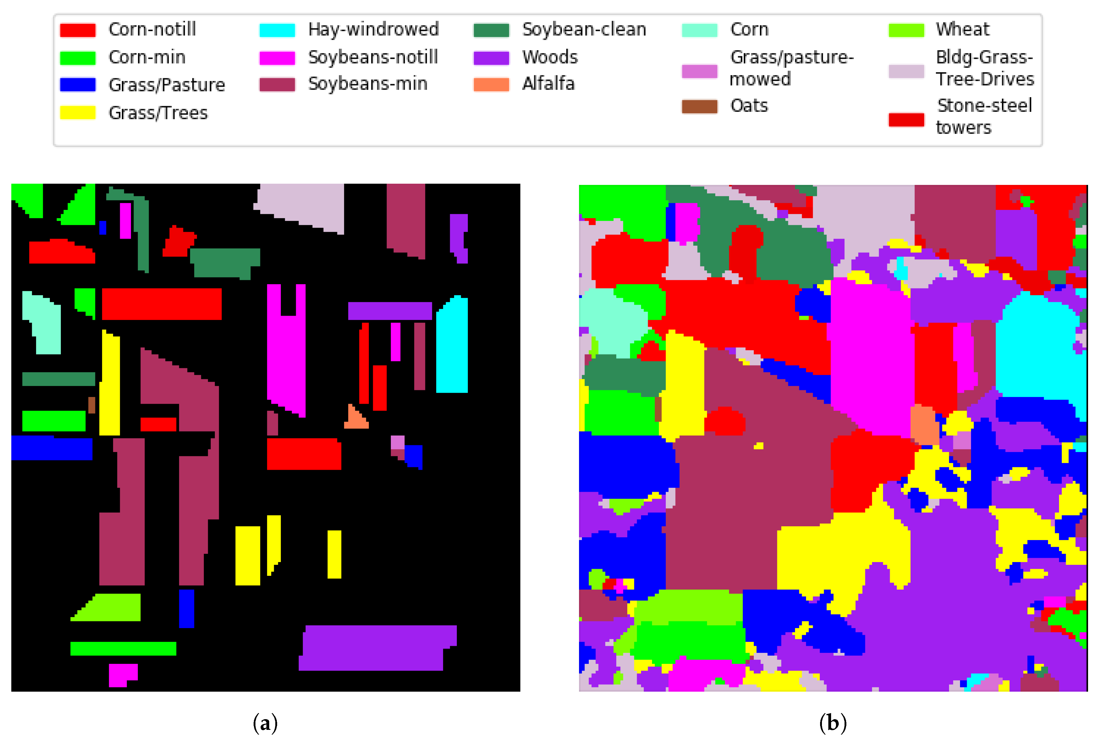
Figure 10.
Indian Pines GRSS competition. (a) training set; (b) classification map .
Figure 10.
Indian Pines GRSS competition. (a) training set; (b) classification map .
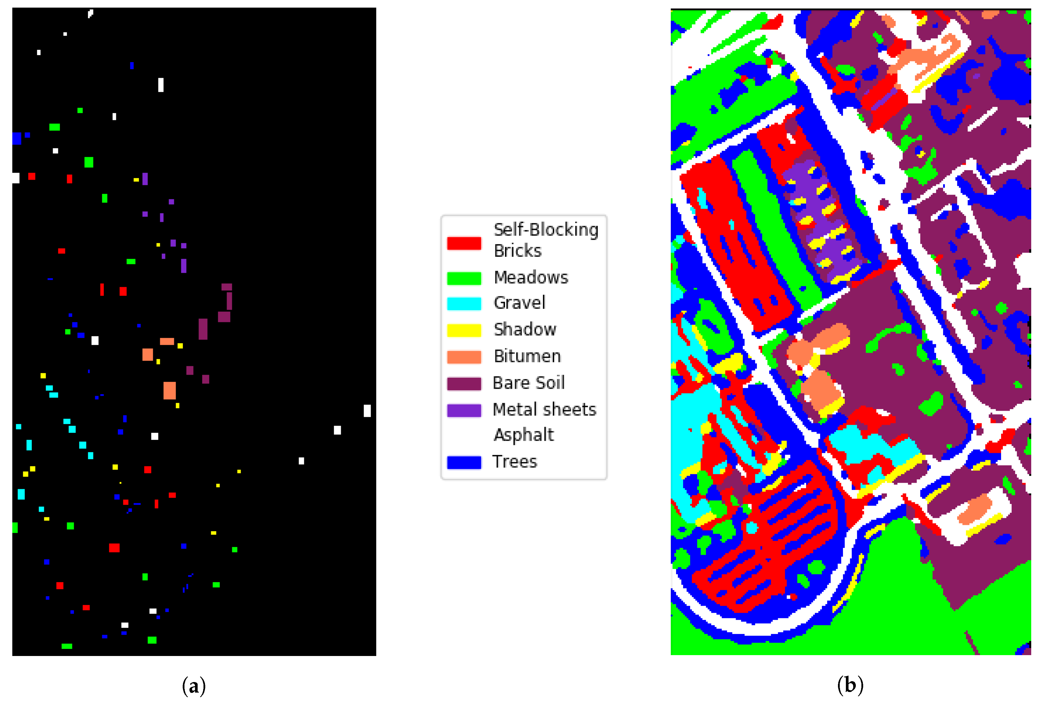
Figure 11.
Pavia University GRSS competition. (a) training set; (b) classification map .
Figure 11.
Pavia University GRSS competition. (a) training set; (b) classification map .
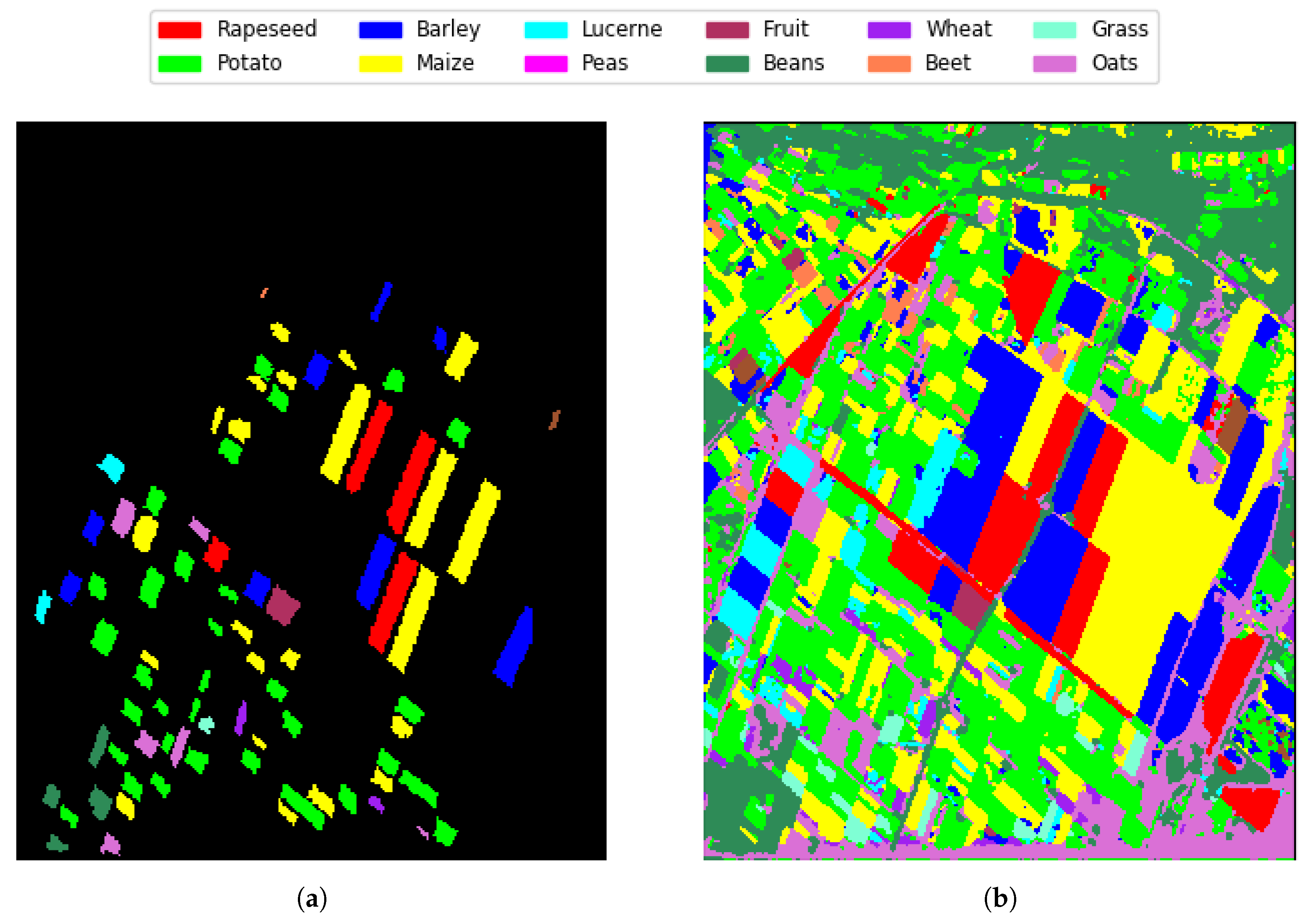
Figure 12.
Flevoland GRSS competition. (a) training set; (b) classification map .
Figure 12.
Flevoland GRSS competition. (a) training set; (b) classification map .
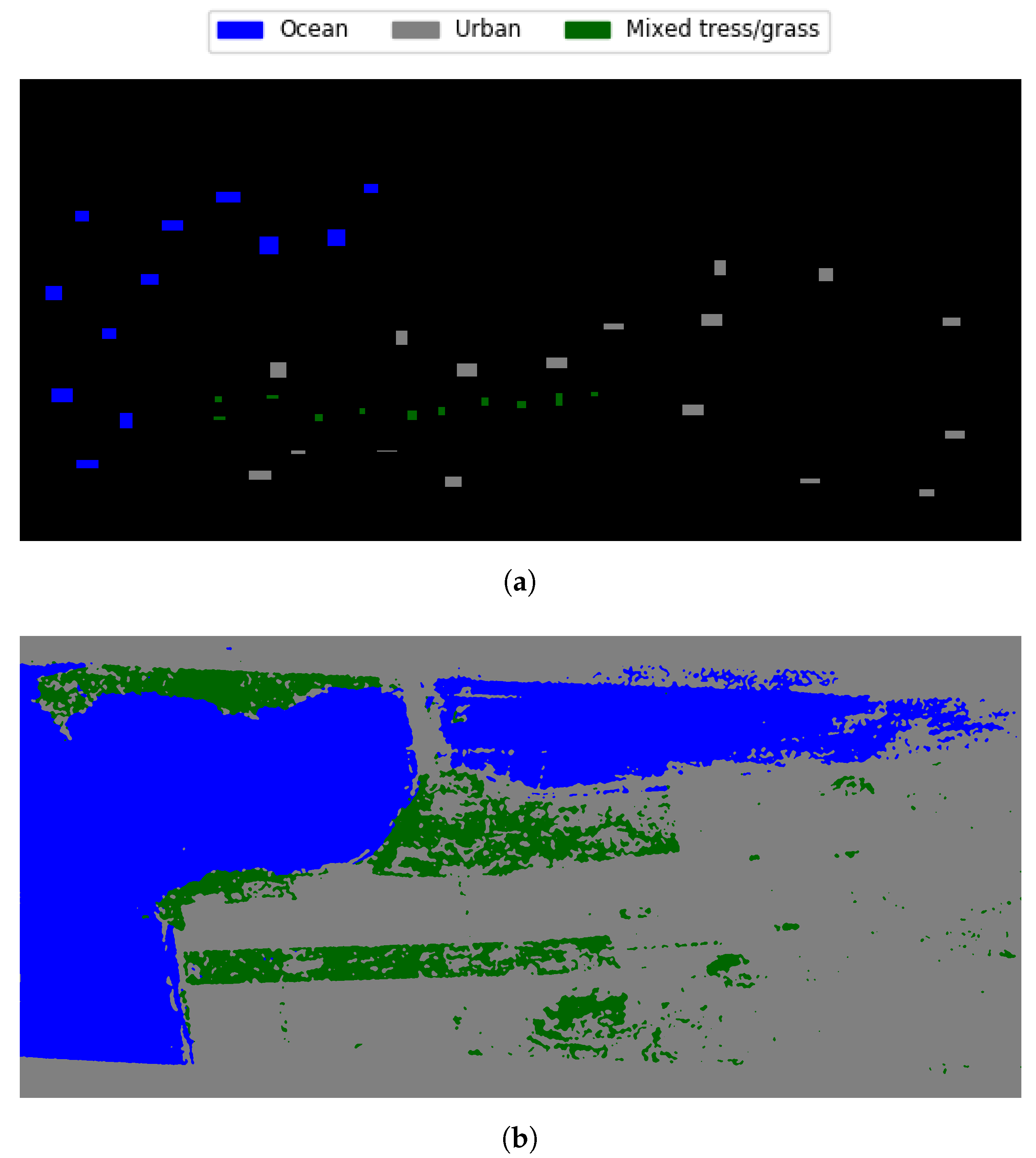
Figure 13.
San Francisco GRSS competition. (a) training set; (b) classification map .
Figure 13.
San Francisco GRSS competition. (a) training set; (b) classification map .
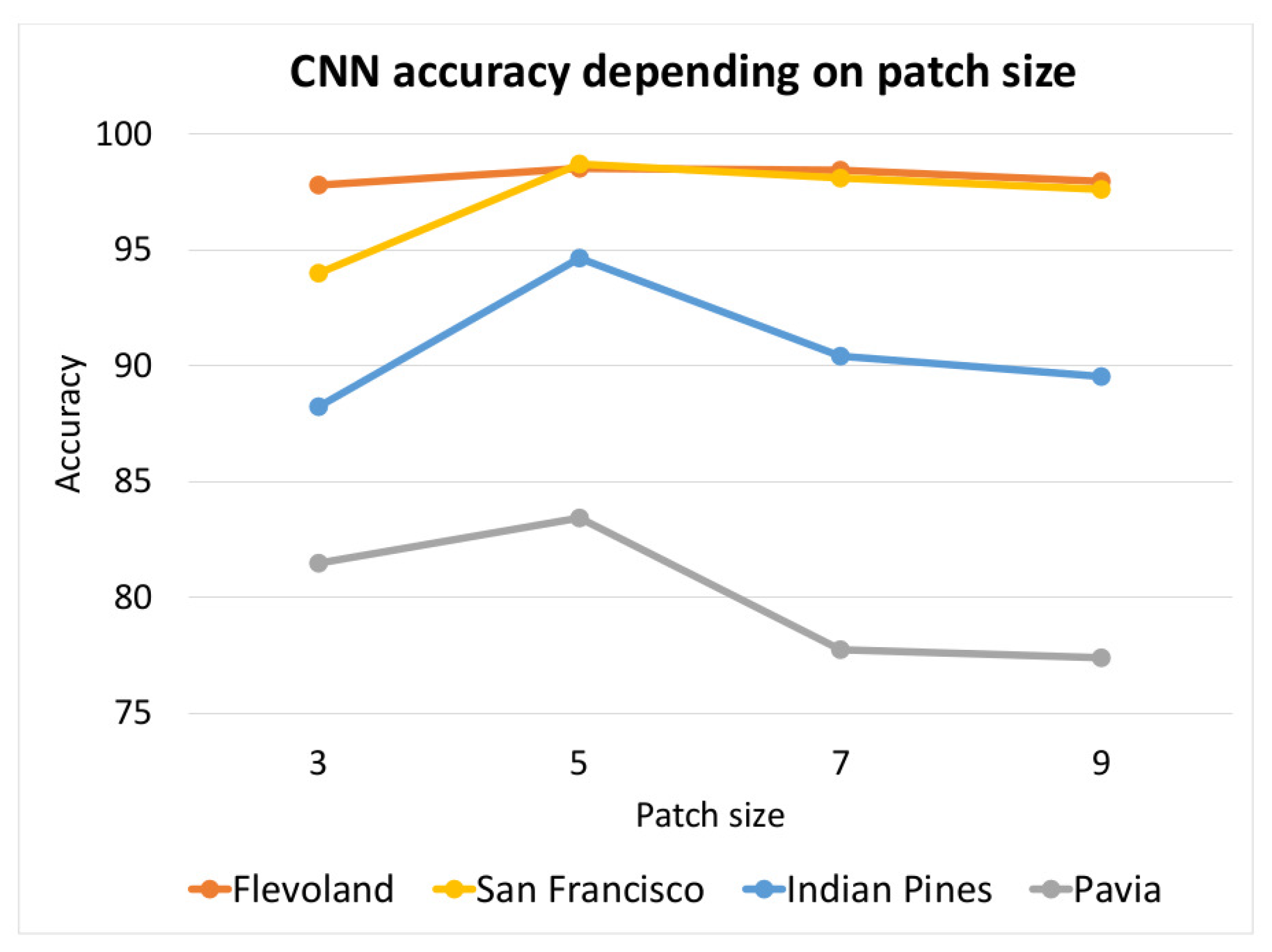
Figure 14.
Influence of patch size on classification accuracy over four datasets.
Figure 14.
Influence of patch size on classification accuracy over four datasets.
Table 1.
Description of datasets.
Table 1.
Description of datasets.
| Dataset | Type (Sensor) | Size | # Bands | Spatial Resolution | # Classes |
|---|
| Indian Pines | Hyperspectral (AVIRIS) | 145 × 145 | 220 | 20 m | 16 |
| Salinas | Hyperspectral (AVIRIS) | 512 × 217 | 204 | 3.7 m | 16 |
| Pavia | Hyperspectral (ROSIS) | 610 × 340 | 103 | 1.3 m | 9 |
| San Francisco | Radar (AirSAR) | 1168 × 2531 | 27 (P, L & C) | 10 m | 3 |
| Flevoland | Radar (AirSAR) | 1279 × 1274 | 27 (P, L & C) | 10 m | 12 |
Table 2.
CNN architecture. P refers to the input patch size (5 in our case), N to the number of channels of the input image, and C to the number of classes to consider.
Table 2.
CNN architecture. P refers to the input patch size (5 in our case), N to the number of channels of the input image, and C to the number of classes to consider.
| CNN Architecture |
|---|
| Layer | Type | Neurons & # Maps | Kernel |
|---|
| 0 | Input | | |
| 1 | Batch normalization | | |
| 2 | Convolutional | | |
| 3 | ReLU | | |
| 4 | Batch normalization | | |
| 5 | Max-Pooling | | |
| 6 | Convolutional | | |
| 7 | ReLU | | |
| 8 | Batch normalization | | |
| 9 | Max-Pooling | | |
| 10 | Fully connected | 1024 neurons | |
| 11 | Dropout | 1024 neurons | |
| 12 | Softmax | C neurons | |
Table 3.
Grid search and selected values for the training parameters of the CNN.
Table 3.
Grid search and selected values for the training parameters of the CNN.
| CNN Parameter Selection |
|---|
| Parameter | Grid Search | Selected Value |
|---|
| Dropout rate | {0.2, 0.5} | 0.2 |
| Learning rate | {0.1, 0.01, 0.001} | 0.01 |
| Decaying learning rate | {True, False} | True |
| Number of epochs | {20, 50, 80, 100} | 50 |
| Batch size | {16, 32, 64, 128} | 16 |
Table 4.
Indian Pines cross-validation results. Sample distribution in each experiment and individual class, overall, and average accuracies of all methods. Best results are highlighted in bold.
Table 4.
Indian Pines cross-validation results. Sample distribution in each experiment and individual class, overall, and average accuracies of all methods. Best results are highlighted in bold.
| Indian Pines Cross-Validation |
|---|
| Sample Distribution | Accuracy |
|---|
| # | Class | Samples | | 1NN | 3NN | 5NN | SVM | RF | CNN |
|---|
| 1 | Corn-notill | 286 | | 76.19 | 72.26 | 66.08 | 81.75 | 68.21 | 95.78 |
| 2 | Corn-min | 166 | | 69.28 | 59.02 | 54.05 | 74.60 | 62.03 | 93.32 |
| 3 | Grass/Pasture | 97 | | 93.83 | 91.35 | 88.38 | 92.59 | 88.45 | 96.56 |
| 4 | Grass/Trees | 146 | | 98.33 | 97.36 | 97.20 | 97.94 | 98.79 | 99.54 |
| 5 | Hay-windrowed | 96 | | 99.37 | 99.24 | 99.16 | 99.20 | 99.58 | 99.92 |
| 6 | Soybeans-notill | 195 | | 86.97 | 79.54 | 77.69 | 81.71 | 67.21 | 95.33 |
| 7 | Soybeans-min | 491 | | 86.83 | 81.21 | 79.79 | 92.40 | 91.40 | 97.22 |
| 8 | Soybean-clean | 119 | | 64.02 | 42.03 | 32.77 | 72.99 | 46.53 | 96.70 |
| 9 | Woods | 253 | | 89.23 | 86.46 | 85.50 | 97.00 | 95.99 | 98.46 |
| 10 | Alfalfa | 10 | | 62.67 | 35.89 | 13.44 | 31.89 | 25.22 | 94.22 |
| 11 | Corn | 48 | | 48.05 | 22.18 | 14.25 | 61.40 | 32.34 | 95.35 |
| 12 | Grass/pasture-mowed | 6 | | 70.00 | 51.33 | 26.00 | 35.33 | 11.33 | 94.67 |
| 13 | Oats | 4 | | 69.33 | 31.33 | 10.67 | 44.67 | 22.00 | 76.02 |
| 14 | Wheat | 41 | | 98.61 | 97.13 | 95.39 | 98.40 | 97.63 | 99.90 |
| 15 | Bldg-Grass-Tree-Drives | 78 | | 42.43 | 23.78 | 14.09 | 73.35 | 58.25 | 94.75 |
| 16 | Stone-steel towers | 19 | | 93.27 | 79.05 | 74.16 | 95.14 | 79.81 | 99.59 |
| | Total | 2055 | OA | 82.18 | 75.24 | 71.81 | 86.80 | 78.98 | 96.78 |
| | | | AA | 78.03 | 65.57 | 58.04 | 76.90 | 65.30 | 95.78 |
Table 5.
Pavia University cross-validation results. Sample distribution in each experiment and individual class, overall, and average accuracies of all methods. Best results are highlighted in bold.
Table 5.
Pavia University cross-validation results. Sample distribution in each experiment and individual class, overall, and average accuracies of all methods. Best results are highlighted in bold.
| Pavia University Cross-Validation |
|---|
| Sample Distribution | Accuracy |
|---|
| # | Class | Samples | | 1NN | 3NN | 5NN | SVM | RF | CNN |
|---|
| 1 | Self-Blocking Bricks | 737 | | 92.48 | 92.09 | 91.47 | 97.72 | 95.62 | 96.14 |
| 2 | Meadows | 3730 | | 99.18 | 99.43 | 99.52 | 99.85 | 98.83 | 99.97 |
| 3 | Gravel | 420 | | 87.62 | 85.18 | 83.52 | 88.67 | 81.71 | 91.25 |
| 4 | Shadow | 190 | | 99.85 | 99.79 | 99.83 | 99.87 | 100 | 99.64 |
| 5 | Bitumen | 266 | | 92.60 | 91.47 | 90.92 | 90.03 | 87.67 | 93.43 |
| 6 | Bare Soil | 1006 | | 75.67 | 66.28 | 59.89 | 95.65 | 79.80 | 99.14 |
| 7 | Metal sheets | 269 | | 100 | 100 | 100 | 100 | 99.66 | 100 |
| 8 | Asphalt | 1327 | | 95.21 | 93.75 | 92.69 | 96.33 | 97.96 | 98.24 |
| 9 | Trees | 613 | | 89.45 | 86.19 | 83.52 | 97.92 | 95.68 | 98.56 |
| | Total | 8558 | OA | 93.80 | 92.15 | 90.94 | 97.65 | 94.82 | 98.45 |
| | | | AA | 92.45 | 90.46 | 89.04 | 96.26 | 92.99 | 97.35 |
Table 6.
Salinas cross-validation results. Sample distribution in each experiment and individual class, overall, and average accuracies of all methods. Best results are highlighted in bold.
Table 6.
Salinas cross-validation results. Sample distribution in each experiment and individual class, overall, and average accuracies of all methods. Best results are highlighted in bold.
| Salinas Cross-Validation |
|---|
| Sample Distribution | Accuracy |
|---|
| # | Class | Samples | | 1NN | 3NN | 5NN | SVM | RF | CNN |
|---|
| 1 | Brocoli_green_weeds_1 | 402 | | 99.26 | 98.94 | 98.75 | 99.84 | 99.99 | 99.99 |
| 2 | Brocoli_green_weeds_2 | 746 | | 99.63 | 99.53 | 99.36 | 99.90 | 100 | 99.28 |
| 3 | Fallow | 396 | | 99.72 | 99.74 | 99.77 | 99.86 | 99.36 | 99.59 |
| 4 | Fallow_rough_plow | 279 | | 99.76 | 99.66 | 99.58 | 99.76 | 99.83 | 99.44 |
| 5 | Fallow_smooth | 536 | | 98.99 | 98.81 | 98.48 | 99.76 | 99.42 | 98.48 |
| 6 | Stubble | 792 | | 100 | 100 | 100 | 100 | 100 | 100 |
| 7 | Celery | 716 | | 99.90 | 99.83 | 99.77 | 99.94 | 99.97 | 99.95 |
| 8 | Grapes_untrained | 2255 | | 82.64 | 83.15 | 83.31 | 92.16 | 91.43 | 92.81 |
| 9 | Soil_vinyard_develop | 1241 | | 99.77 | 99.51 | 99.23 | 99.93 | 99.91 | 99.91 |
| 10 | Corn_green_weeds | 656 | | 97.08 | 95.48 | 94.41 | 98.70 | 97.62 | 98.47 |
| 11 | Lettuce_romaine_4wk | 214 | | 99.23 | 98.37 | 98.03 | 99.03 | 98.95 | 99.44 |
| 12 | Lettuce_romaine_5wk | 386 | | 100 | 99.98 | 100 | 100 | 100 | 100 |
| 13 | Lettuce_romaine_6wk | 184 | | 99.98 | 100 | 100 | 99.98 | 99.96 | 99.52 |
| 14 | Lettuce_romaine_7wk | 214 | | 98.43 | 97.44 | 96.96 | 99.24 | 97.70 | 99.20 |
| 15 | Vinyard_untrained | 1454 | | 81.28 | 81.15 | 80.84 | 80.34 | 77.01 | 91.34 |
| 16 | Vinyard_vertical_trellis | 362 | | 98.94 | 98.29 | 97.90 | 99.26 | 98.90 | 99.58 |
| | Total | 10833 | OA | 93.46 | 93.33 | 93.16 | 95.54 | 94.81 | 97.03 |
| | | | AA | 97.16 | 96.87 | 96.65 | 97.98 | 97.50 | 98.56 |
Table 7.
San Francisco cross-validation results. Sample distribution in each experiment and individual class, overall, and average accuracies of all methods. Best results are highlighted in bold.
Table 7.
San Francisco cross-validation results. Sample distribution in each experiment and individual class, overall, and average accuracies of all methods. Best results are highlighted in bold.
| San Francisco Cross-Validation |
|---|
| Sample Distribution | Accuracy |
|---|
| # | Class | Samples | | 1NN | 3NN | 5NN | SVM | RF | CNN |
|---|
| 1 | Ocean | 3383 | | 100 | 100 | 100 | 100 | 100 | 100 |
| 2 | Urban | 3594 | | 91.50 | 94.92 | 96.04 | 94.27 | 99.38 | 96.97 |
| 3 | Mixed trees/grass | 770 | | 35.83 | 28.93 | 25.48 | 71.88 | 43.93 | 85.97 |
| | Total | 7747 | OA | 89.68 | 90.58 | 90.76 | 94.55 | 94.14 | 97.20 |
| | | | AA | 75.78 | 74.62 | 73.84 | 88.72 | 81.10 | 94.31 |
Table 8.
Flevoland cross-validation results. Sample distribution in each experiment and individual class, overall, and average accuracies of all methods. Best results are highlighted in bold.
Table 8.
Flevoland cross-validation results. Sample distribution in each experiment and individual class, overall, and average accuracies of all methods. Best results are highlighted in bold.
| Flevoland Cross-Validation |
|---|
| Sample Distribution | Accuracy |
|---|
| # | Class | Samples | | 1NN | 3NN | 5NN | SVM | RF | CNN |
|---|
| 1 | Rapeseed | 3525 | | 51.23 | 54.09 | 54.83 | 99.63 | 100 | 100 |
| 2 | Potato | 6571 | | 82.96 | 88.02 | 88.06 | 98.47 | 99.32 | 99.23 |
| 3 | Barley | 3295 | | 68.89 | 67.09 | 65.00 | 95.84 | 99.52 | 99.44 |
| 4 | Maize | 8004 | | 96.27 | 96.83 | 97.24 | 98.00 | 99.80 | 99.62 |
| 5 | Lucerne | 468 | | 12.20 | 6.10 | 6.56 | 96.29 | 86.55 | 98.73 |
| 6 | Peas | 482 | | 60.23 | 59.45 | 58.77 | 86.81 | 99.99 | 99.99 |
| 7 | Fruit | 832 | | 4.36 | 0.92 | 1.08 | 88.96 | 99.45 | 99.47 |
| 8 | Beans | 252 | | 18.30 | 7.63 | 7.98 | 82.15 | 93.29 | 95.02 |
| 9 | Wheat | 24 | | 50.50 | 27.83 | 17.01 | 6.83 | 13.33 | 77.33 |
| 10 | Beet | 112 | | 7.77 | 1.04 | 0.21 | 58.11 | 59.23 | 98.43 |
| 11 | Grass | 1160 | | 73.50 | 72.45 | 71.42 | 89.78 | 96.18 | 99.20 |
| 12 | Oats | 72 | | 36.00 | 24.78 | 20.78 | 36.89 | 12.72 | 74.39 |
| | Total | 24797 | OA | 74.86 | 76.06 | 75.96 | 96.53 | 98.65 | 99.36 |
| | | | AA | 46.85 | 42.19 | 40.74 | 78.15 | 79.95 | 95.06 |
Table 9.
Average computation time(s) of the cross-validation experiments for all datasets over different classifiers. The fastest methods are highlighted in bold.
Table 9.
Average computation time(s) of the cross-validation experiments for all datasets over different classifiers. The fastest methods are highlighted in bold.
| Computation Time (s) |
|---|
| | Training | Test |
|---|
| Dataset | SVM | RF | CNN CPU | CNN GPU | SVM | RF | CNN CPU | CNN GPU |
|---|
| Indian Pines | 90.2 | 36.4 | 84.2 | 16.1 | 15.1 | 0.11 | 0.05 | 0.03 |
| Pavia | 150.1 | 140.5 | 186.6 | 71.3 | 33.2 | 0.14 | 0.11 | 0.06 |
| Salinas | 294.1 | 153.4 | 272.3 | 82.1 | 96.9 | 0.31 | 0.24 | 0.15 |
| San Francisco | 24.8 | 23.9 | 95.2 | 49.6 | 4.8 | 0.12 | 0.06 | 0.05 |
| Flevoland | 826.4 | 234.1 | 313.6 | 160.8 | 89.1 | 0.42 | 0.21 | 0.17 |
Table 10.
Friedman test ranking.
Table 10.
Friedman test ranking.
| Friedman Test Ranking |
|---|
| CNN | 1.000 |
| SVM | 2.240 |
| RF | 2.960 |
| 1NN | 4.600 |
| 3NN | 4.840 |
| 5NN | 5.360 |
Table 11.
Holm’s post hoc analysis.
Table 11.
Holm’s post hoc analysis.
| Post Hoc Analysis |
|---|
| Method | p | z | Holm |
|---|
| 5NN | 0.0000 | 8.2396 | 0.0100 |
| 3NN | 0.0000 | 7.2569 | 0.0125 |
| 1NN | 0.0000 | 6.8034 | 0.0167 |
| RF | 0.0002 | 3.7041 | 0.0250 |
| SVM | 0.0191 | 2.3434 | 0.0500 |
Table 12.
Overall accuracies obtained for each method at the GRSS DASE Website competition.
Table 12.
Overall accuracies obtained for each method at the GRSS DASE Website competition.
| Accuracies GRSS DASE Website Competition |
|---|
| | 1NN | 3NN | 5NN | SVM | RF | CNN | CNN-MF |
|---|
| Indian Pines | 64.75 | 64.55 | 65.14 | 86.31 | 64.33 | 94.64 | 95.53 |
| San Francisco | 90.50 | 91.86 | 92.40 | 96.28 | 96.81 | 98.70 | 99.37 |
| Pavia | 63.85 | 62.60 | 62.78 | 79.75 | 65.02 | 83.43 | 84.79 |
| Flevoland | 78.55 | 78.96 | 77.54 | 95.51 | 96.22 | 98.51 | 99.05 |
Table 13.
Influence of input patch size of the CNN on classification accuracy with different images.
Table 13.
Influence of input patch size of the CNN on classification accuracy with different images.
| CNN Accuracy Depending on Patch Size |
|---|
| | 3 × 3 | 5 × 5 | 7 × 7 | 9 × 9 |
|---|
| Indian Pines | 88.23 | 94.64 | 90.41 | 89.53 |
| Pavia | 81.48 | 83.43 | 77.75 | 77.4 |
| Flevoland | 97.79 | 98.51 | 98.43 | 97.95 |
| San Francisco | 93.99 | 98.70 | 98.09 | 97.6 |


