Article

Strength in Numbers: Combining Multi-Source Remotely Sensed Data to Model Plant Invasions in Coastal Dune Ecosystems

1
Department of Applied Geoinformatics and Spatial Planning, Faculty of Environmental Sciences, Czech University of Life Sciences, Kamycka 129, 165 21 Prague 6, Czech Republic
2
CSIRO Land & Water, 147 Underwood Avenue, Floreat, WA 6014, Australia
3
Department of Sciences, Roma Tre University, Viale G. Marconi 446, 00146 Rome, Italy
4
Envix-Lab, Department of Biosciences and Territory, Molise University, Contrada Fonte Lappone, 86090 Pesche (IS), Italy
5
University of Rennes 1, UMR CNRS 6553 EcoBio, 263 Avenue du Gal Leclerc, CS 74205, 35042 Rennes CEDEX, France
*
Author to whom correspondence should be addressed.
Remote Sens. 2019, 11(3), 275; https://doi.org/10.3390/rs11030275
Submission received: 2 January 2019 / Revised: 27 January 2019 / Accepted: 28 January 2019 / Published: 30 January 2019

Abstract

:
A common feature of most theories of invasion ecology is that the extent and intensity of invasions is driven by a combination of drivers, which can be grouped into three main factors: propagule pressure (P), abiotic drivers (A) and biotic interactions (B). However, teasing apart the relative contribution of P, A and B on Invasive Alien Species (IAS) distributions is typically hampered by a lack of data. We focused on Mediterranean coastal dunes as a model system to test the ability of a combination of multi-source Remote Sensing (RS) data to characterize the distribution of five IAS. Using generalized linear models, we explored and ranked correlates of P, A and B derived from high-resolution optical imagery and three-dimensional (3D) topographic models obtained from LiDAR, along two coastal systems in Central Italy (Lazio and Molise Regions). Predictors from all three factors contributed significantly to explaining the presence of IAS, but their relative importance varied among the two Regions, supporting previous studies suggesting that invasion is a context-dependent process. The use of RS data allowed us to characterize the distribution of IAS across broad, regional scales and to identify coastal sectors that are most likely to be invaded in the future.

Graphical Abstract

1. Introduction

Invasive alien species (IAS) have become a global conservation issue, constituting a major threat to biodiversity and requiring costly management programs to control their spread [1,2,3]. Yet, successful invasions are relatively rare, with only around 1 in 10 introduced species becoming established and only 10% of these having a sizable impact on the communities they invade [4]. This suggests that in many cases the most effective solution to mitigating the impact of IAS lies in their early detection and rapid intervention [5]. Consequently, new approaches for understanding what drives the distribution of IAS across broad spatial scales are urgently needed.
Numerous hypotheses have been put forward to explain why a given species may (or may not) become invasive outside of its native range [6]. These hypotheses largely converge on the fact that the outcome of an invasion event is determined by a combination of environmental drivers and biotic interactions that are typically context dependent [7,8]. Catford et al. [7] proposed an integrative framework for predicting the extent and intensity of invasions based on a combination of drivers which can be grouped into three main factors: propagule pressure (P), abiotic drivers (A) and biotic interactions (B) (hereon PAB framework).
Species Distribution Models (SDMs) provide one way of testing the PAB framework for predicting the geographic distribution of IAS [9,10] as well as identifying potential invasion hotspots to help guide management [11,12]. However, teasing apart the relative contribution of different PAB drivers on IAS distributions at scales relevant for management and conservation is typically hampered by a lack of data. In this regard, remote sensing (RS) technologies provide a cost-effective way to circumvent this problem [13,14]. In recent decades, RS has boosted the performance of SDMs by providing access to new ecologically-meaningful predictors of species distributions derived from a wide range of spectral and structural imagery [15,16]. A critical next step is to combine these new data streams with ecological theory to improve our ability to predict where IAS are most likely to present a threat to native ecosystems [17].
Here, we focused on Mediterranean coastal dunes as a model system to test the ability of RS data to characterize the distribution of IAS across strong environmental and land-use gradients. Mediterranean coastal dune ecosystems harbor unique biodiversity and provide critical ecosystem services, but are increasingly threatened by a range of global change drivers, among which are IAS [18,19,20,21]. Using a combination of multi-source RS data–including high-resolution optical imagery and three-dimensional (3D) topographic models obtained from LiDAR (Light Detection and Ranging)–we aimed to derive robust correlates of P, A and B at landscape scales. By combining these with a comprehensive spatial database capturing the occurrence of invasive plant species in coastal dune ecosystems of central Italy, we then tested the effectiveness of the PAB framework for predicting the distribution of IAS across these ecosystems and identifying potential invasion hotspots in the region. In addition, we quantified and ranked the relative impact of each PAB component affecting invasion outcome.

2. Materials and Methods
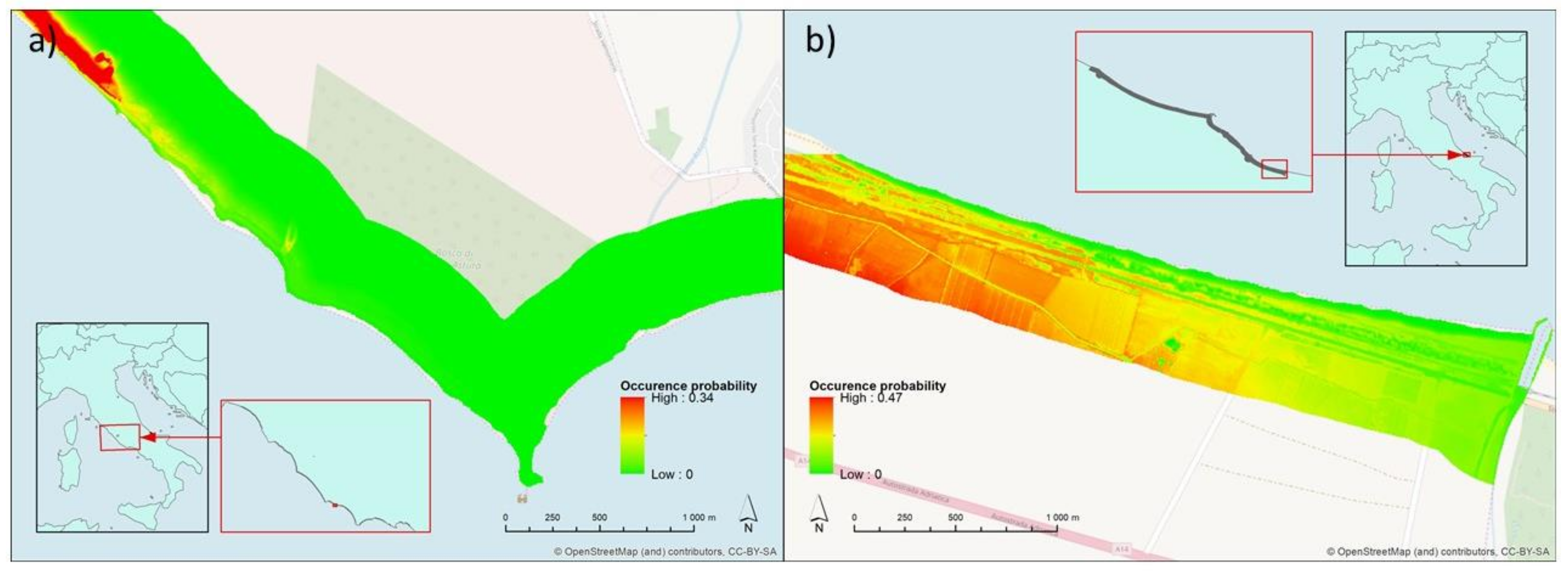
2.1. Study Area

The study was carried out on representative tracts of recent (Holocenic) coastal dunes of the Tyrrhenian (Lazio) and Adriatic coast (Molise) in Central Italy. The study area stretches for 90 km of coastlines in Lazio and 30 km in Molise. Both areas are characterized by a Mediterranean bioclimate that on the Adriatic side gives way to a temperate zone in the north [22]. In Central Italy, coastal dunes occupy a narrow strip along the seashore and are usually less than 8–10 m in height. Under natural conditions vegetation is naturally distributed along a zonation which follows the sea-inland ecological gradient [23,24], ranging from pioneer annual communities on the upper beach to Mediterranean maquis on inland fixed dunes. However, as has happened in many Mediterranean coastal systems [20], human-related disturbances (e.g., urbanization, tourism) have severely modified these coastal ecosystems [25,26]. For this reason, the vegetation sampled in our study area can be considered representative of the typical zonation found in most remaining Mediterranean coastal dunes.

2.2. Invasive Species Data

Field records detailing the location of invasive plant species along the coastlines of Lazio and Molise were derived from an existing database of vegetation plots “Ranvegdunes” [27]. Plots were 8 × 8 m in size (64 m2) and were established at the beginning of the growing season (April–May) between 2002 and 2011. The location of each plot was assigned randomly and subsequently recorded using a GPS to within 3 m accuracy. The presence of all vascular plant species (including IAS) was recorded in each plot. Following Acosta et al. [28] and Celesti-Grapow et al. [29], a total of five IAS were identified across the plot network. Of these, three were found along the Thyrrenian coast in Lazio (Agave americana, Carpobrotus acinaciformis, Carpobrotus edulis) and two along the Adriatic coast in Molise (Erigeron canadensis L., Oenothera stucchii Soldano) (for information about presence records for each IAS see Table S1). Note that here we define IAS as a subset of introduced plants that produce reproductive offspring (often in very large numbers) at considerable distances from the parent plants, and thus have the potential to spread over a large area [30].
These five IAS are characterized by different ecological strategies (annual or perennial evergreen strategies), origin (North/Central America and South Africa), introduction pathway (gardens or agricultural escapes) and impact on the invaded environment. Previous work has highlighted the impacts of Carpobrotus spp. and Agave americana invasions on ecosystem functioning and diversity in coastal ecosystems [31,32]. By contrast, Erigeron canadensis L. has been associated with a reduction in soil fertility and a decline of agricultural yields [33,34].

2.3. Remotely Sensed Data

Two high-resolution land-cover maps of the coasts of Lazio and Molise were derived from 1 m resolution panchromatic aerial orthophotos acquired in 2008 (accessible on the WMS of the Geoportale nazionale, http://www.pcn.minambiente.it/mattm/) covering a 500 m wide strip starting from the seashore [35,36]. Specifically, 10 land cover types were visually interpreted and mapped in a GIS environment [37] (ArcGIS 10.1, Environmental Systems Research Institute, Redlands, CA, USA) following the European standard CORINE land cover (CLC) classes expanded to a fourth level of detail for natural and semi-natural areas (Table S2). The accuracy of the land cover map was assessed by comparing the attribution of each class in the map with the data obtained through field surveys (performed in 2012 and 2013). The global accuracy of the maps calculated using the KHAT statistic was 0.77 [38]. The land cover map was converted to a raster grid with 5 m resolution from which we derived a set of variables that were used as surrogates of P and B in later analyses (described below; [9]). In addition to the land cover maps, a 2 m resolution digital terrain model (DTM) for both study regions, obtained from Airborne LiDAR imagery and acquired in the context of the Piano Straordinario di Telerilevamento Ambientale (Ministero dell’Ambiente e della Tutela del Territorio e del Mare) in 2008, was used to derive surrogates for field-measured environmental variables [39]. From the DTM, we calculated a set of topographic variables designed to reflect abiotic conditions (A) along the sea-inland environmental gradient [24].

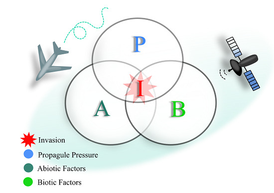
2.4. Mapping of Propagule Pressure, Abiotic Conditions and Biotic Environment

For each vegetation plot, three sets of proxy variables representing PAB factors that we hypothesized to influence plant invasions in coastal areas were obtained from the remotely sensed data described above (Table 1) [9].
As proxies of P, we calculated the proportion (%) of artificial (ART) and agricultural (AGR) land [39,40] as well as the distance from the nearest major road [12]. The ART and AGR were derived from the rasterized land cover maps by means of a moving window (50 m radius) algorithm implemented in R (R Foundation for Statistical Computing, Vienna, Austria). Previous work identified a 50 m radius window as adequate for analyzing coastal dune ecosystems at landscape scales [40]. Distance from major roads was calculated by measuring the straight line Euclidean distance of each plot from the closest highway or primary road (road data retrieved from https://planet.openstreetmap.org/; OpenStreetMap contributors, 2016, St John’s Innovation Centre, Cambridge, UK).
As proxies of A, dune elevation (m.a.s.l.) and slope (degrees) were derived from the DTM. These two topographic features relate directly to the sea-inland environmental gradient that is known to shape plant communities in these ecosystems [9,24,41]. In addition to this, for each plot we calculated the distance from the shoreline (derived from the land cover map) as a descriptor of A.
To capture B, we calculated the proportion (%) of the following natural and semi-natural land cover categories occurring in proximity of each plot [9,42]: afforestation (AFF), semi-natural herbaceous and woody dune vegetation (SN), wetland and marshes (WET), beach with pioneer annual vegetation (BPV), herbaceous dune vegetation (HDV) and woody dune vegetation (WDV) (see Table S2). The percentage of natural and semi-natural land cover types was derived from the rasterized land cover maps by means of a moving window (50 m radius) procedure implemented in R.

2.5. Species Distribution Modelling
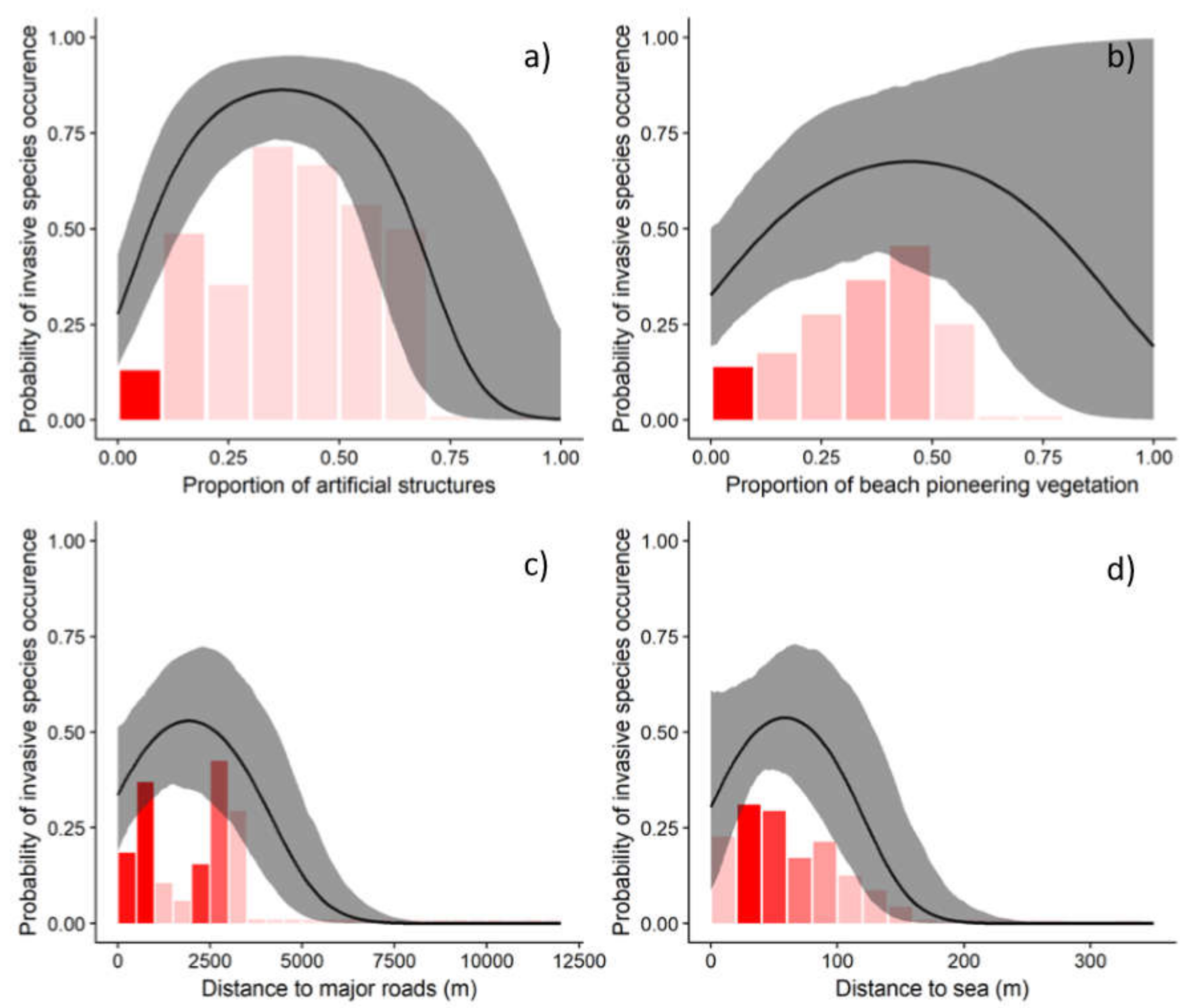
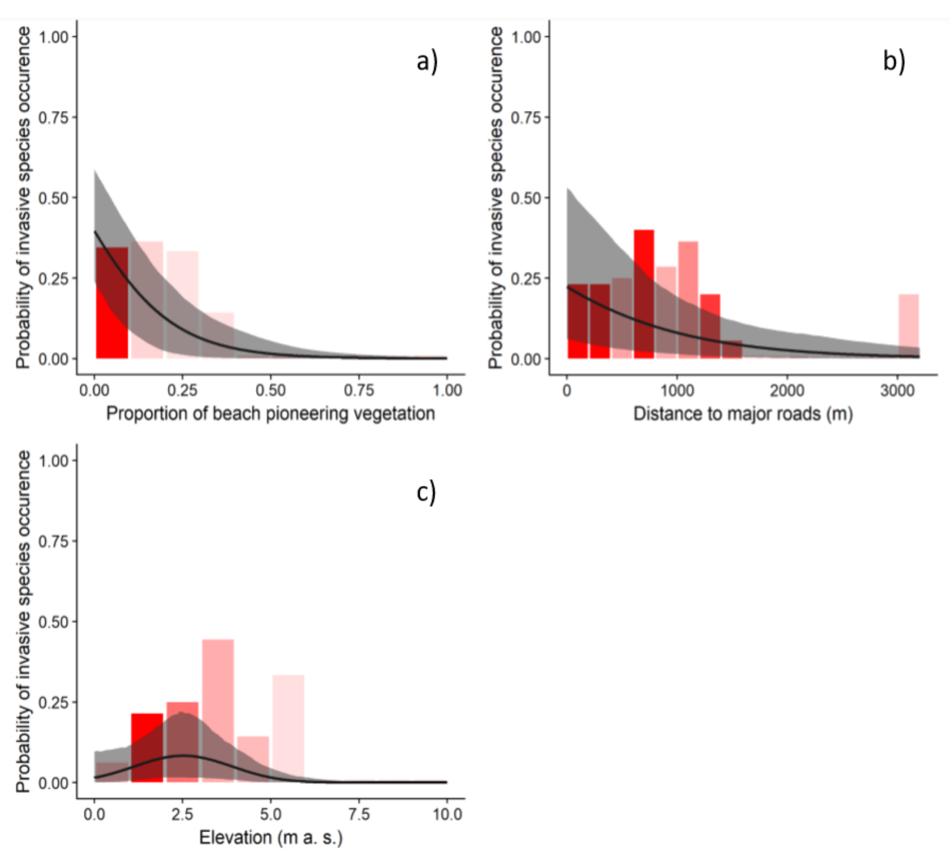
We modeled the occurrence of the five IAS using a binomial generalized linear model (GLM) with logit link function using the PAB variables described above (and listed in Table 1) as model predictors. In particular, PAB values for presences were extrapolated from plots were at least one of the IAS was recorded, while, at the same time, PAB values for absences from plots where any IAS was recorded. As we expected different predictors to shape the distribution of the IAS along the coasts of Lazio and Molise (due to inherent ecological differences among the species, as well as differences in the environmental and anthropogenic context of the two coastlines), we grouped the species from each of the two regions and analyzed them separately.
In a first step, a visual inspection of the data was used to explore how the presence/absence of IAS varied in response to each of the predictor variables. Based on this, we chose to include quadratic terms for predictors, which exhibited non-linear relationships with IAS occurrence (see Table 2 for details). In addition, we converted all land cover predictors for which ≥ 80 % of plots had a zero value from proportions (%) to presence/absence. To avoid issues with multicollinearity (e.g., due to strong correlations between the proportions of different land cover classes); then, we used variance inflection factors (VIF) to identify strongly correlated predictors (VIF > 5). As a result, we excluded WDV (VIF = 18.7) and AFF (VIF = 12.8) from the models fitted to the data from Lazio and Molise, respectively.
The full models for each of the two regions are presented in Table 2. Using these as starting points, we used backward model selection based on the Aikake Information Criterion (AIC) to identify the most parsimonious model for each of the two regions (function stepAIC in the MASS R package) [43]. Furthermore, we evaluated the contribution of predictors capturing each of the three domains (P, A and B) by comparing the model with and without all the predictors belonging to each domain based on changes in residual deviance.

3. Results

The most parsimonious model of IAS occurrence in Lazio and Molise retained seven and five of the full list of predictors, respectively (Table 2). In both cases, at least one predictor for each of the PAB domains was retained in the final model. R2 values for both models were approximately 30% (Table 2). In both cases the most parsimonious model exhibited very slight underdispersion (with the dispersion parameter ranging between 0.64–0.92) and included at least one non-statistically significant predictor (at p-value = 0.05) in the final model (see Table 3 for the results of the analysis-of-deviance). For statistically significant predictors, the nature and size of their effects, as well as the model predictions are shown in Figure 1 and Figure 2.
In Lazio, the strongest predictors of IAS occurrence were related to P. Their inclusion in the model resulted in a decrease in deviance that was approximately four–seven times greater than that associated with predictors related to A and B (Table 4). In Molise, the influence of the three domains was much more balanced, with A having a slightly smaller effect than P and B (the influence of which on IAS occurrence was almost identical; Table 4).
In Lazio, the impact of A on IAS occurrence was best captured by the proportion of artificial structures (Figure 1a) and distance from major roads (Figure 1c). The IAS occurrence peaked at around 50% of artificial cover and in the proximity of major roads. The IAS occurrence was also strongly related to distance from the seashore (Figure 1d), another surrogate for A. Generally speaking, most IAS records were found at around 50 m far from the shoreline. As for predictors related to B, IAS occurrence tended to increase in areas characterized by intermediate cover of beach pioneer vegetation (Figure 1b).
In Molise, distance from roads—an indicator of P—emerged as a strong predictor of IAS occurrence, with most IAS records found near roads (Figure 2b). Elevation, which in our framework was related to A, was also a statistically significant predictor of IAS presence (Figure 2c), with the highest probability of occurrence found at approximately 2.5 m.a.s.l. As for B, the proportion of beach pioneer vegetation again emerged as a strong predictor of IAS occurrence (Figure 2a). However, in contrast to Lazio, most IAS records were found in areas with little or no beach pioneer vegetation cover.
Invasive species occurrence probability predicted by the binomial GLM was also projected to be visualized on a map. Figure 3 reports site-specific invasion risk maps (for more details about the maps see Figure S3).

4. Discussion

In this paper, we modeled the occurrence of five invasive plant species in Mediterranean coastal dune ecosystems in relation to a set of predictors pertaining to PAB factors and derived from multi-source remotely sensed data. Overall, predictors from all three factors significantly contributed to explain the presence of invasive species, supporting previous studies claiming that invasion is due to a combination of drivers and mechanisms [6,7,8]. At the same time, in support of invasion as a context-dependent process, the rank analysis of the PAB factors showed slightly different results among coastal sides, where, for the Tyrrhenian coast, P appeared to be the most influential factor, followed by A and B, while in the Adriatic one the influence of the three factors appeared more balanced.
For both sides, the propagule pressure factor played a consistent role. For both the Tyrrhenian and Adriatic coasts, the occurrence of alien species was favored by the proximity of highway or primary road that, supporting long-distance dispersal processes, are known to promote the spread of non-native species [45], constituting remarkable opportunities for the secondary dispersal [46]. Moreover, an easier accessibility to a site would bring a higher number of human visitors that may lead to an increase in the number of exotic species [47]. Our results are consistent with previous research describing dispersal drivers of the analyzed species in Europe and in Italy, which reported the key role of roads and communication infrastructures [33,35,39]. Uniquely for the Tyrrhenian coast, percentage of artificial cover also came into play, where the maximum occurrence of invasive species was observed in areas with around 50% of cover, constituted by discontinuous urban areas rather than heavily urbanized ones. This result may be due to the massive presence of Carpobrotus spp. on this coast, which was used for dune stabilization and also often planted as an ornamental species in summerhouses with gardens directly facing coastal dunes and providing a constant and local input of propagules [9,35,39,41,48].
As regards to the abiotic factor, although being represented by two different proxy variables for the two coasts, it featured a similar pattern of invasion along the sea-inland gradient with probability of invasion increasing in a distinct sector of the dune system. Indeed, invasive species were favored by abiotic conditions occurring at intermediate elevation and sea distances respectively for the Adriatic and Tyrrhenian coasts. This result highlighted that invasive species tend to avoid the stressful conditions closer to the shoreline [31], such as low nutrient levels, high salinity and exposure to salt spray, continuous wind abrasion and sand burial [24,39].
For the biotic factor, the proportion of BPV was related for both the coasts with invasive species occurrence but with specific trends. For the Adriatic side, invasion probability decreased in areas with higher pioneering vegetation coverage, while in the Tyrrhenian one, invasion probability increased in areas covered up to 50%. Such specific trends are probably related to the different biotic interactions that the different IAS gained or lost within the native community of the two coast sides. Carpobrotus spp. and Agave americana (occurring on the Tyrrhenian side) have a perennial evergreen strategy and high vegetative reproduction potential that allow them to colonize and settle on dune vegetation gaps from which they expand over time. Indeed, Carpobrotus spp. tends to form monospecific carpets colonizing open areas intermingled with low cover vegetation types such as beach pioneer vegetation [9,41,42]. On the other hand, Erigeron canadensis L. and Oenothera stucchii Soldano (present in the Adriatic side) are mainly herbaceous and annual or biennial species that, yearly requiring free and sunny spaces to colonize as they are mainly agriculture weeds that tend to take advantage of other inward open areas occurring in the dune vegetation mosaic as therophyte grasses and disturbed areas.

5. Conclusions

The unprecedented access given by RS to ecologically-meaningful predictors of species distributions allowed the combination of such new data streams with ecological theory and in particular to improve our ability to predict where IAS are most likely to present a threat to native ecosystems. Specifically, the integration of remotely sensed spatially explicit predictor variables describing habitat characteristics of multiple species into a single experimental design, allowed to assess the simultaneous effects of propagule pressure, abiotic and biotic factors in determining plant invasions in Mediterranean coastal dunes.
From an applied perspective, the implemented approach provided an effective tool for the risk assessment and to detect the early warning signs of invasion as required by the recent EU regulation on invasive alien species [49].
Furthermore, a similar analysis could be used for exploring and modeling invasion processes across a large ensemble of landscapes and spatial scales. The free access to satellite data as well as the growing body of novel analytical techniques should promote the use of remote sensing in invasion species distribution modeling and provide the opportunity to improve the actual knowledge and ecological framework on species invasions. The adopted PAB SDM modeling framework supported by remotely sensed data should offer new possibilities for hypothesis testing and further exploration of generalized patterns of alien species invasion and underlying environmental drivers.

Supplementary Materials

The following are available online at https://www.mdpi.com/2072-4292/11/3/275/s1, Table S1: information about presence records for each IAS, Table S2: Detailed description of the land cover type with their relative attribution to EU-Habitat types. The CORINE land cover legend has been expanded to a fourth level of detail for natural and semi-natural cover types. The natural and semi-natural terrestrial cover types are in bold while the coastal dune habitats are signed by asterisks, Figure S3: Invasive species occurrence probability predicted by the binomial GLM. The prediction models are obtained by the most parsimonious (i.e., lowest AIC) models selected by the stepAIC function, by only including at least weakly significant terms. We decided to exclude highly insignificant terms as these only had a negligible effect on model parameters, but complicated the production of prediction maps (e.g., it is practically impossible to meaningfully interpolate species richness to a fine-resolution raster covering the whole area). In Figures A and B (Lazio Region), this led to the model IS~ART2+BPV2+dist_roads2+dist_sea2+elev2, with R2 being 0.32. In Figures C and D (Molise Region), the prediction model was IS~BPV + dist_roads + elev2, with R2 being 0.25. Two arbitrarily selected sample areas were chosen in both regions to show the spatial predictions.

Author Contributions

All authors contributed substantially to the work: M.M. and M.B. conceived and designed the study; M.M., M.B., A.T.R.A. and M.L.C. collected the data; V.B. and M.B. analyzed the data; M.M., M.L.C. and T.J wrote the paper; M.B. supervised the research.

Funding

This research received no external funding.

Acknowledgments

We would like to thank Barbara Gentili for the precious support with the graphical abstract and the “Ministero dell’Ambiente e della Tutela del Territorio e del Mare” for providing LiDAR data.

Conflicts of Interest

The authors declare no conflict of interest.

References

  1. Ehrenfeld, J.G. Ecosystem consequences of biological invasions. Annu. Rev. Ecol. Evol. Syst. 2010, 41, 59–80. [Google Scholar] [CrossRef]
  2. Russell, J.C.; Blackburn, T.M. The rise of invasive species denialism. Trends Ecol. Evol. 2017, 32, 3–6. [Google Scholar] [CrossRef] [PubMed]
  3. Simberloff, D.; Martin, J.; Genovesi, P.; Maris, V.; Wardle, D.A.; Aronson, J.; Courchamp, F.; Galil, B.; García-Berthou, E.; Pascal, M.; et al. Impacts of biological invasions: what’s what and the way forward. Trends Ecol. Evol. 2013, 28, 58–66. [Google Scholar] [CrossRef] [PubMed]
  4. Williamson, M.; Fitter, A. The varying success of invaders. Ecology 1996, 77, 1661–1666. [Google Scholar] [CrossRef]
  5. Early, R.; Bradley, B.A.; Dukes, J.S.; Lawler, J.J.; Olden, J.D.; Blumenthal, D.M.; Gonzalez, P.; Grosholz, E.D.; Ibañez, I.; Miller, L.P.; et al. Global threats from invasive alien species in the twenty-first century and national response capacities. Nat. Commun. 2016, 7, 12485. [Google Scholar] [CrossRef] [Green Version]
  6. Enders, M.; Hütt, M.T.; Jeschke, J.M. Drawing a map of invasion biology based on a network of hypotheses. Ecosphere 2018, 9, e02146. [Google Scholar] [CrossRef]
  7. Catford, J.A.; Jansson, R.; Nilsson, C. Reducing redundancy in invasion ecology by integrating hypotheses into a single theoretical framework. Divers. Distrib. 2009, 15, 22–40. [Google Scholar] [CrossRef] [Green Version]
  8. Gurevitch, J.; Fox, G.A.; Wardle, G.M.; Taub, D. Emergent insights from the synthesis of conceptual frameworks for biological invasions. Ecol. Lett. 2011, 14, 407–418. [Google Scholar] [CrossRef]
  9. Bazzichetto, M.; Malavasi, M.; Barták, V.; Acosta, A.T.R.; Moudrý, V.; Carranza, M.L. Modeling plant invasion on Mediterranean coastal landscapes: An integrative approach using remotely sensed data. Landsc. Urban Plan. 2018, 171, 98–106. [Google Scholar] [CrossRef]
  10. Bellard, C.; Leroy, B.; Thuiller, W.; Rysman, J.F.; Courchamp, F. Major drivers of invasion risks throughout the world. Ecosphere 2016, 7, e01241. [Google Scholar] [CrossRef]
  11. Leishman, M.R.; Gallagher, R.V. Will there be a shift to alien-dominated vegetation assemblages under climate change? Divers. Distrib. 2015, 21, 848–852. [Google Scholar] [CrossRef] [Green Version]
  12. Malavasi, M.; Acosta, A.T.R.; Carranza, M.L.; Bartolozzi, L.; Basset, A.; Bassignana, M.; Campanaro, A.; Canullo, R.; Carruggio, F.; Cavallaro, V.; et al. Plant invasions in Italy: An integrative approach using the European LifeWatch infrastructure database. Ecol. Ind. 2018, 91, 182–188. [Google Scholar]
  13. Turner, W.; Spector, S.; Gardiner, N.; Fladeland, M.; Sterling, E.; Steininger, M. Remote sensing for biodiversity science and conservation. Trends Ecol. Evol. 2003, 8, 306–314. [Google Scholar] [CrossRef]
  14. Vaz, A.S.; Alcaraz-Segura, D.; Campos, J.C.; Vicente, J.R.; Honrado, J.P. Managing plant invasions through the lens of remote sensing: A review of progress and the way forward. Sci. Total Environ. 2018, 642, 1328–1339. [Google Scholar] [CrossRef] [PubMed]
  15. Andrew, M.E.; Ustin, S.L. Habitat suitability modelling of an invasive plant with advanced remote sensing data. Divers. Distrib. 2009, 15, 627–640. [Google Scholar] [CrossRef]
  16. He, K.S.; Bradley, B.A.; Cord, A.F.; Rocchini, D.; Tuanmu, M.N.; Schmidtlein, S.; Pettorelli, N. Will remote sensing shape the next generation of species distribution models? Remote Sens. Ecol. Conserv. 2015, 1, 4–18. [Google Scholar] [CrossRef]
  17. Cord, A.F.; Meentemeyer, R.K.; Leitão, P.J.; Václavík, T. Modelling species distributions with remote sensing data: Bridging disciplinary perspectives. J. Biogeogr. 2013, 40, 2226–2227. [Google Scholar] [CrossRef]
  18. Bruno, J.F.; Kennedy, C.W.; Rand, T.A.; Grant, M.B. Landscape- scale patterns of biological invasions in shoreline plant communities. Oikos 2004, 107, 531–540. [Google Scholar] [CrossRef]
  19. Chytrý, M.; Maskell, L.C.; Pino, J.; Pyšek, P.; Vilà, M.; Font, X.; Smart, S.M. Habitat invasions by alien plants: A quantitative comparison among Mediterranean, subcontinental and oceanic regions of Europe. J. Appl. Ecol. 2008, 45, 448–458. [Google Scholar] [CrossRef]
  20. Defeo, O.; McLachlan, A.; Schoeman, D.S.; Schlacher, T.A.; Dugan, J.; Jones, A.; Lastra, M.; Scapini, F. Threats to sandy beach ecosystems: A review. Estuar. Coast. Shelf Sci. 2009, 81, 1–12. [Google Scholar] [CrossRef]
  21. Drius, M.; Carranza, M.L.; Stanisci, A.; Jones, L. The role of Italian coastal dunes as carbon sinks and diversity sources. A multi-service perspective. Appl. Geogr. 2016, 75, 127–136. [Google Scholar] [CrossRef]
  22. Carranza, M.L.; Acosta, A.T.R.; Stanisci, A.; Pirone, G.; Ciaschetti, G. Ecosystem classification for EU habitat distribution assessment in sandy coastal environments: An application in central Italy. Environ. Monit. Assess. 2008, 140, 99–107. [Google Scholar] [CrossRef] [PubMed]
  23. Acosta, A.; Blasi, C.; Carranza, M.L.; Ricotta, C.; Stanisci, A. Quantifying ecological mosaic connectivity and with a new topoecological index. Phytocoenologia 2003, 33, 623–631. [Google Scholar] [CrossRef]
  24. Bazzichetto, M.; Malavasi, M.; Acosta, A.T.R.; Carranza, M.L. How does dune morphology shape coastal EC habitats occurrence? A remote sensing approach using airborne LiDAR on the Mediterranean coast. Ecol. Indic. 2016, 71, 618–626. [Google Scholar] [CrossRef]
  25. Carranza, M.L.; Drius, M.; Malavasi, M.; Frate, L.; Stanisci, A.; Acosta, A.T.R. Assessing land take and its effects on dune carbon pools. An insight into the Mediterranean coastline. Ecol. Indic. 2018, 85, 951–955. [Google Scholar] [CrossRef]
  26. Malavasi, M.; Santoro, R.; Cutini, M.; Acosta, A.T.R.; Carranza, M.L. The impact of human pressure on landscape patterns and plant species richness in Mediterranean coastal dunes. Plant Biosyst. 2016, 150, 73–82. [Google Scholar] [CrossRef]
  27. Sperandii, M.G.; Prisco, I.; Stanisci, A.; Acosta, A.T.R. RanVegDunes—A random plot database of Italian coastal dunes. Phytocoenologia 2017, 47, 231–232. [Google Scholar] [CrossRef]
  28. Acosta, A.; Carranza, M.L.; Ciaschetti, G.; Conti, F.L.; Di Martino, L.; D’orazio, G.; Frattaroli, A.R.; Izzi, C.F.; Pirone, G.; Stanisci, A. Alien species growing in costal dunes of Central Italy. Webbia 2007, 6, 77–84. [Google Scholar] [CrossRef]
  29. Celesti-Grapow, L.; Alessandrini, A.; Arrigoni, P.V.; Banfi, E.; Bernardo, L.; Bovio, M.; Brundu, G.; Cagiotti, M.R.; Camarda, I.; et al. Inventory of the nonnative flora of Italy. Plant Biosyst. 2009, 143, 386–430. [Google Scholar] [CrossRef]
  30. Pyšek, P.; Richardsond, D.V.; Rejmànekm, M.; Webster, G.; Williamson, M.; Kirschner, J. Alien plants in checklists and floras: Toward better communication between taxonomists and ecologists. Taxon 2004, 53, 131–143. [Google Scholar] [CrossRef]
  31. Santoro, R.; Jucker, T.; Carranza, M.; Acosta, A. Assessing the effects of Carpobrotus invasion on coastal dune soils. Does the nature of the invaded habitat matter? Community Ecol. 2011, 12, 234–240. [Google Scholar] [CrossRef]
  32. Santoro, R.; Carboni, M.; Carranza, M.L.; Acosta, A.T.R. Focal species diversity patterns can provide diagnostic information on plant invasions. J. Nat. Conserv. 2012, 20, 85–91. [Google Scholar] [CrossRef]
  33. Mihulka, S.; Pysek, P. Invasion history of Oenothera congeners in Europe: A comparative study of spreading rates in the last 200 years. J. Biogeogr. 2001, 28, 597–609. [Google Scholar] [CrossRef]
  34. Weaver, S.E. The biology of Canadian weeds. 115. Conyza canadensis. Can. J. Plant Sci. 2001, 81, 867–875. [Google Scholar] [CrossRef]
  35. Malavasi, M.; Santoro, R.; Cutini, M.; Acosta, A.T.R.; Carranza, M.L. What has happened to coastal dunes in the last half century? A multitemporal coastal landscape analysis in Central Italy. Landsc. Urban Plan. 2013, 119, 54–63. [Google Scholar] [CrossRef]
  36. Malavasi, M.; Conti, L.; Carboni, M.; Cutini, M.; Acosta, A.T.R. Multifaceted analysis of patch-level plant diversity in response to landscape spatial pattern and history on Mediterranean dunes. Ecosystems 2016, 19, 850–864. [Google Scholar] [CrossRef]
  37. ESRI. ArcGIS Desktop: Release 10; Environmental Systems Research Institute: Redlands, CA, USA, 2011. [Google Scholar]
  38. Congalton, R.; Green, K. Assessing the Accuracy of Remotely Sensed Data: Principles and Practices; Lewis Publisher: New York, NY, USA, 2008. [Google Scholar]
  39. Carboni, M.; Thuiller, W.; Izzi, F.; Acosta, A.T.R. Disentangling the relative effects of environmental versus human factors on the abundance of native and alien plant species in Mediterranean sandy shores. Divers. Distrib. 2010, 16, 537–546. [Google Scholar] [CrossRef]
  40. Malavasi, M.; Bartak, V.; Carranza, M.L.; Simova, P.; Acosta, A.T.R. Landscape pattern and plant biodiversity in Mediterranean coastal dune ecosystems: Do habitat loss and fragmentation really matter? J. Biogeogr. 2018, 45, 1367–1377. [Google Scholar] [CrossRef]
  41. Bazzichetto, M.; Malavasi, M.; Barták, V.; Acosta, A.T.R.; Rocchini, D.; Carranza, M.L. Plant invasion risk: A quest for invasive species distribution modelling in managing protected areas. Ecol. Indic. 2018, 95, 311–319. [Google Scholar] [CrossRef]
  42. Carranza, M.L.; Ricotta, C.; Carboni, M.; Acosta, A.T.R. Habitat selection by invasive alien plants: A bootstrap approach. Preslia 2011, 83, 529–536. [Google Scholar]
  43. Venables, W.N.; Ripley, B.D. Modern Applied Statistics with S, 4th ed.; Springer: New York, NY, USA, 2002. [Google Scholar]
  44. Zhang, D. A Coefficient of Determination for Generalized Linear Models. Am. Stat. 2017, 71, 310–316. [Google Scholar] [CrossRef]
  45. Pyšek, P.; Hulme, P.E. Spatio-temporal dynamics of plant invasions: Linking pattern to process. Ecoscience 2005, 12, 302–315. [Google Scholar] [CrossRef]
  46. Chytrý, M.; Pyšek, P.; Wild, J.; Pino, J.; Maskell, L.C.; Vilà, M. European map of alien plant invasions based on the quantitative assessment across habitats. Divers. Distrib. 2009, 15, 98–107. [Google Scholar] [CrossRef]
  47. Alpert, P. The advantages and disadvantages of being introduced. Biol. Invasions 2006, 8, 1523–1534. [Google Scholar] [CrossRef]
  48. Carranza, M.L.; Carboni, M.; Feola, S.; Acosta, A.T.R. Landscape-scale patterns of alien plant species on coastal dunes. The case of iceplant in central Italy. Appl. Veg. Sci. 2010, 13, 135–145. [Google Scholar] [CrossRef]
  49. EEC. Council Directive 1143/2014/EC of 22 October 2014 on the prevention and management of the introduction and spread of invasive alien species. Off. J. L 2014, 317/35, 35–55. [Google Scholar]
Figure 1. Modeled relationships between Invasive Alien Species (IAS) occurrence in Lazio and model predictors retained as statistically significant in the most parsimonious model (see Table 2 for details). The red bars represent the average IAS occurrences values recorded in the database, with the color saturation proportional to the sample size in each class (the darker the red the larger the number of samples). The curves show the fitted relationship between IAS occurrence and each predictor, with 95% confidence intervals calculated using bootstrapping shown in grey.
Remotesensing 11 00275 g001
Figure 2. Modeled relationships between IAS occurrence in Molise and model predictors retained as statistically significant in the most parsimonious model (see Table 2 for details). The red bars represent the average IAS occurrences values recorded in the database, with the color saturation proportional to the sample size in each class (the darker the red the larger the number of samples). The curves show the fitted relationship between IAS occurrence and each predictor, with 95% confidence intervals calculated using bootstrapping shown in grey.
Remotesensing 11 00275 g002
Figure 3. Site-specific invasion risk maps for Lazio (a) and Molise (b). For more details about the map see Figure S3.
Remotesensing 11 00275 g003
Table 1. List of predictors used to explain the occurrence of Invasive Alien Species (IAS) along the coastlines of Lazio and Molise in Central Italy.
Predictor (Abbreviation; Units)Data SourceUse in the Full Model
LazioMolise
Propagule pressure (P):
Proportion of artificial structures (ART; %)2008 color orthophotosYesYes
Distance to major roads (dist_roads; m)OpenStreetMapYesYes
Presence of agricultural land (AGR-F; True/False)2008 color orthophotosYesYes
Abiotic conditions (A):
Elevation (elev; m a.s.l.)LiDARYesYes
Terrain slope (slope; degree)LiDARYesYes
Distance to sea (dist_sea; m)2008 color orthophotosYesYes
Biotic environment (B):
Proportion of beach pioneer vegetation (BPV; %)2008 color orthophotosYesYes
Presence of semi-natural vegetation (SN-F; True/False)2008 color orthophotosYesYes
Proportion of herbaceous dune vegetation (HDV; %)2008 color orthophotosYesYes
Proportion of forests (AFF; %)2008 color orthophotosNoNo
Presence of forests (AFF-F; True/False)2008 color orthophotosYesNo
Presence of wetlands (WET-F; True/False)2008 color orthophotosYesYes
Proportion of woody dune vegetation (WDV; %)2008 color orthophotosNoNo
Presence of woody dune vegetation (WDV-F; True/False)2008 color orthophotosNoYes
Species richness (ric; number of native species recorded in the vegetation plots)Vegetation plotsYesYes
Table 2. Summary of the full (Full) and the most parsimonious binomial (Most parsim.) GLM models for IAS occurrence (IASocc) in the Lazio and Molise regions of Central Italy. The most parsimonious models were identified using backwards model selection based on AIC. Polynomial terms are denoted with the 2 symbol. R2 values were calculated using the variance-function-based approach proposed by Zhang [44]. Dispersion parameters were estimated based on Pearson’s residuals. Res. Deviance: Residual deviance; Res. DF: Residual degrees of freedom; Disp.: Dispersion parameter.
ModelFormulaRes. DevianceRes. DFAICR2Disp.
Lazio:
FullIASocc ~ AFF−-F + AGR-F + ART2 + BPV2 + HDV2 + SN-F + WET-F + dist_roads2 + dist_sea2 + elev2 + slope2 + ric2354.5484396.50.3390.846
Most parsim.IASocc ~ ART2 + BPV2 + WET-F + dist_roads2 + dist_sea2 + elev2 + ric2360.2491388.20.3310.875
Molise:
FullIASocc ~ AGR-F + ART + BPV + HDV2 + SN-F + WDV-F + WET-F + dist_roads + dist_sea2 + elev2 + slope + ric2107.8146141.80.3430.641
Most parsim.IASocc ~ BPV + dist_roads + dist_sea2 + elev2 + ric2114.7154132.70.3010.675
Table 3. Results of the analysis of deviance for the most parsimonious models for Lazio and Molise. Polynomial terms are denoted with the 2 symbol. LR Statistics: Likelihood ratio statistics; DF: Degrees of Freedom.
DomainPredictorLazioMolise
LR StatisticDFp-ValueLR StatisticDFp-Value
PART266.88823 × 10−15 ***---
dist_roads---9.82710.0017 **
dist_roads218.77328 × 10−5 ***---
Adist_sea217.15620.0002 ***---
elev25.63020.06009.43520.0089 **
BBPV---31.21912 × 10⁻⁸ ***
BPV28.15920.0169 ***---
WET−F2.32410.12742.38910.1222
SN−F---2.52310.1122
ric24.29820.11705.79220.0553
*** p < 0.001; ** p < 0.01; * p < 0.5.
Table 4. Ranking the three predictor domains (P, A, B) according to their impact on the deviance of the model of IAS occurrence. ΔDev is the difference in deviance between the most parsimonious model (reported in Table 2) and one where predictors from a given domain (P, A or B) have been removed from the model. Polynomial terms are denoted with the 2 symbol.
DomainLazio Molise
PredictorsΔDev.PredictorsΔDev.
Propagule pressure (P)ART2, dist_roads299.45dist_roads9.83
Abiotic conditions (A)dist_sea2, elev223.16elev29.44
Biotic environment (B)BPV2, WET−F, ric214.14BPV, WET−F,SN−F, ric241.10

