Improving Remote Sensing Image Super-Resolution Mapping Based on the Spatial Attraction Model by Utilizing the Pansharpening Technique


Abstract
:
1. Introduction
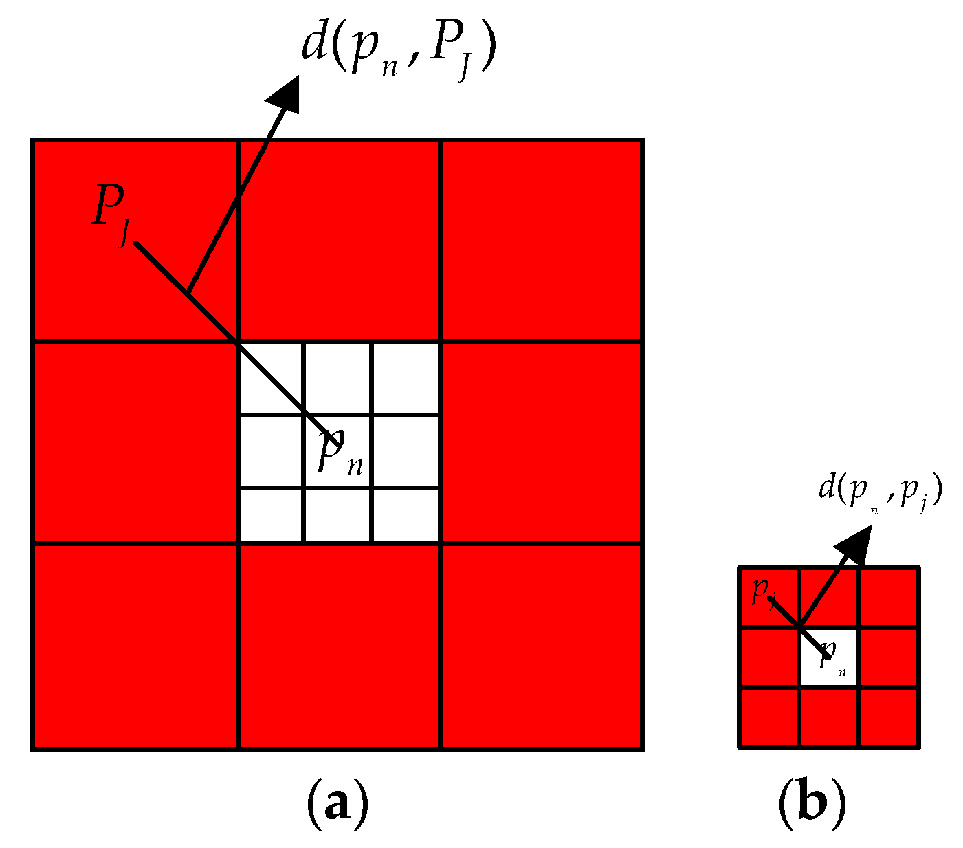
2. Theory of Spatial Correlation
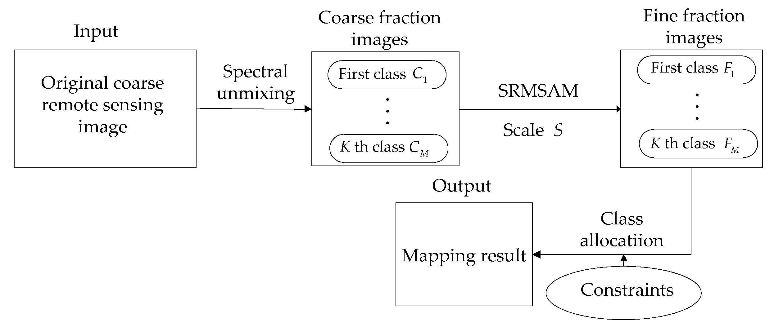
3. SRMSAM
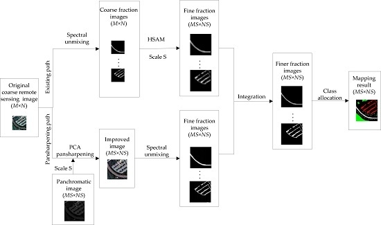
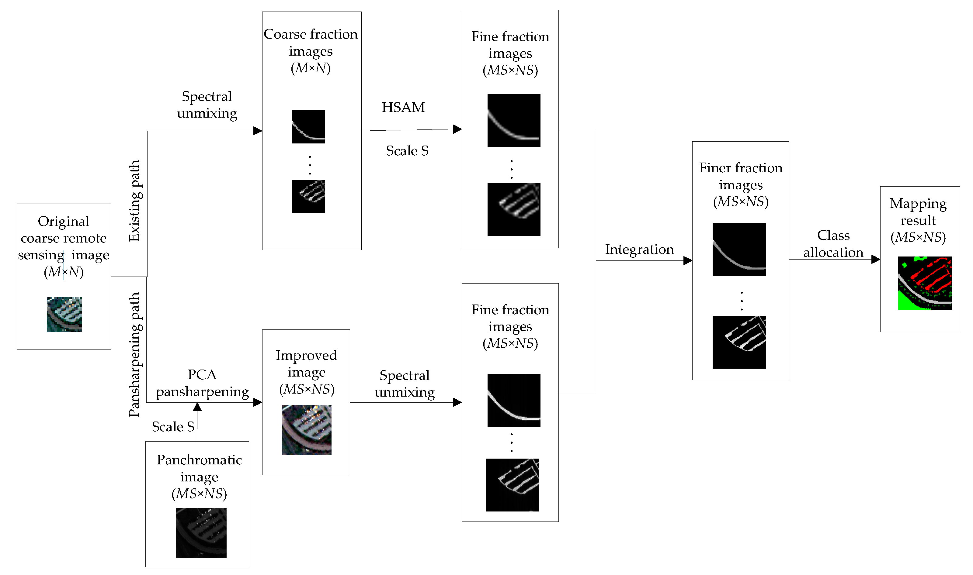
4. Proposed Method
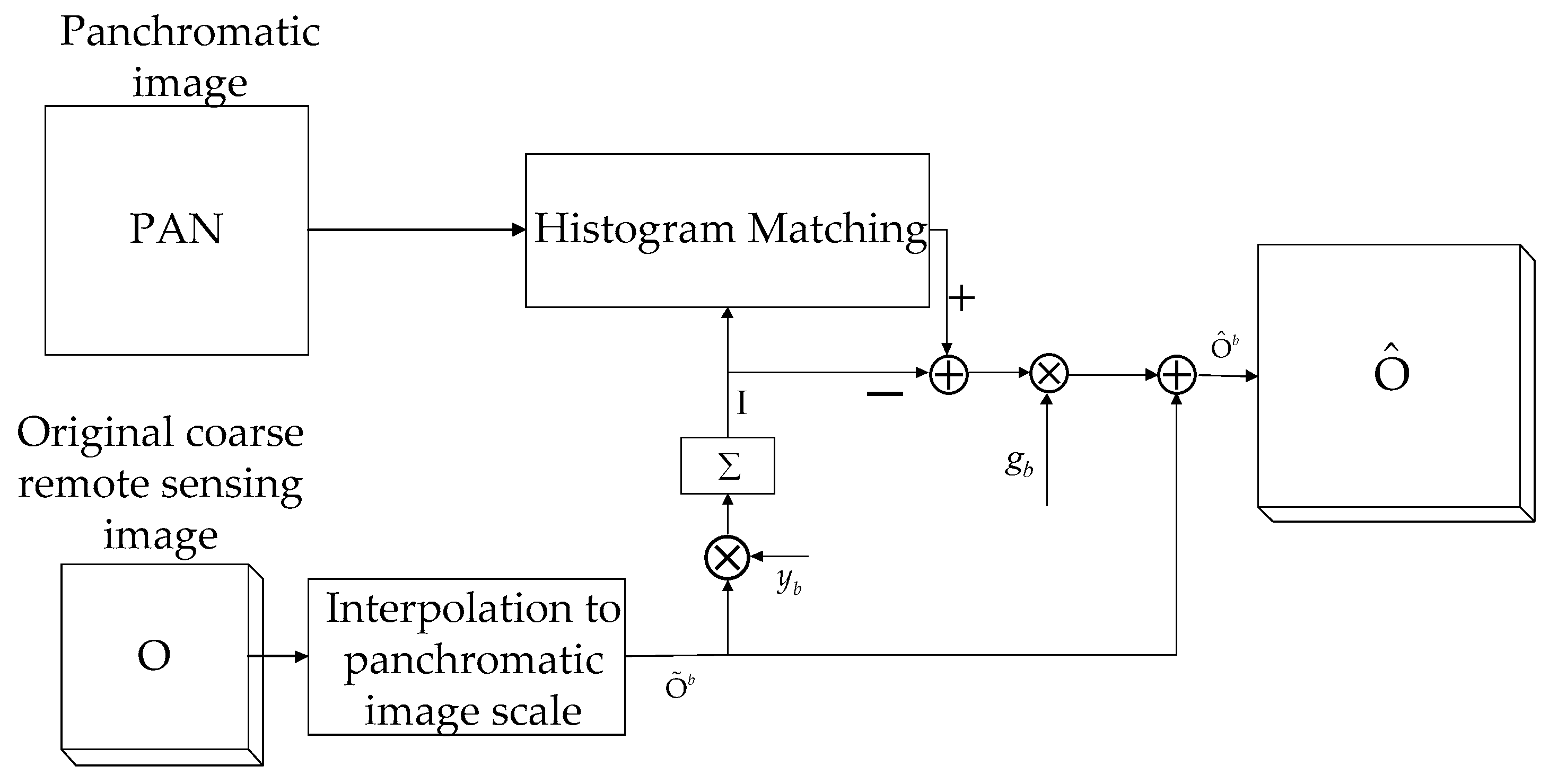
4.1. Pansharpening Path
4.2. Implementation of SRMSAM-PAN
5. Experiments and Analysis
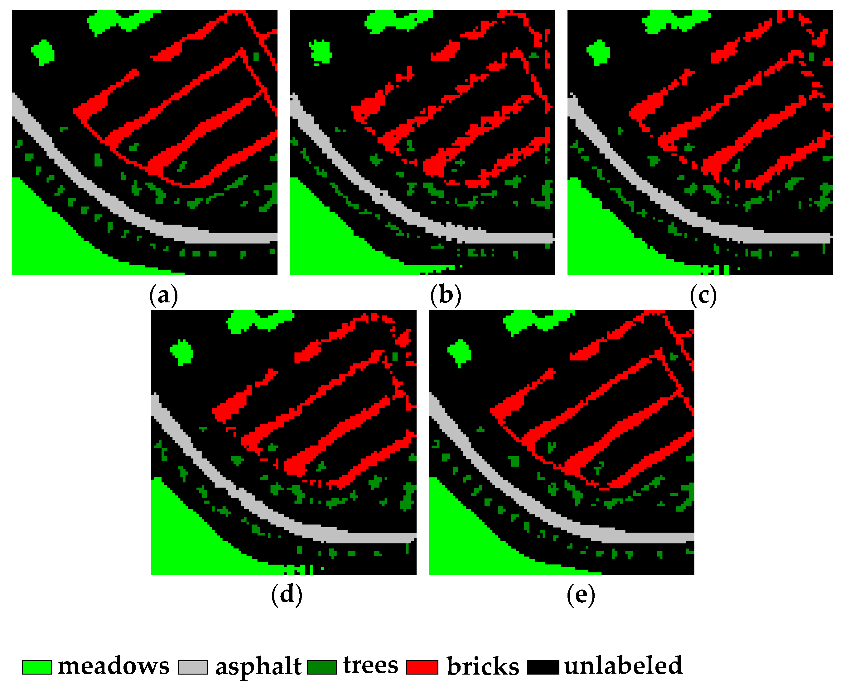
5.1. Experiment 1
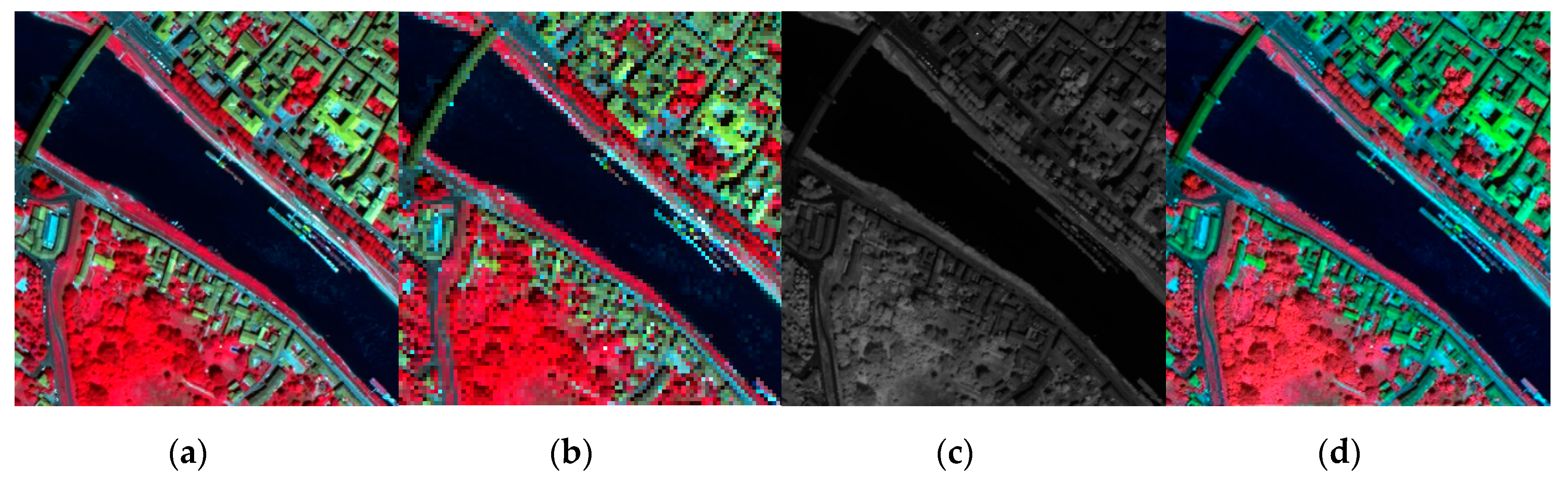
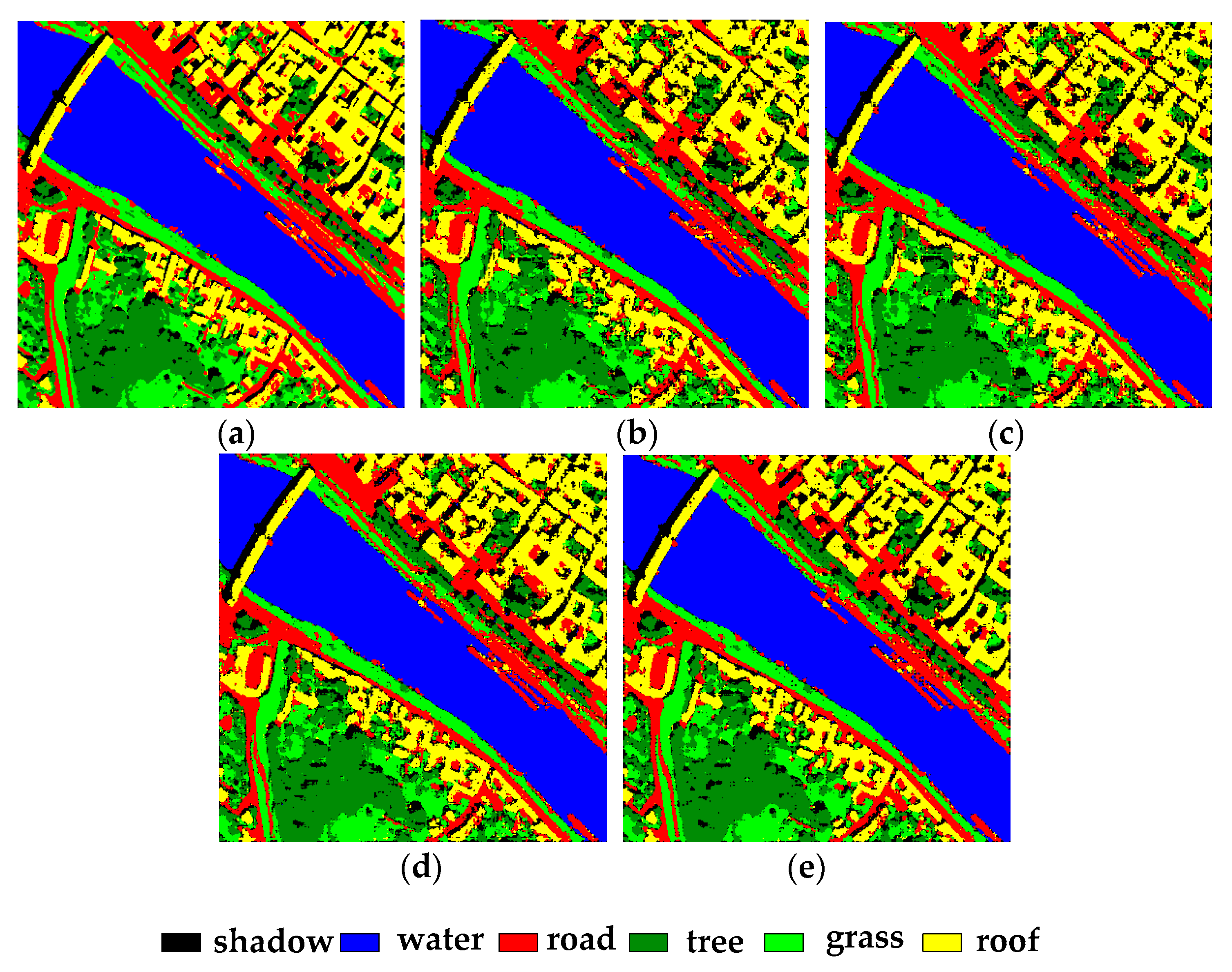
5.2. Experiment 2
5.3. Experiment 3
5.4. Discussion
6. Conclusions
Author Contributions
Funding
Acknowledgments
Conflicts of Interest
References
- Fisher, P. The pixel: A snare and a delusion. Int. J. Remote Sens. 1997, 18, 679–685. [Google Scholar] [CrossRef]
- Wang, L.; Liu, D.; Wang, Q. Geometric method of fully constrained least squares linear spectral mixture analysis. IEEE Trans. Geosci. Remote Sens. 2013, 51, 3558–3566. [Google Scholar] [CrossRef]
- Atkinson, P.M. Mapping sub-pixel boundaries from remotely sensed images. In Innovations in GIS; Taylor & Francis: New York, NY, USA, 1997; pp. 166–180. [Google Scholar]
- Ma, A.; Zhong, Y.; He, D.; Zhang, L. Multi-objective subpixel land-cover mapping. IEEE Trans. Geosci. Remote Sens. 2018, 56, 422–435. [Google Scholar] [CrossRef]
- Atkinson, P.M. Sub-pixel target mapping from soft-classified remotely sensed imagery. Photogramm. Eng. Remote Sens. 2005, 71, 839–846. [Google Scholar] [CrossRef]
- Tatem, A.J.; Lewis, H.G.; Atkinson, P.M.; Nixon, M.S. Super-resolution target identification form remotely sensed images using a Hopfield neural network. IEEE Trans. Geosci. Remote Sens. 2011, 39, 781–796. [Google Scholar] [CrossRef]
- Muad, A.M.; Foody, G.M. Impact of land cover patch size on the accuracy of patch area representation in HNN-based super resolution mapping. IEEE J. Sel. Top. Appl. Earth Observ. Remote Sens. 2012, 5, 1418–1427. [Google Scholar] [CrossRef]
- Shao, Y.; Lunetta, R.S. Sub-pixel mapping of tree canopy, impervious surfaces, and cropland in the Laurentian great lakes basin using MODIS time-series data. IEEE J. Sel. Top. Appl. Earth Observ. Remote Sens. 2011, 4, 336–347. [Google Scholar] [CrossRef]
- Nigussie, D.; Zurita-Milla, R.; Clevers, J.G.P.W. Possibilities and limitations of artificial neural networks for subpixel mapping of land cover. Int. J. Remote Sens. 2011, 32, 7203–7226. [Google Scholar] [CrossRef]
- Chen, Y.; Ge, Y.; Heuvelink, G.B.M.; An, R.; Chen, Y. Object-based superresolution land-cover mapping from remotely sensed imagery. IEEE Trans. Geosci. Remote Sens. 2018, 56, 328–340. [Google Scholar] [CrossRef]
- Chen, Y.; Zhou, Y.; Ge, Y.; An, R.; Chen, Y. Enhancing land cover mapping through integration of pixel-based and object-based classifications from remotely sensed imagery. Remote Sens. 2018, 10, 77. [Google Scholar] [CrossRef]
- Jin, H.; Mountrakis, G.; Li, P. A super-resolution mapping method using local indicator variograms. Int. J. Remote Sens. 2012, 33, 7747–7773. [Google Scholar] [CrossRef]
- Wang, Q.; Atkinson, P.M.; Shi, W. Indicator cokriging-based subpixel mapping without prior spatial structure information. IEEE Trans. Geosci. Remote Sens. 2015, 53, 309–323. [Google Scholar] [CrossRef]
- Wang, Q.; Atkinson, P.M. The effect of the point spread function on sub-pixel mapping. Remote Sens. Environ. 2017, 193, 127–137. [Google Scholar] [CrossRef]
- Chen, Y.; Ge, Y.; An, R.; Chen, Y. Super-resolution mapping of impervious surfaces from remotely sensed imagery with points-of-interest. Remote Sens. 2018, 10, 242. [Google Scholar] [CrossRef]
- Wang, P.; Zhang, G.; Kong, Y.; Leung, H. Superresolution mapping based on hybrid interpolation by parallel paths. Remote Sens. Lett. 2019, 10, 149–157. [Google Scholar] [CrossRef]
- Wang, Q.; Shi, W.; Atkinson, P.M. Spatiotemporal subpixel mapping of time-series images. IEEE Trans. Geosci. Remote Sens. 2016, 54, 5397–5411. [Google Scholar] [CrossRef]
- Wang, P.; Wang, L.; Chanussot, J. Soft-then-hard subpixel land cover mapping based on spatial-spectral interpolation. IEEE Geosci. Remote Sens. Lett. 2016, 13, 1851–1854. [Google Scholar] [CrossRef]
- Wang, Q.; Shi, W.; Wang, L. Allocating classes for soft-then-hard sub-pixel mapping algorithms in units of class. IEEE Trans. Geosci. Remote Sens. 2014, 5, 2940–2959. [Google Scholar] [CrossRef]
- Li, F.; Jia, X. Superresolution reconstruction of multispectral data for improved image classification. IEEE Geosci. Remote Sens. Lett. 2009, 5, 798–802. [Google Scholar]
- Wang, L.; Wang, P.; Zhao, C. Producing subpixel resolution thematic map from coarse imagery: MAP algorithm-based super-resolution recovery. IEEE J. Sel. Top. Appl. Earth Observ. Remote Sens. 2016, 9, 2290–2304. [Google Scholar] [CrossRef]
- Wang, P.; Wang, L.; Wu, Y.; Leung, H. Utilizing pansharpening technique to produce sub-pixel resolution thematic map from coarse remote sensing image. Remote Sens. 2018, 10, 884. [Google Scholar] [CrossRef]
- Wang, Q.; Wang, L.; Liu, D. Particle swarm optimization-based sub-pixel mapping for remote-sensing imagery. Int. J. Remote Sens. 2012, 33, 6480–6496. [Google Scholar] [CrossRef]
- Wang, P.; Zhang, G.; Leung, H. Improving super-resolution flood inundation mapping for multispectral remote sensing image by supplying more spectral information. IEEE Geosci. Remote Sens. Lett. 2018. [Google Scholar] [CrossRef]
- Zhang, Y.; Ling, F.; Li, X.; Du, Y. Super-resolution land cover mapping using multiscale self-similarity redundancy. IEEE J. Sel. Top. Appl. Earth Observ. Remote Sens. 2015, 8, 5130–5145. [Google Scholar] [CrossRef]
- Tong, X.; Xu, X.; Plaza, A.; Xie, H.; Pan, H.; Cao, W.; Lv, D. A new genetic method for subpixel mapping using hyperspectral images. IEEE J. Sel. Top. Appl. Earth Observ. Remote Sens. 2016, 9, 4480–4491. [Google Scholar] [CrossRef]
- Wang, Q.; Shi, W.; Atkinson, P.M. Sub-pixel mapping of remote sensing images based on radial basis function interpolation. ISPRS J. Photogramm. 2014, 92, 1–15. [Google Scholar] [CrossRef]
- Xu, X.; Zhong, Y.; Zhang, L.; Zhang, H. Sub-pixel mapping based on a MAP model with multiple shifted hyperspectral imagery. IEEE J. Sel. Top. Appl. Earth Observ. Remote Sens. 2013, 6, 580–593. [Google Scholar] [CrossRef]
- Wang, P.; Wang, L.; Mura, M.D.; Chanussot, J. Using multiple subpixel shifted images with spatial-spectral information in soft-then-hard subpixel mapping. IEEE J. Sel. Top. Appl. Earth Observ. Remote Sens. 2017, 13, 1851–1854. [Google Scholar] [CrossRef]
- Nguyen, M.Q.; Atkinson, P.M.; Lewis, H.G. Superresolution mapping using Hopfield neural network with LIDAR data. IEEE Geosci. Remote Sens. Lett. 2005, 2, 366–370. [Google Scholar] [CrossRef]
- Nguyen, M.Q.; Atkinson, P.M.; Lewis, H.G. Superresolution mapping using a Hopfield neural network with fused images. IEEE Trans. Geosci. Remote Sens. 2006, 44, 736–749. [Google Scholar] [CrossRef]
- Nguyen, M.Q.; Atkinson, P.M.; Lewis, H.G. Super-resolution mapping using Hopfield neural network with panchromatic imagery. Int. J. Remote Sens. 2011, 32, 6149–6176. [Google Scholar] [CrossRef]
- Thornton, M.W.; Atkinson, P.M.; Holland, D.A. A linearised pixel swapping method for mapping rural linear land cover features from fine spatial resolution remotely sensed imagery. Comput. Geosci. 2007, 33, 1261–1272. [Google Scholar] [CrossRef]
- Mertens, K.C.; Basets, B.D.; Verbeke, L.P.C.; De Wulf, R. A sub-pixel mapping algorithm based on sub-pixel/pixel spatial attraction models. Int. J. Remote Sens. 2006, 27, 3293–3310. [Google Scholar] [CrossRef]
- Ling, F.; Li, X.; Du, Y.; Xiao, F. Sub-pixel mapping of remotely sensed imagery with hybrid intra- and inter-pixel dependence. Int. J. Remote Sens. 2013, 34, 341–357. [Google Scholar] [CrossRef]
- Wang, P.; Wang, L. Soft-then-hard super-resolution mapping based on a spatial attraction model with multiscale sub-pixel shifted images. Int. J. Remote Sens. 2017, 38, 4303–4326. [Google Scholar] [CrossRef]
- Vivone, G.; Alparone, L.; Chanussot, J.; Mura, M.D.; Garzelli, A.; Licciardi, G.; Restaino, R.; Wald, L. A critical comparison among pansharpening algorithms. IEEE Trans. Geosci. Remote Sens. 2015, 53, 2565–2585. [Google Scholar] [CrossRef]
- Wang, L.; Liu, D.; Wang, Q. Spectral unmixing model based on least squares support vector machine with unmixing residue constraints. IEEE Geosci. Remote Sens. Lett. 2013, 10, 1592–1596. [Google Scholar] [CrossRef]
- Wang, P.; Zhang, G.; Leung, H. Utilizing parallel networks to produce sub-pixel shifted images with multiscale spatio-spectral information for soft-then-hard sub-pixel mapping. IEEE Access. 2018, 6, 57485–57496. [Google Scholar] [CrossRef]
- Thomas, C.; Ranchin, T.; Wald, L.; Chanussot, J. Synthesis of multispectral images to high spatial resolution: A critical review of fusion methods based on remote sensing physics. IEEE Trans. Geosci. Remote Sens. 2008, 46, 1301–1312. [Google Scholar] [CrossRef]
- Ge, Y.; Chen, Y.; Stein, A.; Li, S.; Hu, J. Enhanced sub-pixel mapping with spatial distribution patterns of geographical objects. IEEE Trans. Geosci. Remote Sens. 2016, 54, 2356–2370. [Google Scholar] [CrossRef]
- Zhang, L.; Zhang, L.; Tao, D.; Huang, X. Tensor discriminative locality alignment for hyperspectral image spectral-spatial feature extraction. IEEE Trans. Geosci. Remote Sens. 2013, 51, 242–256. [Google Scholar] [CrossRef]
- Garzelli, A.; Nencini, F.; Capobianco, L. Optimal MMSE pan sharpening of very high resolution multispectral images. IEEE Trans. Geosci. Remote Sens. 2008, 46, 228–236. [Google Scholar] [CrossRef]


| SPSAM | MSPSAM | HSAM | SRMSAM-PAN | |
|---|---|---|---|---|
| Meadows | 96.37 | 97.10 | 97.73 | 99.13 |
| Asphalt | 95.48 | 97.29 | 97.47 | 99.82 |
| Tress | 45.13 | 55.23 | 56.32 | 72.31 |
| Bricks | 77.18 | 83.37 | 83.60 | 90.30 |
| OA | 85.17 | 88.73 | 89.20 | 93.87 |
| SPSAM | MSPSAM | HSAM | SRMSAM-PAN | |
|---|---|---|---|---|
| Shadow | 52.46 | 62.80 | 65.98 | 74.57 |
| Water | 98.04 | 98.33 | 98.35 | 98.76 |
| Road | 79.38 | 82.97 | 84.03 | 89.74 |
| Tree | 80.95 | 83.47 | 84.52 | 89.00 |
| Grass | 80.51 | 83.94 | 85.66 | 89.41 |
| Roof | 85.89 | 88.63 | 89.87 | 92.49 |
| OA | 88.52 | 90.86 | 92.20 | 95.11 |
© 2019 by the authors. Licensee MDPI, Basel, Switzerland. This article is an open access article distributed under the terms and conditions of the Creative Commons Attribution (CC BY) license (http://creativecommons.org/licenses/by/4.0/).
Share and Cite
Wang, P.; Zhang, G.; Hao, S.; Wang, L. Improving Remote Sensing Image Super-Resolution Mapping Based on the Spatial Attraction Model by Utilizing the Pansharpening Technique. Remote Sens. 2019, 11, 247. https://doi.org/10.3390/rs11030247
Wang P, Zhang G, Hao S, Wang L. Improving Remote Sensing Image Super-Resolution Mapping Based on the Spatial Attraction Model by Utilizing the Pansharpening Technique. Remote Sensing. 2019; 11(3):247. https://doi.org/10.3390/rs11030247
Chicago/Turabian StyleWang, Peng, Gong Zhang, Siyuan Hao, and Liguo Wang. 2019. "Improving Remote Sensing Image Super-Resolution Mapping Based on the Spatial Attraction Model by Utilizing the Pansharpening Technique" Remote Sensing 11, no. 3: 247. https://doi.org/10.3390/rs11030247
APA StyleWang, P., Zhang, G., Hao, S., & Wang, L. (2019). Improving Remote Sensing Image Super-Resolution Mapping Based on the Spatial Attraction Model by Utilizing the Pansharpening Technique. Remote Sensing, 11(3), 247. https://doi.org/10.3390/rs11030247