Analysis of Physical and Biogeochemical Control Mechanisms on Summertime Surface Carbonate System Variability in the Western Ross Sea (Antarctica) Using In Situ and Satellite Data

 , , and
Abstract
1. Introduction
2. Materials and Methods
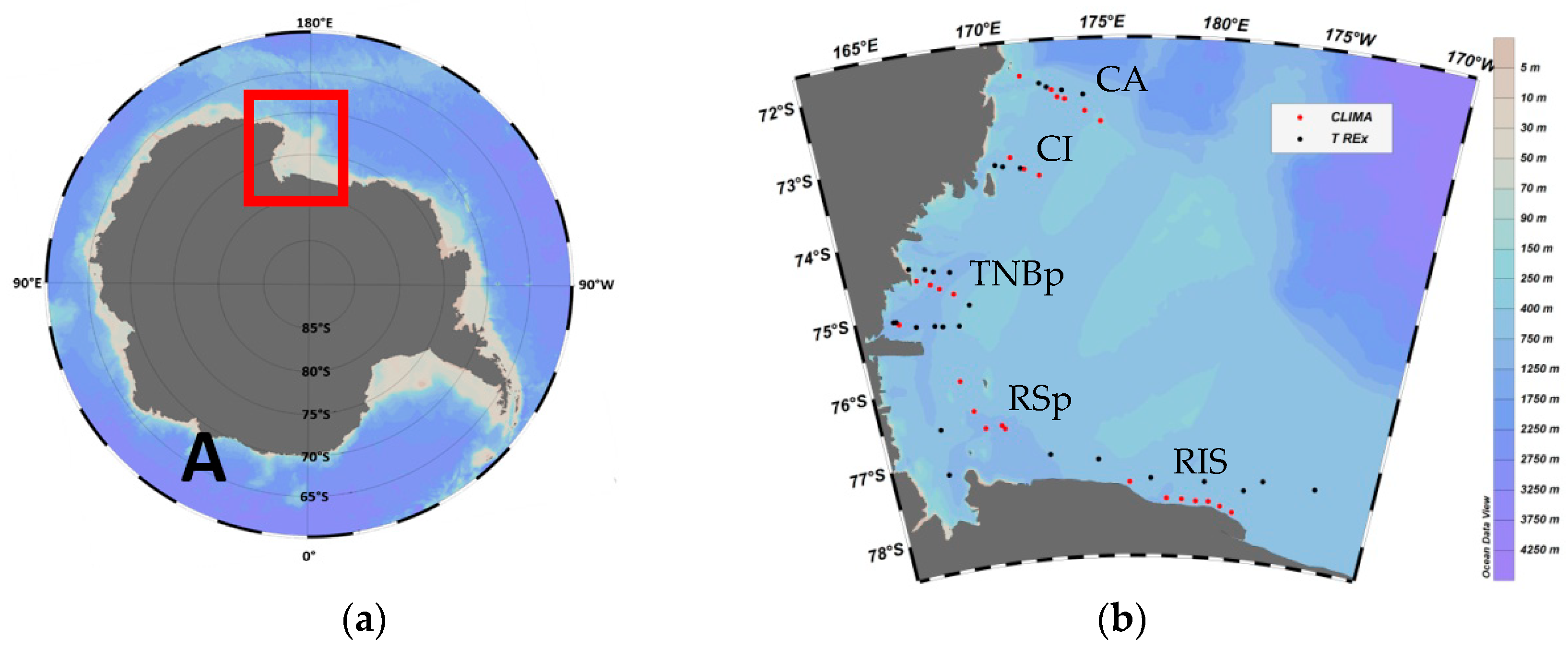
2.1. Sampling
2.2. AT, CT, and pH Measurements
2.3. CO2 -Carbonate System
2.4. Hydrographic and Ancillary Data
2.5. Statistical Analysis
2.6. Satellite Data
3. Results
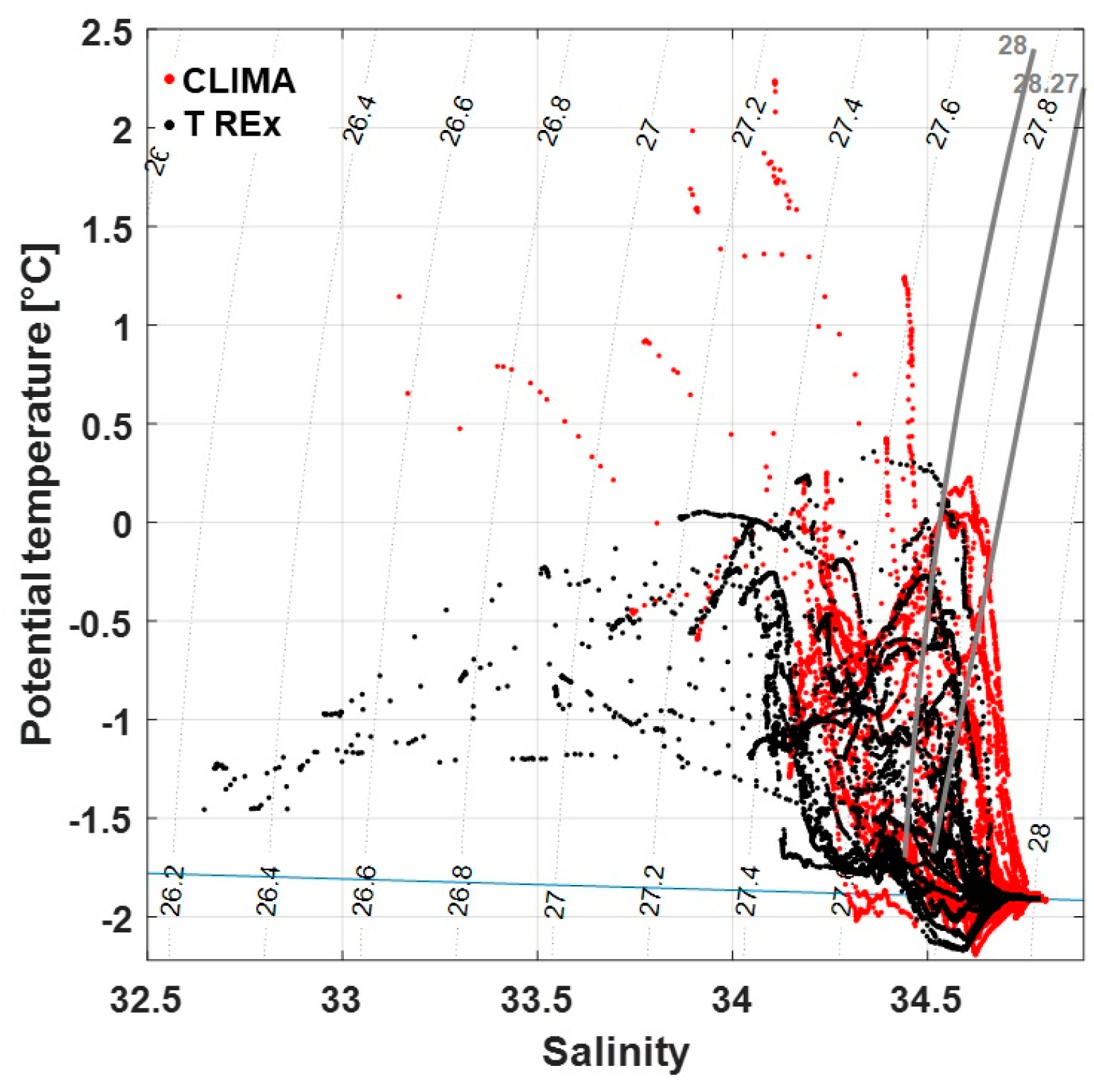
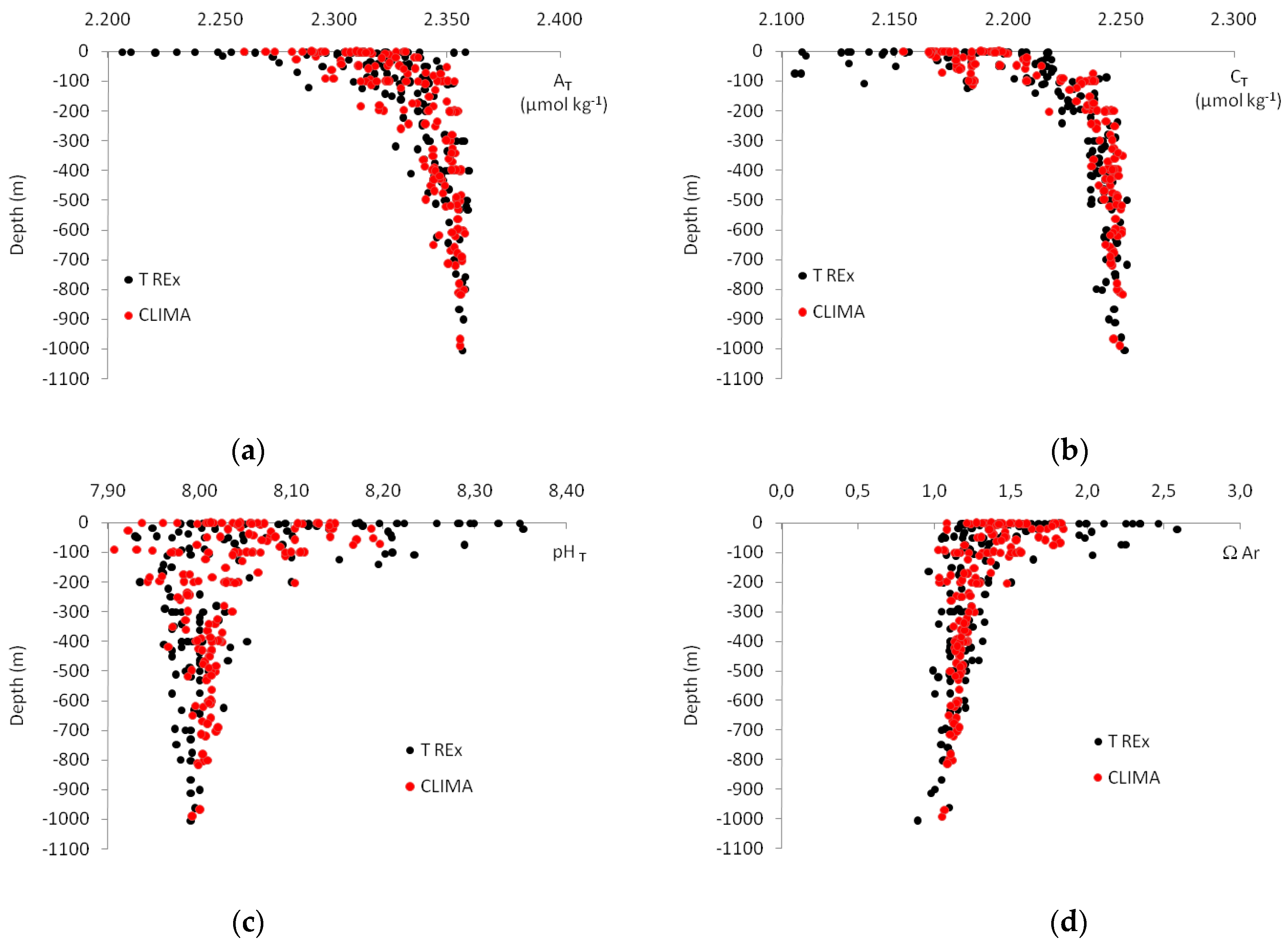
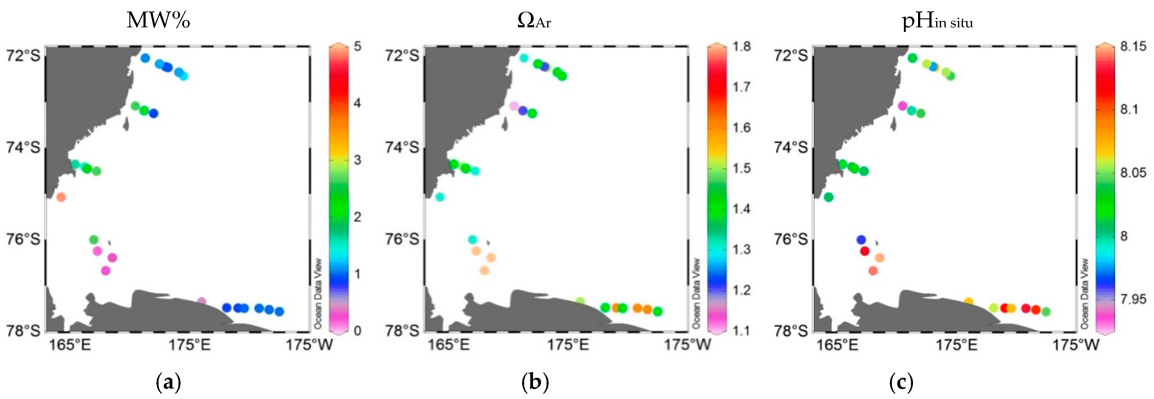
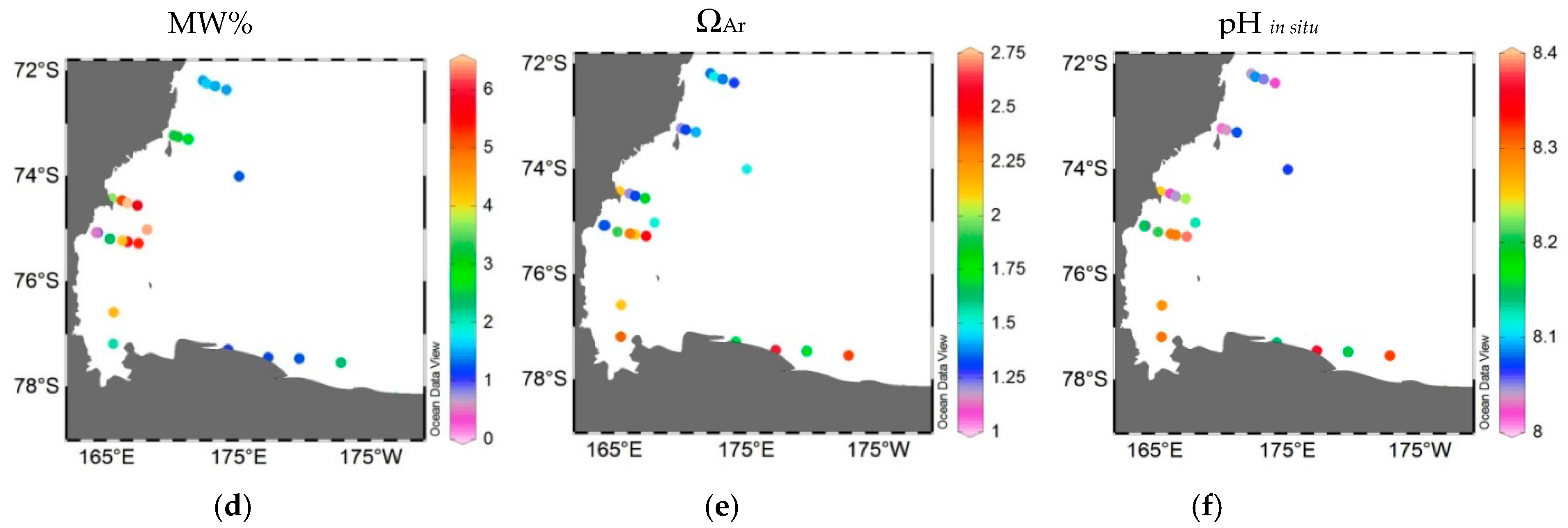
3.1. Hydrographic and Carbonate Chemistry Variability
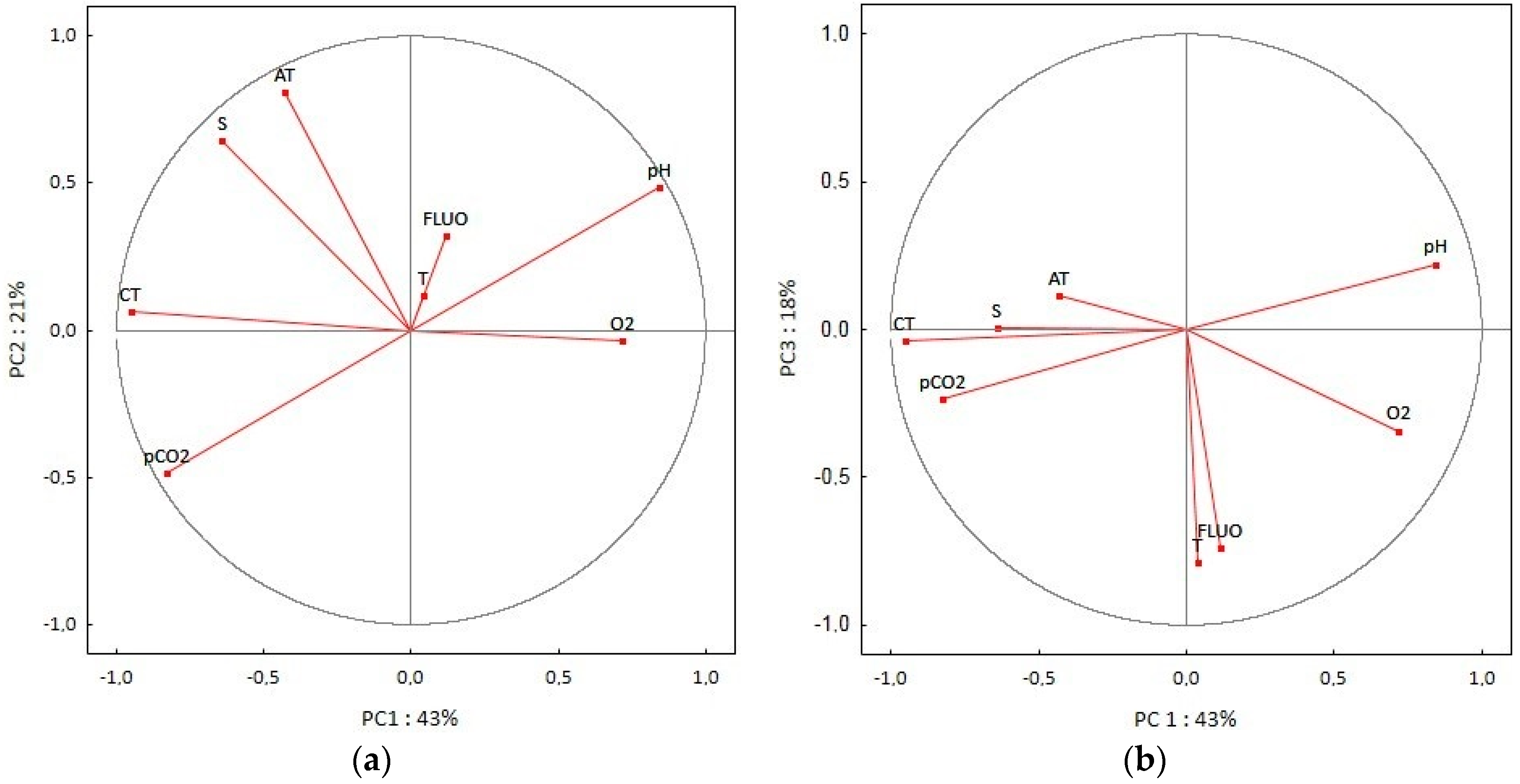
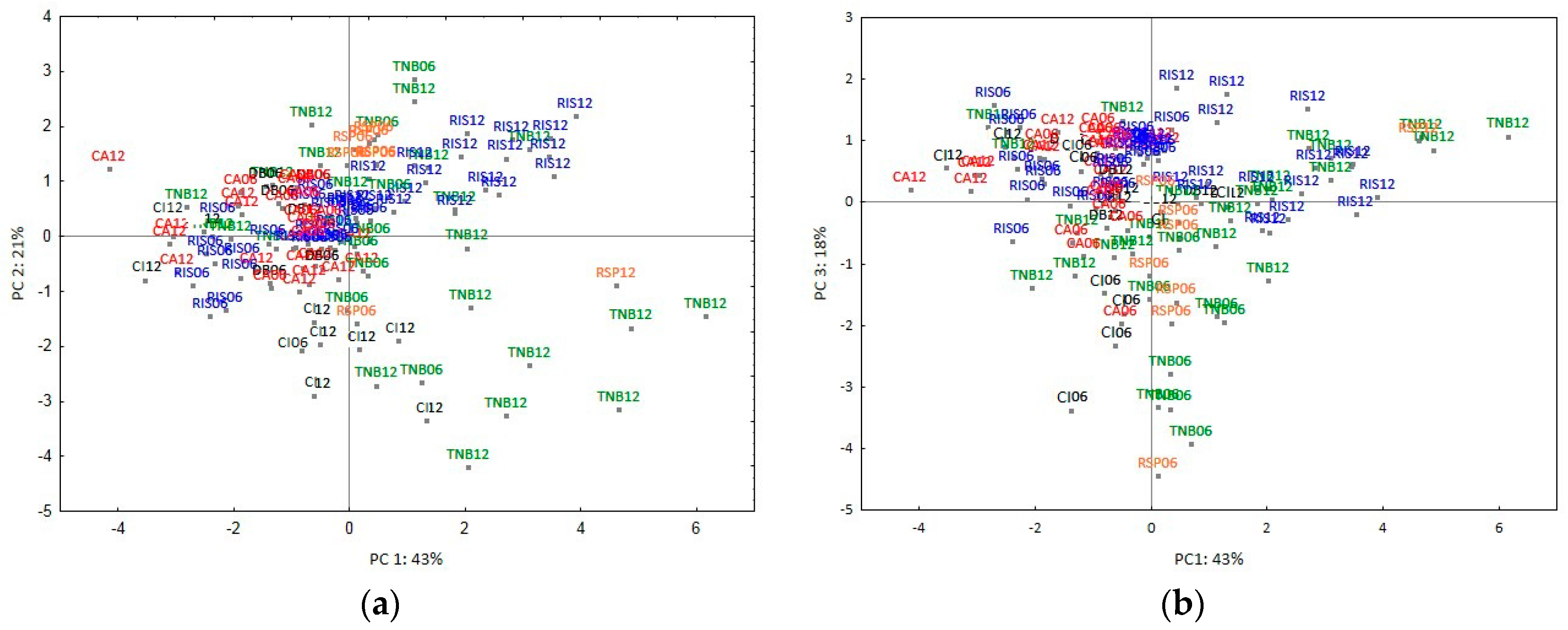
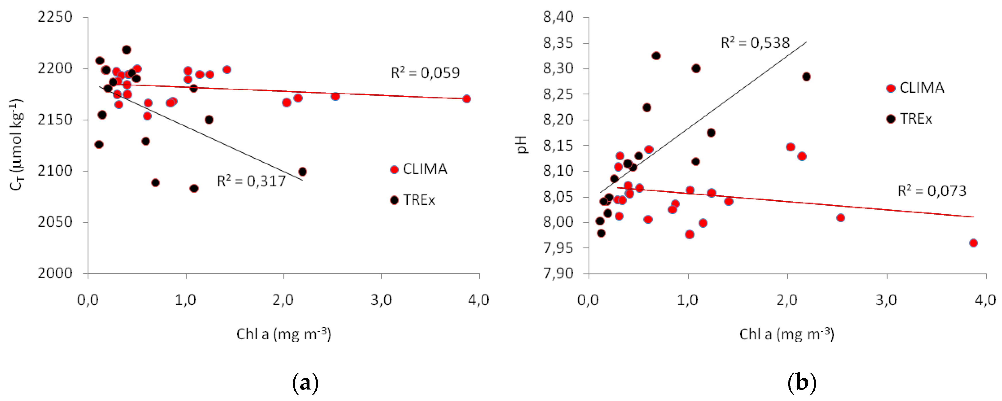
3.2. Data Analysis
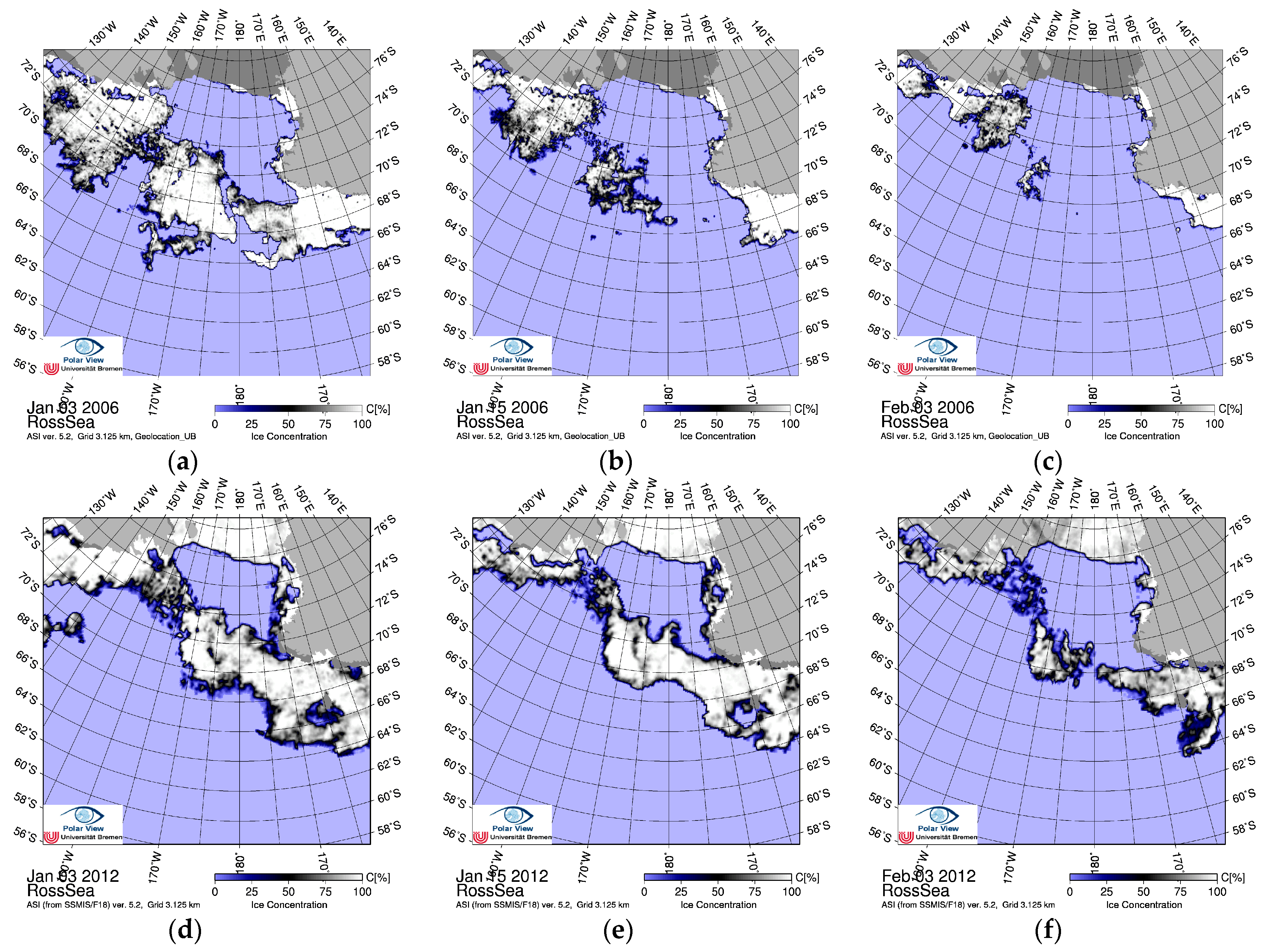
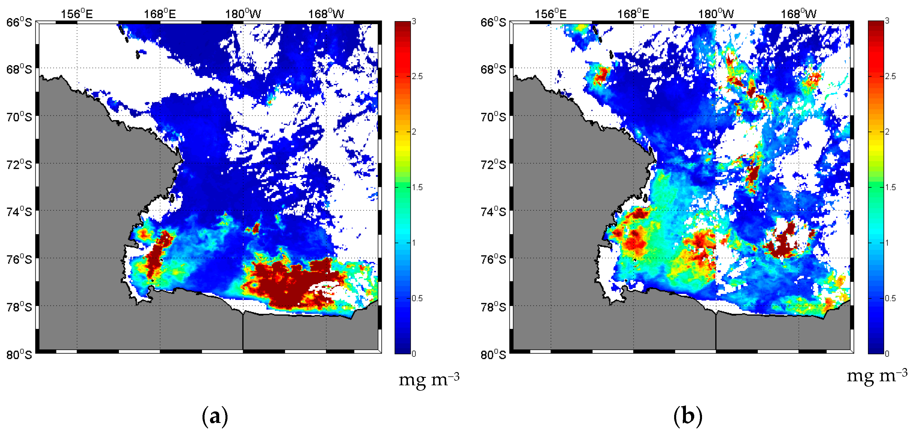
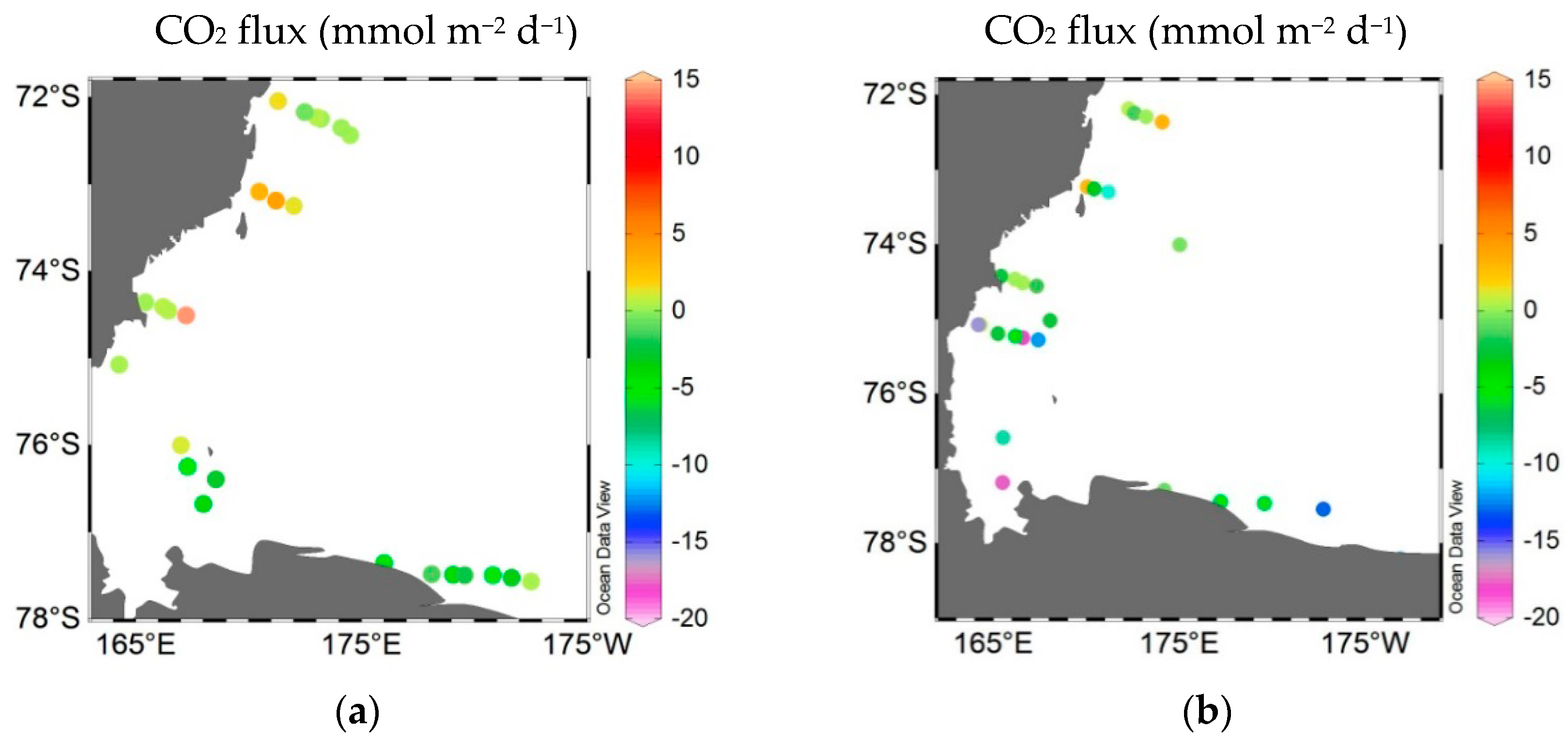
3.3. Satellite Data
4. Discussion
4.1. Physically-Induced Variability of the Carbonate System in the AASW
4.2. Biologically-Induced Variability of the Carbonate System in the AASW
5. Conclusions
Author Contributions
Funding
Acknowledgments
Conflicts of Interest
References
- Sabine, C.L.; Feely, R.A.; Gruber, N.; Key, R.M.; Lee, K.; Bullister, J.L.; Wanninkhof, R.; Wong, C.S.; Wallace, D.W.R.; Tilbrook, B.; et al. The oceanic sink for anthropogenic CO2. Science 2004, 305, 367–371. [Google Scholar] [CrossRef] [PubMed]
- Jones, E.M.; Fenton, M.; Meredith, M.P.; Clargo, N.M.; Ossebaar, S.; Ducklow, H.W.; Venables, H.J.; de Baar, H.J.W. Ocean acidification and calcium carbonate saturation states in the coastal zone of the West Antarctic Peninsula. Deep-Sea Res. Part II 2017, 139, 181–194. [Google Scholar] [CrossRef]
- Feely, R.A.; Sabine, C.L.; Lee, K.; Berelson, W.; Kleypas, J.; Fabry, V.J.; Millero, F.J. Impact of anthropogenic CO2 on the CaCO3 system in the oceans. Science 2004, 305, 362–366. [Google Scholar] [CrossRef] [PubMed]
- Cao, L.; Caldeira, K.; Jain, A.K. Effects of carbon dioxide and climate change on ocean acidification and carbonate mineral saturation. Geophys. Res. Lett. 2007, 34, L05607. [Google Scholar] [CrossRef]
- Orr, J.C.; Fabry, V.J.; Aumont, O.; Bopp, L.; Doney, S.C.; Feely, R.A.; Gnanadesikan, A.; Gruber, N.; Ishida, A.; Joos, F.; et al. Anthropogenic ocean acidification over the twenty-first century and its impact on calcifying organisms. Nature 2005, 437, 681–686. [Google Scholar] [CrossRef] [PubMed]
- Feely, R.; Doney, S.; Cooley, S. Ocean Acidification: Present conditions and future changesin a high-CO2 world. Oceanography 2009, 22, 36–47. [Google Scholar] [CrossRef]
- Manno, C.; Sandrini, S.; Tositti, L.; Accornero, A. First stages of degradation of Limacina helicina shells observed above the aragonite chemical lysocline in Terra Nova Bay (Antarctica). J. Mar. Syst. 2007, 68, 91–102. [Google Scholar] [CrossRef]
- Bednaršek, N.; Tarling, G.A.; Bakker, D.C.E.; Fielding, S.; Jones, E.M.; Venables, H.J.; Ward, P.; Kuzirian, A.; Lézé, B.; Feely, R.A.; et al. Extensive dissolution of live pteropods in the Southern Ocean. Nat. Geosci. 2012, 5, 881–885. [Google Scholar] [CrossRef]
- Schine, C.M.S.; van Dijken, G.L.; Arrigo, K.R. Spatial analysis of trends in primary production and relationship with large-scale climate variability in the Ross Sea, Antarctica (1997±2013). J. Geophys. Res. Oceans 2016, 121, 368–386. [Google Scholar] [CrossRef]
- Smith, W.O., Jr.; Ainley, D.G.; Arrigo, K.R.; Dinniman, M.S. The Oceanography and Ecology of the Ross Sea. Annu. Rev. Mar. Sci. 2014, 6, 469–487. [Google Scholar] [CrossRef]
- Budillon, G.; Pacciaroni, M.; Cozzi, S.; Rivaro, P.; Catalano, G.; Ianni, C.; Cantoni, C. An optimum multiparameter mixing analysis of the shelf waters in the Ross Sea. Antarct. Sci. 2003, 15, 105–118. [Google Scholar] [CrossRef]
- Orsi, A.H.; Wiederwohl, C.L. A recount of Ross Sea waters. Deep-Sea Res. Part II 2009, 56, 778–795. [Google Scholar] [CrossRef]
- Arrigo, K.R.; van Dijken, G.; Long, M. Coastal Southern Ocean: A strong anthropogenic CO2 sink. Geophys. Res. Lett. 2008, 35, L21602. [Google Scholar] [CrossRef]
- Caldeira, K.; Duffy, P.B. The role of the Southern Ocean in uptake and storage of anthropogenic carbon dioxide. Science 2000, 287, 620–622. [Google Scholar] [CrossRef]
- Tortell, P.D.; Guéguen, C.; Long, M.C.; Payne, C.D.; Leeand, P.; Di Tullio, G.R. Spatial variability and temporal dynamics of surface water pCO2, ∆O2/Ar and dimethylsulfide inthe Ross Sea, Antarctica. Deep-Sea Res. Part II 2011, 58, 241–259. [Google Scholar] [CrossRef]
- Bates, N.R.; Hansell, D.A.; Carlson, C.A.; Gordon, L.I. Distribution of CO2 species, estimates of net community production, and air-sea CO2 exchange in the Ross Sea polynya. J. Geophys. Res. 1998, 103, 2883–2896. [Google Scholar] [CrossRef]
- Sweeney, C.; Hansell, D.A.; Carlson, C.A.; Codispoti, L.A.; Gordon, L.I.; Marra, J.; Millero, F.J.; Smith, W.O., Jr.; Takahashi, T. Biogeochemical regimes, net community production and carbon export in the Ross Sea, Antarctica. Deep-Sea Res. Part II 2000, 47, 3369–3394. [Google Scholar] [CrossRef]
- Sandrini, S.; Aït-Ameur, N.; Rivaro, P.; Massolo, S.; Touratier, F.; Tositti, L.; Goyet, C. Anthropogenic carbon distribution in the Ross Sea (Antarctica). Antarct. Sci. 2007, 19, 395–407. [Google Scholar] [CrossRef]
- Kapsenberg, L.; Kelley, A.L.; Shaw, E.C.; Martz, T.R.; Hofmann, G.E. Near-shore Antarctic pH variability has implications for the design of ocean acidification experiments. Sci. Rep. 2015, 5, 9638–9647. [Google Scholar] [CrossRef]
- Rivaro, P.; Ianni, C.; Langone, L.; Ori, C.; Aulicino, G.; Cotroneo, Y.; Saggiomo, M.; Mangoni, O. Physical and biological forcing of mesoscale variability in the carbonate system of the Ross Sea (Antarctica) during summer 2014. J. Mar. Syst. 2017, 166, 144–168. [Google Scholar] [CrossRef]
- Mattsdotter Björk, M.; Fransson, A.; Torstensson, A.; Chierici, M. Ocean acidification state in western Antarctic surface waters: Controls and interannual variability. Biogeosciences 2014, 11, 57–73. [Google Scholar] [CrossRef]
- Conrad, C.J.; Lowenduski, N. Climate-driven variability in the Southern Ocean carbonate system. J. Clim. 2015, 28, 5335–5350. [Google Scholar] [CrossRef]
- Buongiorno Nardelli, B.; Guinehut, S.; Verbrugge, N.; Cotroneo, Y.; Zambianchi, E.; Iudicone, D. Southern Ocean mixed layer seasonal and interannual variations from combined satellite and in situ data. J. Geophys. Res. Oceans 2017, 122, 10042–10060. [Google Scholar] [CrossRef]
- Cerrone, D.; Fusco, G.; Cotroneo, Y.; Simmonds, I.; Budillon, G. The Antarctic Circumpolar Wave: Its presence and interdecadal changes during the last 142 Years. J. Clim. 2017, 30, 6371–6389. [Google Scholar] [CrossRef]
- Cerrone, D.; Fusco, G.; Simmonds, I.; Aulicino, G.; Budillon, G. Dominant covarying climate signals in the Southern Ocean and Antarctic sea ice influence during the last three decades. J. Clim. 2017, 30, 3055–3072. [Google Scholar] [CrossRef]
- Fusco, G.; Cotroneo, Y.; Aulicino, G. Different behaviors of the Ross and Weddell Seas surface heat fluxes in the period 1972–2015. Climate 2018, 6, 17. [Google Scholar] [CrossRef]
- Aulicino, G.; Cotroneo, Y.; Ruiz, S.; Román, A.S.; Pascual, A.; Fusco, G.; Tintoré, J. Monitoring the Algerian Basin through glider observations, satellite altimetry and numerical simulations along a SARAL/AltiKa track. J. Mar. Syst. 2018, 179, 55–71. [Google Scholar] [CrossRef]
- Cotroneo, Y.; Budillon, G.; Fusco, G.; Spezie, G. Cold core eddies and fronts of the Antarctic Circumpolar Current south of New Zealand from in situ and satellite data. J. Geophys. Res. 2013, 118, 2653–2666. [Google Scholar] [CrossRef]
- Cotroneo, Y.; Aulicino, G.; Ruiz, S.; Pascual, A.; Budillon, G.; Fusco, G.; Tintoré, J. Glider and satellite high resolution monitoring of a mesoscale eddy in the Algerian basin: Effects on the mixed layer depth and biochemistry. J. Mar. Syst. 2015, 162, 73–88. [Google Scholar] [CrossRef]
- Dickson, A.G.; Sabine, C.L.; Christian, J.R. (Eds.) Guide to Best Practices for Ocean CO2 Measurements. PICES Spec. Publ. 2007, 3, 191. [Google Scholar] [CrossRef]
- Edmond, J.M. High precision determination of titration alkalinity and total carbon dioxide content of seawater by potentiometric titration. Deep-Sea Res. 1970, 17, 737–750. [Google Scholar]
- Rivaro, P.; Messa, R.; Massolo, S.; Frache, R. Distributions of carbonate properties along the water column in the Mediterranean Sea: Spatial and temporal variations. Mar. Chem. 2010, 121, 236–245. [Google Scholar] [CrossRef]
- Rivaro, P.; Messa, R.; Ianni, C.; Magi, E.; Budillon, G. Distribution of total alkalinity and pH in the Ross Sea (Antarctica) waters during austral summer 2008. Polar Res. 2014, 33, 20403. [Google Scholar] [CrossRef]
- Pierrot, D.; Lewis, E.; Wallace, D.W.R. MS Excel Program developed for CO2 system calculations, ORNL/CDIAC-105; Carbon Dioxide Information Analysis Center, Oak Ridge National Laboratory, US Department of Energy: Oak Ridge, TN, USA, 2006. [CrossRef]
- Millero, F.J.; Pierrot, D.; Lee, K.; Wanninkhof, R.; Feely, R.A.; Sabine, C.L.; Key, R.M.; Takahashi, T. Dissociation constants for carbonic acid determined from field measurements. Deep Sea Res. I 2002, 49, 1705–1723. [Google Scholar] [CrossRef]
- Wanninkhof, R. Relationship between wind speed and gas exchange over the ocean. J. Geophys. Res. Oceans 1992, 97, 7373–7382. [Google Scholar] [CrossRef]
- SCOR Working Group 51. The acquisition, calibration, and analysis of CTD data. UNESCO Tech. Pap. Mar. Sci. 1988, 54, 102. [Google Scholar]
- Fofonoff, N.P.; Millard, R.C., Jr. Algorithms for the computation of fundamental properties of seawater. UNESCO Tech. Pap. Mar. Sci. 1983, 44, 53. [Google Scholar]
- Rivaro, P.; Ianni, C.; Magi, E.; Massolo, S.; Budillon, G.; Smethie, W.M., Jr. Distribution and ventilation of water masses in the western Ross Sea inferred from CFC measurements. Deep-Sea Res. I 2015, 97, 19–28. [Google Scholar] [CrossRef]
- Mitchell, B.G.; Holm-Hansen, O. Observation and modelling of the Antarctic phytoplankton crop in relation to mixing depth. Deep Sea Res. I 1991, 38, 981–1007. [Google Scholar] [CrossRef]
- Mangoni, O.; Saggiomo, V.; Bolinesi, F.; Margiotta, F.; Budillon, G.; Cotroneo, Y.; Misic, C.; Rivaro, P.; Saggiomo, M. Phytoplankton blooms during austral summer in the Ross Sea, Antarctica: Driving factors and trophic implications. PLoS ONE 2017, 12, e0176033. [Google Scholar] [CrossRef]
- Farnham, I.M.; Johannesson, K.H.; Singh, A.K.; Hodge, V.F.; Stetzenbach, K.J. Factor analytical approaches for evaluating groundwater trace element chemistry data. Anal. Chim. Acta 2003, 490, 123–138. [Google Scholar] [CrossRef]
- Schlitzer, R. Ocean Data View 2015. Available online: http://odv.awi.de/ (accessed on 16 April 2016).
- Spreen, G.; Kaleschke, L.; Heygster, G. Sea ice remote sensing using AMSR-E 89 GHz channels. J. Geophys. Res. 2008, 113, C02S03. [Google Scholar] [CrossRef]
- Jackett, R.; McDougall, T.J. A neutral density variable for the world’s oceans. J. Phys. Oceanogr. 1997, 27, 237–263. [Google Scholar] [CrossRef]
- Castagno, P.; Falco, P.; Dinniman, M.S.; Spezie, G.; Budillon, G. Temporal variability of the Circumpolar Deep Water inflow onto the Ross Sea continental shelf. J. Mar. Syst. 2017, 166, 37–49. [Google Scholar] [CrossRef]
- Fusco, G.; Budillon, G.; Spezie, G. Surface heat fluxes and thermohaline variability in the Ross Sea and in Terra Nova Bay polynya. Cont. Shelf Res. 2009, 29, 1887–1895. [Google Scholar] [CrossRef]
- Rusciano, E.; Budillon, G.; Fusco, G.; Spezie, G. Evidence of atmosphere-sea ice- ocean coupling in the Terra Nova Bay polynya Ross Sea—Antarctica. Cont. Shelf Res. 2013, 61–62, 112–124. [Google Scholar] [CrossRef]
- DeJong, H.B.; Dunbar, R.B.; Mucciarone, D.A.; Koweek, D.A. Carbonate saturation state of surface waters in the Ross Sea and Southern Ocean: Controls and implications for the onset of aragonite undersaturation. Biogeosciences 2015, 12, 8429–8465. [Google Scholar] [CrossRef]
- Massolo, S.; Messa, R.; Rivaro, P.; Leardi, R. Annual and spatial variations of chemical and physical properties in the Ross Sea surface waters (Antarctica). Cont. Shelf Res. 2009, 29, 2333–2344. [Google Scholar] [CrossRef]
- Mo, K.C.; Ghil, M. Statistics and dynamics of persistent anomalies. J. Atmos. Sci. 1987, 44, 877–901. [Google Scholar] [CrossRef]
- Fogt, R.L.; Bromwich, D.H.; Hines, K.M. Understanding the SAM influence on the South Pacific ENSO teleconnection. Clim. Dyn. 2011, 36, 1555–1576. [Google Scholar] [CrossRef]
- Stammerjohn, S.E.; Martinson, D.G.; Smith, R.C.; Yuan, X.; Rind, D. Trends in Antarctic annual sea ice retreat and advance and their relation to El Niño–Southern Oscillation and Southern Annular Mode variability. J. Geophys. Res. 2008, 113, C03S90. [Google Scholar] [CrossRef]
- Parkinson, C.L. Southern Ocean sea ice and its wider linkages: Insights revealed from models and observations. Antarct. Sci. 2004, 16, 387–400. [Google Scholar] [CrossRef]
- Cerrone, D.; Fusco, G. Low-Frequency Climate Modes and Antarctic Sea Ice Variations, 1982-2013. J. Clim. 2018, 31, 147–175. [Google Scholar] [CrossRef]
- Raphael, M.N.; Marshall, G.J.; Turner, R.L.; Fogt, D.; Schneider, D.A.; Dixon, J.S.; Hosking, J.; Jones, M.; Hobbs, W.R. The Amundsen Sea low variability, change, and impact on Antarctic Climate. BAMS 2016, 97, 111–121. [Google Scholar] [CrossRef]
- Soppa, M.; Völker, C.; Bracher, A. Diatom phenology in the Southern Ocean: Mean patterns, trends and the role of climate oscillations. Remote Sens. 2016, 8, 420. [Google Scholar] [CrossRef]
- Chierici, M.; Fransson, A. CaCO3 saturation in the surface water of the Arctic Ocean: Undersaturation in freshwater influenced shelves. Biogeosciences 2009, 6, 2421–2432. [Google Scholar] [CrossRef]
- Gerringa, L.J.A.; Laan, P.; van Dijken, G.L.; van Haren, H.; De Baar, H.J.W.; Arrigo, K.R.; Alderkamp, A.C. Sources of iron in the Ross Sea Polynya in early summer. Mar. Chem. 2015, 177, 447–459. [Google Scholar] [CrossRef]
- Lannuzel, D.; Grotti, M.; Abelmoschi, M.L.; van der Merwe, P. Organic ligands control the concentrations of dissolved iron in Antarctic sea ice. Mar. Chem. 2015, 174, 120–130. [Google Scholar] [CrossRef]
- Rivaro, P.; Ardini, F.; Grotti, M.; Aulicino, G.; Cotroneo, Y.; Fusco, G.; Mangoni, O.; Bolinesi, F.; Saggiomo, M.; Celussi, M. Mesoscale variability related to iron speciation in a coastal Ross Sea area (Antarctica) during summer 2014. Chem. Ecol. 2019, 35, 1–19. [Google Scholar] [CrossRef]
- Arrigo, K.R.; Van Dijken, G.L. Annual changes in sea-ice, chlorophyll-a, and primary production in the Ross Sea, Antarctica. Deep-Sea Res. Part II 2004, 51, 117–138. [Google Scholar] [CrossRef]
- Rivaro, P.; Abelmoschi, M.L.; Grotti, M.; Magi, E.; Margiotta, F.; Massolo, S.; Saggiomo, V. Combined effects of hydrographic structure and iron and copper availability on the phytoplankton growth in Terra Nova Bay Polynya (Ross Sea, Antarctica). Deep-Sea Res. Part I 2012, 62, 97–110. [Google Scholar] [CrossRef]
- Redfield, A.C.; Ketchum, B.H.; Richards, F.A. The influence of organisms on the composition of seawater. In The Composition of Seawater. Comparative and Descriptive Oceanography. The Sea: Ideas and Observations on Progress in the Study of the Seas; Hill, M.N., Ed.; Wiley: New York, NY, USA, 1963; Volume 2, pp. 26–77. [Google Scholar]
- Dunbar, R.B.; Arrigo, K.R.; Lutz, M.; DiTullio, G.R.; Leventer, A.R.; Lizotte, M.P.; Van Woert, M.P.; Robinson, D.H. Non-Redfield production and export of marine organic matter: A recurrent part of the annual cycle in the Ross Sea, Antarctica. In Biogeochemistry of the Ross Sea; Antarctic Research Series; DiTullio, G.R., Dunbar, R.B., Eds.; American Geophysical Union: Washington, DC, USA, 2003; Volume 78, pp. 179–196. [Google Scholar]
- Arrigo, K.R.; Robinson, D.H.; Worthen, D.L.; Dunbar, R.B.; DiTullio, G.R.; VanWoert, M.; Lizotte, M.P. Phytoplankton community structure and the drawdown of nutrients and CO2 in the Southern Ocean. Science 1999, 283, 365–367. [Google Scholar] [CrossRef] [PubMed]
- Lovenduski, N.S.; Gruber, N. Impact of the Southern Annular Mode on Southern Ocean circulation and biology. Geophys. Res. Lett. 2005, 32, L11603. [Google Scholar] [CrossRef]


| 2006 | θ | S | MW% | AASW | ML | 2012 | θ | S | MW% | AASW | ML |
|---|---|---|---|---|---|---|---|---|---|---|---|
| TNBp | TNBp | ||||||||||
| Mean | 0.77 | 34.07 | 2.6 | 19 | 14 | Mean | −0.86 | 33.97 | 3.7 | 34 | 13 |
| st.d. | 0.88 | 0.34 | 1.4 | 2 | 2 | st.d. | 0.49 | 0.56 | 2.3 | 7 | 7 |
| min | −1.01 | 33.15 | 1.5 | 17 | 11 | min | −1.77 | 32.49 | 0.3 | 21 | 7 |
| max | 2.24 | 34.53 | 4.9 | 22 | 16 | max | 0.36 | 34.55 | 6.5 | 44 | 32 |
| RSp | RSp | ||||||||||
| Mean | 0.17 | 34.41 | 0.8 | 42 | 23 | Mean | −1.01 | 33.90 | 4.5 | 37 | 10 |
| st.d. | 0.75 | 0.12 | 1.2 | 15 | 21 | st.d. | 0.54 | 0.48 | 0.4 | 10 | 3 |
| min | −1.12 | 33.73 | 0.1 | 23 | 4 | min | −1.66 | 33.04 | 4.3 | 30 | 7 |
| max | 3.05 | 34.50 | 2.6 | 57 | 49 | max | 0.25 | 34.49 | 4.8 | 44 | 16 |
| RIS | RIS | ||||||||||
| Mean | −1.07 | 34.32 | 0.9 | 197 | 67 | Mean | −1.19 | 34.24 | 1.8 | 321 | 116 |
| st.d. | 0.46 | 0.08 | 0.2 | 35 | 24 | st.d. | 0.62 | 0.13 | 0.5 | 100 | 56 |
| min | −1.66 | 34.20 | 0.4 | 132 | 50 | min | −1.83 | 33.78 | 0.8 | 183 | 45 |
| max | −0.46 | 34.45 | 1.0 | 228 | 84 | max | 0.29 | 34.45 | 2.3 | 446 | 198 |
| CI | CI | ||||||||||
| Mean | −0.56 | 34.20 | 1.8 | 55 | 35 | Mean | −0.77 | 34.16 | 2.2 | 107 | 32 |
| st.d. | 0.51 | 0.19 | 0.9 | 8 | 4 | st.d. | 0.55 | 0.29 | 1.0 | 18 | 6 |
| min | −1.59 | 33.74 | 0.9 | 46 | 30 | min | −1.55 | 33.55 | 1.0 | 89 | 29 |
| max | 0.11 | 34.48 | 2.6 | 61 | 40 | max | 0.24 | 34.47 | 3.2 | 132 | 50 |
| CA | CA | ||||||||||
| Mean | −0.54 | 34.34 | 1.1 | 143 | 21 | Mean | −0.88 | 34.24 | 1.5 | 209 | 41 |
| st.d. | 0.28 | 0.09 | 0.1 | 33 | 18 | st.d. | 0.37 | 0.18 | 0.1 | 36 | 5 |
| min | −1.45 | 34.18 | 0.9 | 35 | 19 | min | −1.49 | 33.55 | 1.3 | 172 | 36 |
| max | 0.25 | 34.54 | 1.3 | 204 | 24 | max | 0.18 | 34.54 | 1.6 | 251 | 45 |
| 2006 | AT | CT | pHin situ | pCO2 | ΩCa | ΩAr | 2012 | AT | CT | pHin situ | pCO2 | ΩCa | ΩAr |
|---|---|---|---|---|---|---|---|---|---|---|---|---|---|
| TNBp | TNBp | ||||||||||||
| Mean | 2297.9 | 2170.5 | 8.06 | 376 | 2.4 | 1.5 | Mean | 2307.8 | 2175.8 | 8.11 | 341 | 2.5 | 1.6 |
| st.d. | 26.4 | 8.2 | 0.07 | 59 | 0.3 | 0.2 | st.d. | 51.3 | 73.7 | 0.11 | 96 | 0.7 | 0.4 |
| min | 2260.2 | 2154.0 | 8.01 | 266 | 2.1 | 1.3 | min | 2210.0 | 2015.3 | 7.95 | 172 | 1.8 | 1.4 |
| max | 2337.1 | 2179.9 | 8.19 | 419 | 2.9 | 1.8 | max | 2376.4 | 2284.6 | 8.35 | 505 | 3.7 | 2.3 |
| RSp | RSp | ||||||||||||
| Mean | 2320.6 | 2171.6 | 8.11 | 333 | 2.7 | 1.7 | Mean | 2282.2 | 2188.7 | 8.29 | 205 | 3.4 | 2.1 |
| st.d. | 20.9 | 6.6 | 0.07 | 66 | 0.3 | 0.2 | st.d. | 31.3 | 28.8 | 0.01 | 4 | 0.4 | 0.3 |
| min | 2331.5 | 2183.3 | 8.15 | 480 | 2.1 | 1.3 | min | 2260.2 | 2164.4 | 8.28 | 202 | 3.0 | 1.4 |
| max | 2273.6 | 2165.7 | 7.96 | 297 | 2.9 | 1.8 | max | 2304.4 | 2209.1 | 8.30 | 208 | 3.6 | 2.5 |
| RIS | RIS | ||||||||||||
| Mean | 2312.0 | 2200.9 | 8.04 | 391 | 2.1 | 1.3 | Mean | 2322.0 | 2160.9 | 8.22 | 255 | 3.1 | 2.0 |
| st.d. | 8.5 | 23.0 | 0.06 | 62 | 0.3 | 0.2 | st.d. | 10.4 | 89.0 | 0.10 | 52 | 0.5 | 0.3 |
| min | 2295.9 | 2164.9 | 7.91 | 305 | 1.6 | 1.0 | min | 2304.4 | 2074.3 | 8.10 | 175 | 2.4 | 1.5 |
| max | 2329.3 | 2237.5 | 8.13 | 530 | 2.6 | 1.6 | max | 2341.6 | 2464.7 | 8.35 | 339 | 4.1 | 2.6 |
| CI | CI | ||||||||||||
| Mean | 2302.8 | 2201.4 | 8.00 | 425 | 2.0 | 1.3 | Mean | 2291.4 | 2195.1 | 8.00 | 441 | 2.0 | 1.2 |
| st.d. | 24.5 | 6.9 | 0.06 | 65 | 0.3 | 0.2 | st.d. | 40.9 | 45.2 | 0.05 | 55 | 0.2 | 0.2 |
| min | 2270.0 | 2192.5 | 7.92 | 358 | 1.7 | 1.1 | min | 2220.8 | 2126.1 | 7.91 | 374 | 1.6 | 1.0 |
| max | 2330.6 | 2208.0 | 8.07 | 514 | 2.3 | 1.4 | max | 2340.8 | 2274.7 | 8.07 | 556 | 2.4 | 1.5 |
| CA | CA | ||||||||||||
| Mean | 2315.0 | 2192.7 | 8.06 | 370 | 2.3 | 1.4 | Mean | 2308.8 | 2203.9 | 8.02 | 417 | 2.1 | 1.3 |
| st.d. | 12.6 | 8.7 | 0.04 | 40 | 0.2 | 0.2 | st.d. | 12.3 | 21.1 | 0.04 | 46 | 0.2 | 0.1 |
| min | 2290.3 | 2182.6 | 7.98 | 321 | 1.9 | 1.2 | min | 2293.2 | 2174.1 | 7.94 | 352 | 1.8 | 1.1 |
| max | 2332.1 | 2208.5 | 8.11 | 453 | 2.5 | 1.6 | max | 2330.4 | 2237.8 | 8.09 | 497 | 2.4 | 1.5 |
© 2019 by the authors. Licensee MDPI, Basel, Switzerland. This article is an open access article distributed under the terms and conditions of the Creative Commons Attribution (CC BY) license (http://creativecommons.org/licenses/by/4.0/).
Share and Cite
Rivaro, P.; Ianni, C.; Raimondi, L.; Manno, C.; Sandrini, S.; Castagno, P.; Cotroneo, Y.; Falco, P. Analysis of Physical and Biogeochemical Control Mechanisms on Summertime Surface Carbonate System Variability in the Western Ross Sea (Antarctica) Using In Situ and Satellite Data. Remote Sens. 2019, 11, 238. https://doi.org/10.3390/rs11030238
Rivaro P, Ianni C, Raimondi L, Manno C, Sandrini S, Castagno P, Cotroneo Y, Falco P. Analysis of Physical and Biogeochemical Control Mechanisms on Summertime Surface Carbonate System Variability in the Western Ross Sea (Antarctica) Using In Situ and Satellite Data. Remote Sensing. 2019; 11(3):238. https://doi.org/10.3390/rs11030238
Chicago/Turabian StyleRivaro, Paola, Carmela Ianni, Lorenza Raimondi, Clara Manno, Silvia Sandrini, Pasquale Castagno, Yuri Cotroneo, and Pierpaolo Falco. 2019. "Analysis of Physical and Biogeochemical Control Mechanisms on Summertime Surface Carbonate System Variability in the Western Ross Sea (Antarctica) Using In Situ and Satellite Data" Remote Sensing 11, no. 3: 238. https://doi.org/10.3390/rs11030238
APA StyleRivaro, P., Ianni, C., Raimondi, L., Manno, C., Sandrini, S., Castagno, P., Cotroneo, Y., & Falco, P. (2019). Analysis of Physical and Biogeochemical Control Mechanisms on Summertime Surface Carbonate System Variability in the Western Ross Sea (Antarctica) Using In Situ and Satellite Data. Remote Sensing, 11(3), 238. https://doi.org/10.3390/rs11030238