Evaluating the Effects of Image Texture Analysis on Plastic Greenhouse Segments via Recognition of the OSI-USI-ETA-CEI Pattern

Abstract

Compared to multispectral or panchromatic bands, fusion imagery contains both the spectral content of the former and the spatial resolution of the latter. Even though the Estimation of Scale Parameter (ESP), the ESP 2 tool, and some segmentation evaluation methods have been introduced to simplify the choice of scale parameter (SP), shape, and compactness, many challenges remain, including obtaining the natural border of plastic greenhouses (PGs) from a GaoFen-2 (GF-2) fusion imagery, accelerating the progress of follow-up texture analysis, and accurately evaluating over-segmentation and under-segmentation of PG segments in geographic object-based image analysis. Considering the features of high-resolution images, the heterogeneity of fusion imagery was compressed using texture analysis before calculating the optimal scale parameter in ESP 2 in this study. As a result, we quantified the effects of image texture analysis, including increasing averaging operator size (AOS) and decreasing greyscale quantization level (GQL) on PG segments via recognition of a proposed Over-Segmentation Index (OSI)-Under-Segmentation Index (USI)-Error Index of Total Area (ETA)-Composite Error Index (CEI) pattern. The proposed pattern can be used to reasonably evaluate the quality of PG segments obtained from GF-2 fusion imagery and its derivative images, showing that appropriate texture analysis can effectively change the heterogeneity of a fusion image for better segmentation. The optimum setup of GQL and AOS are determined by comparing CEI and visual analysis.

1. Introduction

Extracting plastic greenhouse (PG) segments from well-segmented high-resolution imagery is a basic goal for many applications, such as area monitoring, production forecast, and the accurate inversion of land surface temperature; and it is more effective than traditional manual drawing when many samples have to be selected as the reference polygons in large-scale research.

Segmentation, its evaluation, and texture analysis are crucial steps in geographic object-based image analysis (GEOBIA). According to 254 case studies in Ma et al. [1], 80.9% used eCognition (Trimble, Munich, Germany) for segmentation, whereas the remaining segmentation software mainly includes ENVI (Harris Geospatial Solutions, Inc., Broomfield, USA), SPRING (National Institute for Space Research, São José dos Campos, Brazil) and ERDAS (Hexagon Geospatial, Madison, USA). Generally, objects can be obtained via chessboard, quadtree-based, contrast split, contrast filter, multi-threshold, superpixel [2,3,4,5], watershed [6,7], and multi-resolution segmentation (MRS) [8,9] in eCognition software [10], or the active contours (snakes) [11,12,13] method in MATLAB (MathWorks, Natick, USA). MRS is most widely and successfully employed method under the context of remote sensing GEOBIA applications [14,15,16,17,18]. Even though thematic vector data can improve the quality of the segmentation [19], the decision of the optimal value of scale parameter (SP), shape, and compactness in MRS is not easy, since the conventional try-and-evaluate method [19,20] is too complicated, time consuming, and provides incomplete results. Therefore, Estimation of Scale Parameter (ESP) and ESP 2 are methods that have been introduced to calculate variance among segmentation results that are produced by the given shape, compactness, and step-changing scale levels. ESP estimates the SP for MRS on single-layer image data or other continuous data (e.g., digital surface models) semi-automatically [21], and ESP 2 can automatically obtain optimal scale parameter (OSP) on multiple layers [22]. As an updated version, ESP 2 has been adopted to find the specific scale levels for specific target objects [23], and is also employed to determine the optimal parameters for extracting greenhouses from WorldView-2 and WorldView-3 multispectral imagery [17,18]. The segmentation results of GaoFen-2 (GF-2) multispectral and panchromatic fusion imagery based on the ESP 2 tool still do not meet the requirements for the degree of over-segmentation and struggle to delineate the natural boundary of PGs, which is an obstacle to fully using the panchromatic band. Namely, over-segmentation and under-segmentation [14,24] are still two critical issues for PG segments, which is called problem I.

The pixels of one class display some texture features that differ from other categories in satellite imagery. To illustrate, textural information can be used as an additional band to improve the object-oriented classification of urban areas in Quickbird imagery [25]; however, a similar pixel-based maximum likelihood PG classification in Agüera et al.’s research [26] showed that the inclusion of a band with texture information did not significantly improve the overwhelming majority quality index values compared to those found when only multi-spectral bands were considered. Another object-based work conducted by Hasituya et al. [27] showed that adding textural features from medium-resolution imagery provides only limited improvement in accuracy, whereas spectral features more significantly contribute to monitoring plastic-mulched farmland. Some researchers treated the grey-level co-occurrence matrix (GLCM) [28] parameter values as available features of separated objects for sample training [20,29]. However, these schemes were executed in a so-called “black box” without a practical physical mechanism, so they are not easily reproducible for another similar task. The recognition and use of texture information in eCognition is another formidable time-consuming task [10], even if optimal SP, shape, and compactness are derived from ESP or ESP 2 based on initial fusion imagery. As an ancillary feature for mapping greenhouses, texture should be further studied both in pixel-based and object-based extraction, which can be called problem II.

Purposive preprocessing operations based on pixel-level imagery are important prior to MRS. Apart from frequently-used orthorectification, radiometric and atmospheric correction [18], and pan sharpening, texture analysis of these images can also generate derivative input data, and then influence the results of MRS. Thus, our first process involved compressing the heterogeneity of the fusion image by different texture analysis to produce some derivative images, and then exploring what effects image texture analysis would exert on PG segments. This led to our second idea that, in order to compare the accuracy of different PG segments, a reliable evaluation system is indispensable, which can be called problem III.

Many evaluation methods have been proposed. Depending on whether a human evaluator examines the segmented image visually or not, Zhang et al. [30] introduced a hierarchy of segmentation evaluation methods and a survey of unsupervised methods. Zhang et al. [31], Gao et al. [32], and Wang et al. [33] each proposed novel unsupervised methods respectively to evaluate the segmentation quality; however, these methods still need supervised evaluation for verification. Supervised evaluation [34,35,36], also known as relative evaluation [37], is a method used for comparing the resulting segments against a manually-delineated reference polygons. For instance, Lucieer et al. [38] quantified the uncertainty of segments by those with the largest overlapping area with corresponding reference polygons. Möller et al. [39] and Clinton et al. [40] used the area of each overlapping polygon partitioned by segments and reference polygons. Persello et al. [41] and Marpu et al. [24] used the largest area of overlapping polygons. Clinton et al. [40] also summarized goodness, area-based, location-based, and combined measures that facilitate the identification of optimal segmentation results relative to a training set. Marpu et al. [24] provided a detailed view of the segmentation quality in respect to over- and under-segmentation compared with reference polygons, which proved that MRS performs well under a reasonable SP. Liu et al. [42] proposed three discrepancy indices—Potential Segmentation Error (PSE), Number-of-Segments Ratio (NSR), and Euclidean Distance 2 (ED2)—to measure the discrepancy between the reference polygons and the corresponding image segments. PSE, NSR and ED2 were used [43] and adopted by Aguilar et al. [17] and Gao et al. [44] to evaluate the effects of different segmentation parameters on MRS, and modified by Novelli et al. [45] to the evaluation of object-based greenhouse detection. Cai et al. [46] presented four kinds of supervised measurement methods based on area, object number, feature similarity, and distance to study the influence of different object characteristics on extraction accuracy. With defined variables, the pros and cons of these supervised evaluation methods are discussed in Section 3.4. of this paper, and more detailed reviews of accuracy assessment for object-based image analysis can be found in Ye et al. [47] and Chen et al. [48].

The three main contributions of this study were: (1) to improve the PG segments derived from eCognition, we tried a two texture analysis method that involved increasing AOS or decreasing GQL prior to MRS; (2) to evaluate the quality of PG segments generated from different derivative images, we designed a supervised evaluation pattern named the Over-Segmentation Index (OSI)-Under-Segmentation Index (USI)-Error Index of Total Area (ETA)-Composite Error Index (CEI) based on pixel level and independent from the number of manual delineated reference polygons; and (3) to prove the availability of the proposed pattern, we compared it with several supervised evaluation methods theoretically, and contrasted it with the PSE-NSR-ED2 method by numerical and visualized analysis.

The remainder of this paper is organized as follows: Section 2 introduces the study area and data source, Section 3 explains the methodologies applied in the analysis, Section 4 outlines the effects of image texture analysis on PG segments via recognition of the OSI-USI-ETA-CEI pattern and explains our hypothesis, Section 5 discusses several key points and provides a comparison of our method with some related methods, and Section 6 summarizes the conclusions.

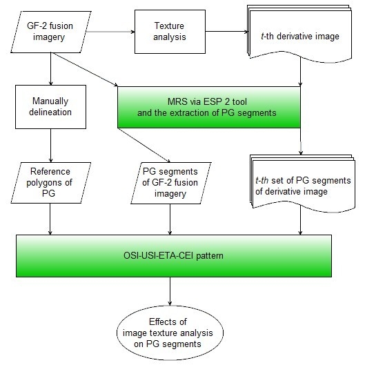
2. Study Area and Data Sets

2.1. Study Area

This study was conducted in Shouguang City, Shandong Province, P.R.China, which is an agricultural region called the "hometown of Chinese vegetable greenhouses" (Figure 1).

The study area (36°44′40″N and 118°49′0″E) was chosen for these reasons: (a) greenhouses are the main local production mode and are developing rapidly in Shouguang City; (b) even though the greenhouses account for nearly half the area in the selected region, they are adjacent to various land cover types such as water, trees, buildings with high reflectance, residences, and barren land, which form a representative common image; and (c) both continuous and scattered greenhouse can be found in the selected region.

2.2. GF-2 Data and Pretreatment

As shown in Figure 1, the GF-2 imagery selected in this study was acquired on April 25, 2016, which is a high-yield period for greenhouse crops [49].

GF-2 is equipped with two high-resolution scanners with 1 m panchromatic and 4 m multispectral, and was launched on August 19, 2014. GF-2 started imaging and transmitting data on August 21, 2014.

Table 1. Payload parameters of GF-2 satellite

Camera	Band No.	Spectral Range (μm)	Spatial Resolution (m)	Swath Width (km)	Side-Looking Ability	Repetition Cycle (Days)
Panchromatic	1	0.45–0.90	1	45 (2 Camera Stitching with)	±35°	5
Multispectral	2	0.45–0.52	4
	3	0.52–0.59
	4	0.63–0.69
	5	0.77–0.89

introduces the payload parameters of the GF-2 satellite [50].

To take full advantage of both panchromatic and multispectral bands, the first pretreatment step is Rational Polynomial Coefficients (RPC) orthorectification, and then image fusion. The Gram-Schmidt Pan Sharpening method in ENVI 5.3 was adopted in this study, and the depth of the resulting fusion image is 16 bits; thus, the greyscale quantization level (GQL) of the GF-2 fusion imagery is 65,536 (2¹⁶).

The computer employed in the experiments had the following specification:

(1)

Processor: Intel^® Core™ i7-8700K CPU @ 3.70GHz (12 CPUs);

(2)

Graphics adapter: NVIDIA^® GeForce^® GTX™ 1080 Ti, 11 GB;

(3)

Memory: SAMSUNG^® DDR4 2400MHz, 2 × 8 GB and SAMSUNG^® DDR4 2400MHz, 2 × 16 GB;

(4)

Hard disk: SAMSUNG^® MZVLW256HEHP-000H1, 256 GB and Seagate^® ST2000DM001-1ER164, 2 TB;

(5)

Operating system: Microsoft^® Windows^® 10 Professional, 64-bit.

2.3. Reference Polygons and Field Validation

To verify extraction results, reference polygons were first manually delineated from the GF-2 fusion image. Polygons that were hard to judge whether or not they represent greenhouses from the image were validated or amended by field investigation. To illustrate, four verification points are demonstrated in Figure 2. Three statistical parameters of the reference polygons were obtained in ArcGIS 10.3 (Esri, Redlands, CA, USA): the number of reference polygons was 151, and the summation area was 1,659,078 m², and the total area of study area was 4,000,000 m².

3. Methodology

A flowchart of experiment design, methods, variables, and indicator system for the evaluation of the effects of texture analysis on PG segments is shown in Figure 3.

3.1. Texture Analysis

Texture is the visual effect caused by spatial variation in tonal quantity over relatively small areas [51], among which the homogeneity and heterogeneity are a pair of coupled features. Even though homogeneity is more frequently employed in texture analysis, we choses the concept of heterogeneity to explain our method and enable understanding. The definition of heterogeneity refers to the distinctly nonuniformity in composition or character (i.e. color, shape, size, texture, etc.)

PG can be more discernible in very high resolution satellite imageries such as Quickbird, Worldview, and GF-2, whereas the heterogeneity is a nonnegligible obstacle when segmenting these images based on GEOBIA. If the heterogeneity of a PG surface can be compressed, a better segmentation result might be derived from the processed image. Considering the nature of heterogeneity in a digital number image, image preprocessing that increases the average operator size (AOS) or decrease the greyscale quantization level (GQL) is the method used to produce derivative images with different heterogeneities in this study.

For an averaging operator [11], the template weighting functions are unity (such as 1/9 in AOS 3 × 3). The goal of averaging is to reduce noise, which is its foundation for compressing the heterogeneity. Averaging is a low-pass filter, since it allows low spatial frequencies to be retained and to suppress high frequency components. The size of an averaging operator is then equivalent to the reciprocal of the bandwidth of the low-pass filter it implements. A larger template, say 11 × 11 or 13 × 13, will remove more noise (high frequencies) but reduce the level of detail.

The GQL size is dependent on the maximum quantization level in a monochromatic image or a single channel of a multichannel image. It can be decreased according to the assigned maximum quantization level and a particular weighted combination of frequencies, which is a redistribution of the greyscale value at each pixel, so that the values can be clustered in a certain range if they are spread over a broad range. As long as GQL decreases, the heterogeneity of each band is compressed.

By increasing AOS or decreasing GQL, information of the pixel’s neighborhood can be effectively used, preceding the MRS. To evaluate the effects of AOS and GQL on MRS segmentation, four increased AOSs (3 × 3, 5 × 5, 7 × 7, and 9 × 9) and three decreased GQLs (128, 64, and 32) were adopted to produce another 19 images based on the initial fusion imagery (GQL initial). Hence, there were 20 input data that were used for segmentation, rather than merely evaluating the segmentation results from the sole data source.

The 19 derivative images were also produced in ENVI 5.3, in which the co-occurrence measures tool can simultaneously change the AOS and GQL of multi-bands among GQL initial, 64, and 32. The derivative images of GQL 128 were produced using the stretch tool, and averaging operations on GQL 128 were conducted using low pass convolution filters, since the co-occurrence measures tool does not support the conversion between GQL initial and GQL 128.

3.2. MRS via ESP 2 Tool

MRS in eCognition is based on the Fractal Net Evolution Approach (FNEA) principle and is widely used for segmentation. It is a region-growing process, and the optimization procedure starts with single-image objects of one pixel and repeatedly merges them in pairs to larger units until an upper threshold is not exceeded locally [8,17,18]. For this purpose, a scale parameter (SP) is proposed to adjust the threshold calculation. Higher values of the scale parameter would result in larger image objects, and smaller values result in smaller image objects. The basic goal of an optimization procedure is to minimize the incorporated heterogeneity at each single merge [8]. If the resulting increase in heterogeneity when fusing two adjacent objects exceeds a threshold determined by the SP, then no further fusion occurs, and the segmentation stops [33]. The SP criteria are defined as a combination of shape and color criteria (color = 1 − shape), whereas shape is interiorly divided as compactness and smoothness criteria; thus, the three parameter values that must be set are SP, shape, and compactness.

ESP 2 is a generic tool for eCognition software that employs local variance (LV) to measure the difference in the MRS under increment scales [22]. When the LV value at a given level (LV_e) is equal to or lower than the value recorded at the previous level (LV_e−1). The level e − 1 is then selected as the OSP for segmentation. Based on this concept, ESP 2 can help derive the dependent SP, whereas shape and compactness can be deduced from the try-and-error experiment within different assessment systems [17,18], which recommend obtaining the SP parameter by fixing the compactness at 0.5 and the testing shape values around 0.3.

Since this study focused on the effect of texture analysis on MRS, the uniform shape and compactness were set to 0.3 and 0.5, respectively. Thus, the OSP was automatically calculated by the ESP 2 tool with the algorithm parameters set as shown in

Table 2. Algorithm parameters and settings in the ESP 2 tool.

Parameter	Value	Parameter	Value
Use of Hierarchy (0 = no; 1 = yes)	1	Starting scale_Level 3	10
Hierarchy: TopDown = 0 or BottomUp = 1?	1	Step size_Level 3	100
Starting scale_Level 1	10	Shape (between 0.1 and 0.9)	0.3
Step size_Level 1	1	Compactness (between 0.1 and 0.9)	0.5
Starting scale_Level 2	10	Produce LV Graph (0 = no; 1 = yes)	1
Step size_Level 2	10	Number of Loops	200

. The Level 1 and its segments in the exported results were adopted for the next step of analysis.

3.3. Extraction of PG Segments

As different derivative images required different samples, features, parameters, or threshold values in automatic extraction, and ensuring good quality is difficult, the greenhouse objects in this study were manually selected by artificial visual interpretation using the single select button on the manual editing toolbar in eCognition 9.0, so that each segmentation object can be as precisely evaluated as possible. Theoretically, manual extraction would have a maximum precision on the criterion of geometric accuracy, but this is only credible for the criterion of the area, since, in other methods, the commission area also has a probability of offsetting the omissions while the geometric error can only be accumulated.

The principle used to assign an object as a greenhouse is when the proportion of greenhouse area is more than 60% [24] and the feature of other categories is negligible from visual analysis. Otherwise, the object’s feature is deemed to be unusable to extract the greenhouse contained within, which would be evaluated as omission error in follow-up work.

After exporting from eCognition 9.0, two statistical parameters of the extracted PG segments were obtained in ArcGIS 10.3: number of PG segments and summation area.

3.4. Establishment of OSI-USI-ETA-CEI Pattern

3.4.1. Case Study and Variable Definition

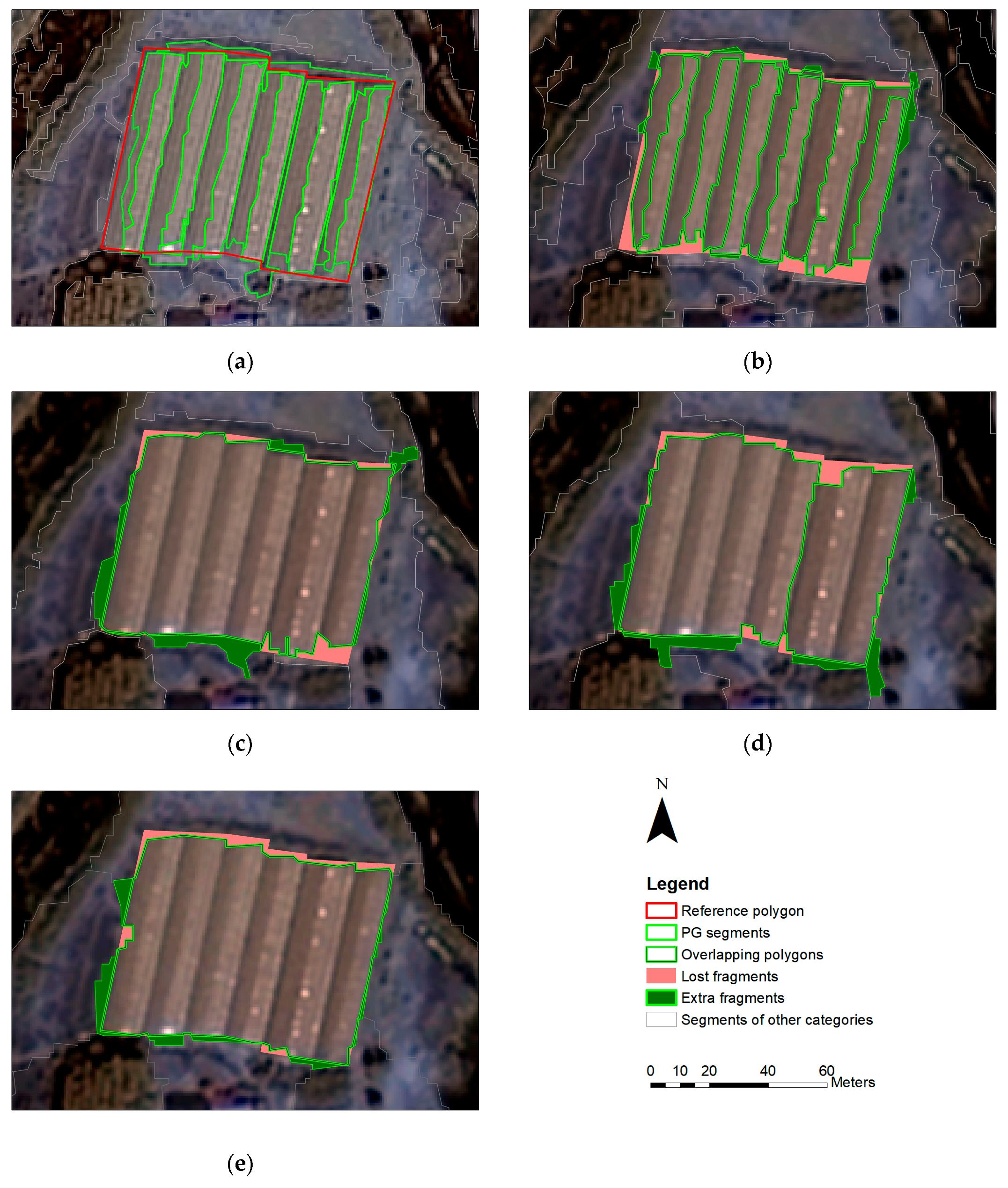
To better understand the problems in PG segmentation, the definitions of variables, and the establishment of OSI-USI-ETA-CEI pattern, five cases of PG segments that were extracted from initial GF-2 fusion imagery and four derivative images are demonstrated in Figure 4, and all images were segmented under their optimal scale parameter provided by the ESP 2 tool. Notably, these cases cannot represent the segmentation quality of a whole image.

Without decreasing the GQL, the degree of over-segmentation of the PG segments that were extracted from the initial GF-2 fusion imagery (Figure 4a) or images derived from the treatment of AOS 3 × 3 (Figure 4b) are much worse than those extracted from other derivative images (Figure 4c–e), since the dark and the sunny sides of the PG in the two images are segmented as different parts, making it hard to delineate the PGs’ boundaries, which is not convenient for subsequent feature recognition and extraction.

Apart from the number of PG segments, the number and area of the fragments (the smaller polygons that are partitioned jointly by reference polygons and PG segments) are also need to be explored in depth.

To parameterize the relationship between the reference polygons and PG segments, four quantity-based variables, seven area-based variables and their assemblies were defined in

Table 3. Four quantity-based variables, seven area-based variables and their assemblies.

Variable	Definition
m	total number of reference polygons
v	total number of PG segments
n	number of reference polygons that have no PG segments overlapping with them, n ≤ m
ux	x-th number of corresponding segments found for one single reference geometry, x ∈ (0, m − n] [45]
ri	i-th reference polygon of assembly R; R indicates the real area of PG, i ∈ (0, m]
sj	j-th extracted PG segment of assembly S; S indicates the extraction area of PG, j ∈ (0, v]
ok	k-th polygon of assembly O; O indicates the overlapping area between R and S, O = R ∩ S
bsh	h-th element of Biggest Segments (BS); BS is the assembly of PG segments representing the biggest overlapping polygon within its corresponding reference polygon, indicating the total area of biggest segments, BS ⊆ S
boh	h-th element of Biggest Overlaps (BO); BO is the assembly of overlapping polygons where each is partitioned by every bsh and its corresponding reference polygon, indicating the total area of biggest overlaps, BO ⊆ O
lfp	p-th element of Lost Fragments (LF); LF is the assembly of fragments where each is part of R and also part of a segment that cannot represent PG (fragments in R but outside of O, which are shown in coral red in Figure 4), LF indicates the total area of lost fragments [24]
efq	q-th element of Extra Fragments (EF); EF is the assembly of fragments where each is part of S but not part of R itself (fragments in S but outside O, shown in dark green in Figure 4), EF indicates the total area of extra fragments [24]

:

It is generally thought that a high-quality image segmentation should result in a minimum amount of over- and under-segmentation, and different area-based or number-based indicators have been designed based on selected samples and their corresponding reference polygons [14,24,39,41,42,43,45,52], which we rewrote using variables defined above for comparison, as shown in

Table 4. Different area-based or number-based indicators of over- and under-segmentation.

Year	Reference	Over-Segmentation	Under-Segmentation
2002	Lucieer et al. [38]	$\frac{r_i-b{s}_h}{r_i}$ > 0	$\frac{r_i-b{s}_h}{r_i}$ < 0
2007	Möller et al. [39]	$\frac{o_k}{r_i}$	$\frac{o_k}{s_j}$
2010	Clinton et al. [40]	$1-\frac{o_k}{r_i}$	$1-\frac{o_k}{s_j}$
2010	Persello et al. [41]	$1-\frac{b{o}_h}{r_i}$	$1-\frac{b{o}_h}{s_j}$
2010	Marpu et al. [24]	$\frac{b{o}_h}{r_i}$	$\frac{{\mathrm{lf}}_p}{r_i}$, $\frac{{\mathit{ef}}_q}{r_i}$
2012	Liu et al. [42]	$\mathrm{NSR}=\frac{\left|m-v\right|}{m}$	$\mathrm{PSE}=\frac{EF}{R}$
2016	Novelli et al. [45]	${\mathrm{NSR}}_{\mathrm{new}}=\frac{\left|m-v-n\times \max \left(u_x\right)\right|}{m-n}$	${\mathrm{PSE}}_{\mathrm{new}}=\frac{EF+n\times \max ({\mathit{ef}}_q)}{{\displaystyle {\sum }_{i=1}^{m-n}{r}_i}}$

.

Some feature similarity-based, location-based or distance-based [41,46] methods are available for measuring the quality of segmentation, but these methods only work when segments have an approximately one-to-one relationship with the reference polygons, whereas the segmentation results of continuous greenhouses always have the relationship with the reference of poly-to-one.

The OSI-USI-ETA-CEI pattern is based on the reference polygons that were manually delineated in Section 2.3. and the PG segments extracted in Section 3.3. The method is designed for evaluating the segmentation quality of PG segments from images with different heterogeneities. In short, OSI denotes the extent to which the number of PG segments may affect the USI and ETA, USI indicates the absolute geometric error of PG segments, ETA indicates the discrepancy in the total area between PG segments and reference polygons, and CEI indicates the composite error.

3.4.2. Over-Segmentation Index (OSI)

Segmentation results that are over-segmented are more likely to cause omission and commission errors in follow-up classification because the number and some feature values (like mean value) of both the interested and non-interested objects that are over-segmented would range widely compared with those that are not over-segmented. An extreme example of this is when an image is segmented on the pixel level. Even though it is much easier to compare the number rather than other feature values for two assemblies of polygons, indicators that compare the number of reference polygons with segments [17,18,42,43,44,45] and that compare the area of a reference polygon with its biggest corresponding segment [24,38,53] were both designed or applied in over-segmentation analysis. However, these criteria are designed for pursuing perfect segmentation that is similar to manually delineated reference polygons, which is not suitable for evaluating the segments of continuous PGs since drawing those reference polygons is different from segmenting an image. Reference polygons prefer to draw the outline of a single or continuous greenhouse rather than divide pixels with different grey levels, whereas segmentation prefers the latter, especially when some pixels’ material or Bidirectional Reflectance Distribution Function (BRDF) varies significantly from their surrounding pixels. To manually draw the outline of continuous greenhouses is so subjective that it is hard to determine the size of a reference polygon as well as the total number of reference polygons, i.e., no wonderful polygons can be used to define whether a segmentation is over-segmented or not. A similar view was reported by Zhang et al. [30]. Thus, continuous greenhouse extraction in high-resolution imagery does not require a similar segment number compared to the manual reference polygons, nor accordant outlines or even skeletons (Figure 4). However, we should consider counting the segment numbers in the initial fusion imagery as an effective reference to assess over-segmentation instead, since the high heterogeneity among greenhouse pixels in an initial fusion image tends to lead to the worst over-segmenting result compared with derivative images with lower heterogeneity. Therefore, the segment numbers of the initial fusion imagery under its OSP using ESP 2 can be regarded as ancillary data of reference polygons in Section 2.3. The ancillary data provides a numerical reference and the manually delineated polygons provides a geometric reference.

Synthesizing the situation stated above, over-segmentation of PG segments is indicated by a new OSI in this study, which is a relative value calculated by Equation (1):

$$\mathrm{OSI}=\frac{v}{v_1}$$

(1)

where v denotes the number of extracted PG segments when the corresponding image is under the optimal segmentation using ESP 2 tool, v₁ denotes the number of PG segments extracted from the initial GF-2 fusion image, and v_t+1 denotes the number of PG segments extracted from the t-th derivative image. A higher OSI indicates a larger error of over-segmentation.

3.4.3. Under-Segmentation Index (USI)

When an image is over-segmented, it is still possible to construct the object, but when an image is under-segmented, the object may not be recovered [24]. Under-segmentation is more worthwhile to be exactly evaluated.

From Figure 4, both lost and extra fragments are shown to have many members with very tiny areas, and the boundaries of the reference polygons usually have fewer polylines than that of PG segments. The number of lost and extra fragments are not only caused by geometric errors but also changed by how we draw the outline of single or continuous greenhouses, so it is not appropriate to neither count the number nor calculate the mean value of those fragments [24] when evaluating the geometric errors of continuous greenhouses.

In general, the area of extra-segments are parts of under-segmentation error according to some studies (Table 4), as the PG segments should slice those pixels that are not representing a PG. However, lost fragments can be considered as a result of under-segmentation of those segments that do not contain enough PG pixels, i.e., the lost fragments can be regarded as the extra fragments of another category (Figure 4). Therefore, it is necessary to adequately evaluate both the LF and EF error rather than to consider only one and then combine the two errors into a single index (USI) to indicate the intension of under-segmentation of PG segments. The theoretical value should range between zero and one. The index can be calculated as:

$$\mathrm{USI}=\frac{LF+EF}{R}$$

(2)

where LF, EF, and R are the total area of lost fragments, extra fragments, and the real area of PG, respectively. A higher USI indicates a larger under-segmentation error.

3.4.4. Error Index of Total Area (ETA)

Lost and extra fragments have an opposite influence on the final area of extraction even though both directly contribute to the under-segmentation. Although area-based measures were discussed in Clinton et al. [40] and some new measures based on area were designed after that [24,42,46], these sample-based studies only focused on the proportion of the omission or commission area in a segmentation, but the percentage of the difference in the total area between segmentation results and corresponding reference polygons seems to be ignored, which should be fully considered when evaluating the precision of the total area of extraction and the consequence of under-segmentation. Thus, the Error Index of Total Area (ETA) can be used to indicate the discrepancy, which can be calculated by:

$$\mathrm{ETA}=\frac{\left|S-R\right|}{R}=\frac{\left|EF-LF\right|}{R}$$

(3)

where S denotes the summation area of extracted PG segments when corresponding image is under the optimal segmentation using the ESP 2 tool, S₁ denotes the summation area of PG segments extracted from the initial GF-2 fusion image, and S_t+1 denotes the summation area of PG segments extracted from the t-th derivative image. A higher ETA value indicates a larger total area error.

3.4.5. Composite Error Index (CEI)

In general, the more the PG segments are over-segmented, the larger the omission and commission error produced indirectly in automatic classification or extraction. Under-segmentation causes geometric errors and directly leads to an area difference from the reference. Given this consideration, a new CEI is presented in Equation (4) to consider the composite error of segmentation results when comparing to a set of reference polygons:

$$\mathrm{CEI}=\lambda \times \mathrm{OSI}+\mathrm{USI}+\mathrm{ETA}$$

(4)

where λ is a possible weight used to rescale the value of quantity-based OSI so that the indicator will not overwhelm the value of area-based USI and ETA; thus, the OSI multiplied by λ denotes the indirect influence of the number of PG segments on extraction in CEI.

When omission or commission segments in an extraction are generated due to over-segmenting, their geometric error and area difference from the real value (indicated by USI and ETA, respectively) couple on the extraction. Thus, the value of λ in this study is defined as the sum of USI and ETA as:

$$\lambda =\mathrm{USI}+\mathrm{ETA}$$

(5)

4. Results

4.1. Derivative Images with Different Heterogeneities

We provide two images (Figure 5) as examples to show the visual disparity of different heterogeneities. Even though there is no significant difference at first sight, some subtle distinctions can be found from the white roof (in red frame), and the texture in image that derived from the treatment of GQL 64 and AOS 3 × 3 is more distinct than in initial GF-2 fusion imagery. Details emerge in the images as long as they are segmented (Figure 6).

4.2. PG Segments in Images with Different Heterogeneities

Seven sets of PG segments are shown in Figure 6 as examples to demonstrate the visual disparity. The number of PG segments extracted from initial fusion imagery is outdistancing the other situations as well as reference polygons. Another significant difference is the number of segments of the white roof (in red frame). In Figure 6a–c, the roof’s boundary is hard to distinguish from the thumbnails, while the other examples are much better. The boundaries of the PG segments in Figure 6c,d are more orderly both horizontally and vertically, which conforms to the outlines of the greenhouses, whereas the segmentation results in Figure 6e–g irregularly delineate the greenhouses.

Apart from the examples in Figure 6, the indicator values of each set of PG segments that were extracted from different images are shown in

Table 5. Indicator values of each set of PG segments that were extracted from different images.

GQL	AOS	OSP	v	S (m2)	LF (m2)	EF (m2)	OSI	USI	ETA	CEI	DIF
initial	none	81	3007	1,690,287	86,211	117,420	1.000	0.123	0.019	0.283	0.000
	3 × 3	103	1737	1,659,104	109,546	109,572	0.578	0.132	0.000	0.208	−0.075
	5 × 5	161	711	1,733,075	89,339	163,336	0.236	0.152	0.045	0.243	−0.040
	7 × 7	197	446	1,710,681	114,154	165,757	0.148	0.169	0.031	0.229	−0.054
	9 × 9	151	507	1,693,593	122,930	157,805	0.169	0.169	0.021	0.222	−0.061
128	none	82	808	1,700,510	102,356	143,788	0.269	0.148	0.025	0.220	−0.063
	3 × 3	94	561	1,660,182	128,221	129,325	0.187	0.155	0.001	0.185	−0.098
	5 × 5	109	380	1,679,966	133,606	154,494	0.126	0.174	0.013	0.210	−0.073
	7 × 7	100	400	1,689,608	123,859	154,389	0.133	0.168	0.018	0.211	−0.072
	9 × 9	115	267	1,703,666	117,728	162,316	0.089	0.169	0.027	0.213	−0.070
64	none	50	457	1,781,987	87,601	210,510	0.152	0.180	0.074	0.292	0.009
	3 × 3	56	352	1,796,653	90,983	228,558	0.117	0.193	0.083	0.308	0.025
	5 × 5	64	255	1,827,083	83,023	251,028	0.085	0.201	0.101	0.328	0.045
	7 × 7	67	250	1,870,392	72,295	283,609	0.083	0.215	0.127	0.370	0.087
	9 × 9	82	171	1,903,843	81,584	326,349	0.057	0.246	0.148	0.416	0.133
32	none	31	821	1,738,822	103,795	183,539	0.273	0.173	0.048	0.282	−0.001
	3 × 3	39	527	1,793,144	96,658	230,724	0.175	0.197	0.081	0.327	0.044
	5 × 5	46	355	1,773,550	130,505	244,977	0.118	0.226	0.069	0.330	0.047
	7 × 7	49	361	1,792,180	119,801	252,903	0.120	0.225	0.080	0.341	0.058
	9 × 9	46	379	1,802,023	110,171	253,116	0.126	0.219	0.086	0.344	0.061

, while the summation area of reference polygons (R) was 1,659,078 m², and OSP is the optimal scale parameter calculated by the ESP 2 tool with fixed shape of 0.3 and compactness of 0.5. We use DIF denotes the value of CEI of each set of PG segments minus that of PG segments of the initial fusion imagery.

The experiment was designed to find the optimal set of GQL and AOS, which could result in optimum PG segments for the extraction. PG segments in derivative image with the treatment of GQL 128 and AOS 3 × 3 has the lowest CEI, which is consistent with visual analysis in Section 3.

4.3. Effects of Image Texture Analysis on PG Segments

4.3.1. Effects of Increasing AOS on PG Segments

Images under four kinds of GQLs can be employed to process by four AOSs, so we could evaluate the effects of increasing AOS on PG Segments as Figure 7 and Figure 8 shown.

With the increase in AOS (Figure 7), both the sum of LF and EF (related to USI) and the distances between them (related to ETA) have relatively low values under the treatments of GQL initial and GQL 128 than that of GQL 64 and GQL 32. Variation of LF and EF is the foundation to understand the value of USI and ETA, while the sum of USI and ETA is main source of CEI (Figure 8).

For GQL initial and GQL 128, the AOS 3 × 3 setup can let the values of ETA and CEI reach their minimum simultaneously, and significantly decrease the value of OSI, whereas USI increases somewhat.

For GQL 64 and GQL 32, the increase in AOS lead to the increase in CEI, which was not expected.

For each kind of GQL, the increase in AOS lead to opposite change trends of USI and OSI, whereas CEI had the same with ETA. The curves under GQL 128 are smoother and steadier than other GQLs with increasing AOS.

4.3.2. Effects of Decreasing GQL on PG Segments

Five AOS setups were used to evaluate the effects of decreasing GQL on PG Segments as shown in Figure 9 and Figure 10.

Similar to Figure 7, Figure 9 demonstrates the superiority of GQL initial and GQL 128 on both the sum of LF and EF (related to USI) and the distances between them (related to ETA), which shows the lower omission and commission errors of PG segments than GQL 64 and GQL 32.

From Figure 10, the treatment of GQL 128 has the lowest CEI values under each setup of AOS compared to other GQLs, among of which AOS 3 × 3 produced the minimum value.

4.3.3. Combined Effects of AOS and GQL on PG Segments

Compared with the initial fusion imagery, the increase in AOS and the decrease in GQL can reduce the influence of over-segmentation but can also increase the error of both under-segmentation and the extraction area. An interaction of the effects occurs among OSI, USI, and ETA, all of which synthetically decide the CEI.

After the treatment of different AOSs on GQL initial and GQL 128, the CEI was reduced by 4.0 to 9.8% compared to the initial fusion imagery, whereas the treatment of different AOSs on GQL 64 and GQL 32 increase the CEI by 0.9 to 13.0%, except that of GQL 32 without an averaging operator, which was very close to the initial fusion imagery with only a 0.1% reduction.

Thus, the optimum texture analysis setup for GF-2 fusion imagery is GQL 128 and AOS 3 × 3, since the PG segments of the derivate image can reduce the CEI by 9.8% than PG segments of the GF-2 fusion imagery.

5. Discussion

Since the segmentation results from the initial fusion image are highly fragmented compared with the boundary of real-world entities, compressing the heterogeneity of adjacent pixels before segment was notable. To improve the PG segments derived from eCognition, the innovation of our method is that we evaluate the effects of texture analysis on PG segments using OSI-USI-ETA-CEI pattern, based on the nature of segmentation and heterogeneity in a digital number image.

5.1. Evaluation Problems

Several problems need to be considered when measurement methods are used for the evaluation of PG segments.

First, the confusion matrix is a common method for evaluation or verification, but in object-based extraction, a problem occurs for each segmented object: omission and commission errors may coexist compared to the reference polygon. Thus, the extraction result cannot be accurately evaluated by choosing those segmented objects with an inaccurate boundary as the true values [19,20]. Each greenhouse object’s omission and commission errors should be considered on the pixel-based rather than the object-based level.

If the specified proportion of a greenhouse that is adopted to define a segment as a PG increases or reduces, the percentage of LF and EF would change either [24].

As a non-negligible indicator, the difference in the area between the extraction results and the reference polygons must also be evaluated quantitatively.

5.2. Comparison with Related Evaluation Research

Several pointed discussions in Section 3.4. theoretically explained why the OSI-USI-ETA-CEI method differs from existing indexes, which is summarized in

Table 6. Comparing the OSI-USI-ETA-CEI pattern with related evaluation research.

Proposed Pattern	Comparation with Related Evaluation Research
OSI	Calculated by the ratio of the number of PG segments of derivate image to the number of PG segments of initial fusion imagery, instead of ignoring the impact of the number, or assuming the delineated polygons have a dependable quantity
USI	Calculated by the proportion of area of lost and extra fragments together as a consequence of under-segmentation, instead of calculating only one of them or separately
ETA	Considers the difference in area between extraction results and reference polygons
CEI	Rescale the OSI by geometry and area discrepancy first and then simply sum the rescaled OSI with USI and ETA up, instead of calculating the Euclidean Distance of indicator values

. Notably, the existing indexes are designed based on scattered reference polygons and the corresponding overlapped PG segments, whereas the OSI-USI-ETA-CEI method in this study was built on the whole image.

Even though the effect of different shape and compactness values on PG segments are not discussed in this study, we selected them on the basis of Aguilar et al. [17,18], which considered ESP 2 to be an effective tool on PG segmentation. Aguilar et al. [17] evaluated the effects of shape and compactness on the quality of PG segments by the ED2 in Equation (6), and Aguilar et al. [18] compared the PG segments derived from multispectral, panchromatic, and atmospheric correctional multispectral orthoimages under different shape and compactness values by the modified ED2 in Equation (7):

$$\mathrm{ED}2=\sqrt{{\mathrm{PSE}}^2+{\mathrm{NSR}}^2}$$

(6)

$$modified\mathrm{ED}2=\sqrt{{\mathrm{PSE}}_{\mathrm{new}}^2+{\mathrm{NSR}}_{\mathrm{new}}^2}$$

(7)

where PSE, NSR, PES_new, and NSR_new were defined in Section 3.4.1.

The ED2, modified ED2 and CEI are all evaluation methods based on both numeral and areal indicators. Since the ED2 has a similar principle to the modified ED2 and is more computable than that, we use the PSE-NSR-ED2 method contrasted with the OSI-USI-ETA-CEI pattern by numerical and visualized analysis to support our availability.

The best texture analysis setup for GF-2 fusion imagery according to ED2 value is GQL 64 and AOS 9 × 9, which was judged as the worst one by USI, ETA, CEI and even PSE. Furthermore, the ED2 almost determined by the NSR (

Table 7. Values of PSE, NSR, and ED2 of each set of PG segments under different GQL and AOS.

GQL	AOS	PSE	NSR	ED2	GQL	AOS	PSE	NSR	ED2
Initial	none	0.071	18.914	18.914	64	none	0.127	2.026	2.030
	3 × 3	0.066	10.503	10.504		3 × 3	0.138	1.331	1.338
	5 × 5	0.098	3.709	3.710		5 × 5	0.151	0.689	0.705
	7 × 7	0.100	1.954	1.956		7 × 7	0.171	0.656	0.678
	9 × 9	0.095	2.358	2.360		9 × 9	0.197	0.132	0.237
128	none	0.087	4.351	4.352	32	none	0.111	4.437	4.438
	3 × 3	0.078	2.715	2.716		3 × 3	0.139	2.490	2.494
	5 × 5	0.093	1.517	1.519		5 × 5	0.148	1.351	1.359
	7 × 7	0.093	1.649	1.652		7 × 7	0.152	1.391	1.399
	9 × 9	0.098	0.768	0.774		9 × 9	0.153	1.510	1.518

and Figure 11) shows that ED2 is not suit to evaluate the quality of segmentation results in this study.

Therefore, the drawbacks of the ED2 [42] are: (1) equated the attribute of numerical indicator with that of areal indicator; (2) gave the larger indicator a bigger weight than the smaller one in calculation. The modified ED2 does this as well, which is not expected to happen when compositing the numerical and areal indicators.

Although the PSE-NSR-ED2 method loses its efficacy in this study, it did work in several studies [17,42,43,44]. A possible reason is the heterogeneity of the images of their study areas was not as high as that of the GF-2 fusion data in this study [17].

5.3. Next Steps

Although the experiments are all based on MRS in eCognition, the proposed methods are presented in a general sense and may helpful for practitioners who suffer from segmentation issues in GEOBIA.

The drawback of the proposed method is the number of PG segments relies on the validity of the ESP 2 tool and the PG segments must be obtained by manual selection. Thus, other effective segmentation schemes or automatic extraction methods are needed for experimentation with the method in the future.

We only analyzed the effects of two preprocessing operations (increasing AOS and decreasing GQL) on PG segments, whereas the influence of atmospheric correction on PG segments was evaluated by Aguilar et al. [18], but different methods or tools to change the heterogeneity of input imagery are available, such as median filter, Gaussian averaging operator, Region-Scalable Fitting (RSF) model, and the Laplacian of Gaussian (LoG) operator [11,13].

Since segmentation results are highly scene-dependent, the investigation should also be applied to other scenes and data sources in future studies.

6. Conclusions

This study was designed to examine the ability of extracting greenhouses from GF-2 imagery. To complete the process, compressing the heterogeneity of the initial fusion image was designed to effectively use the texture analysis and improve the MRS, and a new OSI-USI-ETA-CEI pattern was proposed to evaluate the effects of texture analysis on PG segments.

Although this work should be only considered as an initial approach, the following conclusions are drawn:

(1)

Appropriate texture analysis applied to a fusion image can change its heterogeneity effectively for better segmentation.

(2)

When shape and compactness are fixed at 0.3 and 0.5 respectively, the optimum treatment of GF-2 fusion imagery prior to segmenting the plastic greenhouses using ESP 2 tool is compresses the GQL to 128 and uses the AOS 3 × 3 setup, which reduces the CEI by 9.8% compared with the initial fusion imagery in this study.

(3)

The proposed OSI-USI-ETA-CEI pattern can be applied to evaluate the effects of image processing on the quality of PG segments, which is more accurate but requires a higher workload than the PSE-NSR-ED2 method.

References

1. Ma, L.; Li, M.C.; Ma, X.X.; Cheng, L.; Du, P.J.; Liu, Y.X. A review of supervised object-based land-cover image classification. ISPRS J. Photogramm. Remote Sens. 2017, 130, 277–293. [Google Scholar] [CrossRef]
2. Levinshtein, A.; Stere, A.; Kutulakos, K.N.; Fleet, D.J.; Dickinson, S.J.; Siddiqi, K. TurboPixels: Fast superpixels using geometric flows. IEEE Trans. Pattern Anal. Mach. Intell. 2009, 31, 2290–2297. [Google Scholar] [CrossRef] [PubMed]
3. Schick, A.; Fischer, M.; Stiefelhagen, R. An evaluation of the compactness of superpixels. Pattern Recognit. Lett. 2014, 43, 71–80. [Google Scholar] [CrossRef]
4. Tian, X.; Jiao, L.; Yi, L.; Guo, K.; Zhang, X. The image segmentation based on optimized spatial feature of superpixel. J. Vis. Commun. Image Represent. 2015, 26, 146–160. [Google Scholar] [CrossRef]
5. Stutz, D.; Hermans, A.; Leibe, B. Superpixels: An evaluation of the state-of-the-art. Comput. Vis. Image Underst. 2018, 166, 1–27. [Google Scholar] [CrossRef] [Green Version]
6. Cousty, J.; Bertrand, G.; Najman, L.; Couprie, M. Watershed cuts: Thinnings, shortest path forests, and topological watersheds. IEEE Trans. Pattern Anal. Mach. Intell. 2010, 32, 925–939. [Google Scholar] [CrossRef]
7. Ciecholewski, M. Automated coronal hole segmentation from Solar EUV Images using the watershed transform. J. Vis. Commun. Image Represent. 2015, 33, 203–218. [Google Scholar] [CrossRef]
8. Baatz, M.; Schäpe, A. Multiresolution segmentation: An optimization approach for high quality multi-scale image segmentation. In Angewandte Geographische Informationsverarbeitung; Herbert Wichmann Verlag: Heidelberg, Germany, 2000; pp. 12–23. [Google Scholar]
9. Tian, J.; Chen, D.M. Optimization in multi-scale segmentation of high-resolution satellite images for artificial feature recognition. Int. J. Remote Sens. 2007, 28, 4625–4644. [Google Scholar] [CrossRef]
10. Trimble. eCognition Developer 9.3 Reference Book; Trimble Germany GmbH: Munich, Germany, 2017. [Google Scholar]
11. Nixon, M.S.; Aguado, A.S. Feature Extraction & Image Processing for Computer Vision, 3rd ed.; Elservier and Pte Ltd.: Singapore, 2012. [Google Scholar]
12. Balla-Arabé, S.; Gao, X. Geometric active curve for selective entropy optimization. Neurocomputing 2014, 139, 65–76. [Google Scholar] [CrossRef]
13. Ding, K.; Xiao, L.; Weng, G. Active contours driven by region-scalable fitting and optimized Laplacian of Gaussian energy for image segmentation. Signal Process. 2017, 134, 224–233. [Google Scholar] [CrossRef]
14. Neubert, M.; Herold, H.; Meinel, G. Assessing Image Segmentation Quality—Concepts, Methods and Application; Springer: Berlin, Germany, 2008. [Google Scholar]
15. Neubert, M.; Herold, H. Assessment of remote sensing image segmentation quality. In Proceedings of the GEOBIA, Calgary, AB, Canada, 6–7 August 2008; p. 5. [Google Scholar]
16. Blaschke, T. Object based image analysis for remote sensing. ISPRS J. Photogramm. Remote Sens. 2010, 65, 2–16. [Google Scholar] [CrossRef] [Green Version]
17. Aguilar, M.A.; Aguilar, F.J.; García Lorca, A.; Guirado, E.; Betlej, M.; Cichon, P.; Nemmaoui, A.; Vallario, A.; Parente, C. Assessment of Multiresolution Segmentation for Extracting Greenhouses from Worldview-2 Imagery. ISPRS Int. Arch. Photogramm. Remote Sens. Spat. Inf. Sci. 2016, XLI-B7, 145–152. [Google Scholar] [CrossRef]
18. Aguilar, M.A.; Novelli, A.; Nemamoui, A.; Aguilar, F.J.; García Lorca, A.; González-Yebra, Ó. Optimizing Multiresolution Segmentation for Extracting Plastic Greenhouses from WorldView-3 Imagery. In Proceedings of the Intelligent Interactive Multimedia Systems and Services, Gold Coast, Australia, 20–22 May 2017; pp. 31–40. [Google Scholar]
19. Coslu, M.; Sonmez, N.K.; Koc-San, D. Object-Based Greenhouse Classification from High Resolution Satellite Imagery: A Case Study Antalya-Turkey. ISPRS Int. Arch. Photogramm. Remote Sens. Spat. Inf. Sci. 2016, XLI-B7, 183–187. [Google Scholar] [CrossRef]
20. Wu, C.; Deng, J.; Wang, K.; Ma, L.; Shah, T.A.R. Object-based classification approach for greenhouse mapping using Landsat-8 imagery. Int. J. Agric. Biol. Eng. 2016, 9, 79–88. [Google Scholar]
21. Drǎguţ, L.; Tiede, D.; Levick, S.R. ESP: A tool to estimate scale parameter for multiresolution image segmentation of remotely sensed data. Int. J. Geogr. Inf. Sci. 2010, 24, 859–871. [Google Scholar] [CrossRef]
22. Dragut, L.; Csillik, O.; Eisank, C.; Tiede, D. Automated parameterisation for multi-scale image segmentation on multiple layers. ISPRS J Photogramm Remote Sens 2014, 88, 119–127. [Google Scholar] [CrossRef] [Green Version]
23. d’Oleire-Oltmanns, S.; Tiede, D. Specific target objects—Specific scale levels? Application of the estimation of scale parameter 2 (ESP 2) tool for the identification of scale levels for distinct target objects. South-East. Eur. J. Earth Obs. Geomat. 2014, 3, 580–583. [Google Scholar]
24. Marpu, P.R.; Neubert, M.; Herold, H.; Niemeyer, I. Enhanced evaluation of image segmentation results. J. Spat. Sci. 2010, 55, 55–68. [Google Scholar] [CrossRef]
25. Su, W.; Li, J.; Chen, Y.; Liu, Z.; Zhang, J.; Low, T.M.; Suppiah, I.; Hashim, S.A.M. Textural and local spatial statistics for the object-oriented classification of urban areas using high resolution imagery. Int. J. Remote Sens. 2008, 29, 3105–3117. [Google Scholar] [CrossRef]
26. Agüera, F.; Aguilar, F.J.; Aguilar, M.A. Using texture analysis to improve per-pixel classification of very high resolution images for mapping plastic greenhouses. Isprs J. Photogramm. Remote Sens. 2008, 63, 635–646. [Google Scholar] [CrossRef]
27. Hasituya; Chen, Z.; Wang, L.; Wu, W.; Jiang, Z.; Li, H. Monitoring Plastic-Mulched Farmland by Landsat-8 OLI Imagery Using Spectral and Textural Features. Remote Sens. 2016, 8, 353. [Google Scholar] [CrossRef]
28. Haralick, R.M.; Shanmugam, K.; Dinstein, I. Texture features for image classifications. IEEE Trans. Syst. Man Cybern. 1973, 3, 610–621. [Google Scholar] [CrossRef]
29. Aguilar, M.A.; Nemmaoui, A.; Novelli, A.; Aguilar, F.J.; García Lorca, A. Object-Based Greenhouse Mapping Using Very High Resolution Satellite Data and Landsat 8 Time Series. Remote Sens. 2016, 8, 513. [Google Scholar] [CrossRef]
30. Zhang, H.; Fritts, J.E.; Goldman, S.A. Image segmentation evaluation: A survey of unsupervised methods. Comput. Vis. Image Underst. 2008, 110, 260–280. [Google Scholar] [CrossRef] [Green Version]
31. Zhang, X.; Xiao, P.; Feng, X. An Unsupervised Evaluation Method for Remotely Sensed Imagery Segmentation. IEEE Geosci. Remote Sens. Lett. 2012, 9, 156–160. [Google Scholar] [CrossRef]
32. Gao, H.; Tang, Y.; Jing, L.; Li, H.; Ding, H. A Novel Unsupervised Segmentation Quality Evaluation Method for Remote Sensing Images. Sensor 2017, 17, 2427. [Google Scholar] [CrossRef]
33. Wang, Y.; Qi, Q.; Liu, Y. Unsupervised Segmentation Evaluation Using Area-Weighted Variance and Jeffries-Matusita Distance for Remote Sensing Images. Remote Sens. 2018, 10, 1193. [Google Scholar] [CrossRef]
34. Yang, L.; Albregtsen, F.; Lønnestad, T.; Grøttum, P. A supervised approach to the evaluation of image segmentation methods. Comput. Anal. Images Patterns 1995, 759–765. [Google Scholar]
35. Zhang, Y.J. A survey on evaluation methods for image segmentation. Pattern Recognit. 1996, 29, 1335–1346. [Google Scholar] [CrossRef]
36. Chabrier, S.; Laurent, H.; Emile, B.; Rosenberger, C.; Marche, P. A comparative study of supervised evaluation criteria for image segmentation. In Proceedings of the EUSIPCO, Vienna, Austria, 6–10 September 2004; pp. 1143–1146. [Google Scholar]
37. Correia, P.; Pereira, F. Objective evaluation of relative segmentation. In Proceedings of the International Conference on Image Processing, Vancouver, BC, Canada, 10–13 September 2000; pp. 308–311. [Google Scholar]
38. Lucieer, A.; Stein, A. Existential uncertainty of spatial objects segmented from satellite sensor imagery. IEEE Trans. Geosci. Remote Sens. 2002, 40, 2518–2521. [Google Scholar] [CrossRef]
39. Möller, M.; Lymburner, L.; Volk, M. The comparison index: A tool for assessing the accuracy of image segmentation. Int. J. Appl. Earth Obs. Geoinf. 2007, 9, 311–321. [Google Scholar] [CrossRef]
40. Clinton, N.; Holt, A.; Scarborough, J.; Yan, L.; Gong, P. Accuracy Assessment Measures for Object-based Image Segmentation Goodness. Photogramm. Eng. Remote Sens. 2010, 76, 289–299. [Google Scholar] [CrossRef]
41. Persello, C.; Bruzzone, L. A Novel Protocol for Accuracy Assessment in Classification of Very High Resolution Images. IEEE Trans. Geosci. Remote Sens. 2010, 48, 1232–1244. [Google Scholar] [CrossRef]
42. Liu, Y.; Bian, L.; Meng, Y.; Wang, H.; Zhang, S.; Yang, Y.; Shao, X.; Wang, B. Discrepancy measures for selecting optimal combination of parameter values in object-based image analysis. ISPRS J. Photogramm. Remote Sens. 2012, 68, 144–156. [Google Scholar] [CrossRef]
43. Liu, Y.; Zhang, Y.D.; Huang, Z.; Wang, M.M.; Yang, D.; Ma, H.M.; Zhang, Y.X.; Li, Y.F.; Li, H.W.; Hu, X.G. Segmentation optimization via recognition of the PSE-NSR-ED2 patterns along with the scale parameter in object-based image analysis. In Proceedings of the GEOBIA 2016: Solutions and Synergies, Enschede, The Netherlands, 14–16 September 2016. [Google Scholar]
44. Gao, M.; Qunou, J.; Yiyang, Z.; Wentao, Y.; Mingchang, S. Comparison of plastic greenhouse extraction method based on GF-2 remote-sensing imagery. J. China Agric. Univ. 2018, 23, 125–134. [Google Scholar]
45. Novelli, A.; Aguilar, M.A.; Nemmaoui, A.; Aguilar, F.J.; Tarantino, E. Performance evaluation of object based greenhouse detection from Sentinel-2 MSI and Landsat 8 OLI data: A case study from Almería (Spain). Int. J. Appl. Earth Obs. Geoinf. 2016, 52, 403–411. [Google Scholar] [CrossRef]
46. Cai, L.; Shi, W.; Miao, Z.; Hao, M. Accuracy Assessment Measures for Object Extraction from Remote Sensing Images. Remote Sens. 2018, 10, 303. [Google Scholar] [CrossRef]
47. Ye, S.; Pontius, R.G.; Rakshit, R. A review of accuracy assessment for object-based image analysis: From per-pixel to per-polygon approaches. ISPRS J. Photogramm. Remote Sens. 2018, 141, 137–147. [Google Scholar] [CrossRef]
48. Chen, Y.; Ming, D.; Zhao, L.; Lv, B.; Zhou, K.; Qing, Y. Review on High Spatial Resolution Remote Sensing Image Segmentation Evaluation. Photogramm. Eng. Remote Sens. 2018, 84, 25–42. [Google Scholar] [CrossRef]
49. Yang, D.; Chen, J.; Zhou, Y.; Chen, X.; Chen, X.; Cao, X. Mapping plastic greenhouse with medium spatial resolution satellite data: Development of a new spectral index. ISPRS J. Photogramm. Remote Sens. 2017, 128, 47–60. [Google Scholar] [CrossRef]
50. China Centre For Resources Satellite Data and Application. GF-2. Available online: http://www.cresda.com/EN/satellite/7157.shtml (accessed on 5 November 2015).
51. Anys, H.; He, D.-c. Evaluation of textural and multipolarization radar features for crop classification. IEEE Trans. Geosicence Remote Sens. 1995, 33, 1170–1181. [Google Scholar] [CrossRef]
52. Kim, M.; Madden, M.; Warner, T. Estimation of Optimal Image Object Size for the Segmentation of Forest Stands with Multispectral IKONOS Imagery; Springer: Berlin/Heidelberg, Germany, 2008. [Google Scholar]
53. Lucieer, A. Uncertainties in Segmentation and Their Visualisation; International Institute for Geo-Information Science and Earth Observation: Enschede, The Netherlands, 2004. [Google Scholar]
Figure 1. Location of the study area on a Red-Green-Blue GaoFen-2 image taken on 25 April 2016. Coordinate system: WGS_1984_UTM_Zone_50N.
Remotesensing 11 00231 g001
Figure 2. Sketch map of field validation, reference polygons, and (a) abandoned greenhouse covered with weeds and shrubs, (b) greenhouses with some pixels with high reflectance, (c) unsheathed greenhouses, and (d) another shed used for storage, which is much taller than greenhouses.
Remotesensing 11 00231 g002
Figure 3. Flowchart of experiment design, methods, variables, and indicator system.
Remotesensing 11 00231 g003
Figure 4. (a) Reference polygon and PG segments resulting from initial GF-2 fusion imagery and overlapping polygons, lost fragments, extra fragments, and derivative images resulting from the treatment of (b) GQL initial and AOS 3 × 3, (c) GQL 128 and AOS 3 × 3, (d) GQL 64 and AOS 3 × 3, and (e) GQL 32 and AOS 3 × 3.
Remotesensing 11 00231 g004
Figure 5. (a) Initial GF-2 fusion imagery; (b) image derived from the treatment of GQL 64 and AOS 3 × 3.
Remotesensing 11 00231 g005
Figure 6. (a) PG segments based on initial GF-2 fusion imagery; and derivative images as well as PG segments resulting from the treatments of (b) GQL initial and AOS 3 × 3, (c) GQL 128 without an averaging operator, (d) GQL 128 and AOS 3 × 3, (e) GQL 64 without an averaging operator, (f) GQL 64 and AOS 3 × 3, and (g) GQL 32 without an averaging operator.
Remotesensing 11 00231 g006aRemotesensing 11 00231 g006b
Figure 7. Effects of increasing AOS on PG segments using the area of lost and extra fragments.
Remotesensing 11 00231 g007
Figure 8. Effects of increasing AOS on PG segments using the OSI-USI-ETA-CEI pattern.
Remotesensing 11 00231 g008
Figure 9. Effects of decreasing GQL on PG segments using the area of lost and extra fragments.
Remotesensing 11 00231 g009
Figure 10. Effects of decreasing GQL on PG segments using the OSI-USI-ETA-CEI pattern.
Remotesensing 11 00231 g010
Figure 11. Effects of increasing AOS on PG segments using the PSE-NSR-ED2 pattern.
Remotesensing 11 00231 g011