Article

Stepped Frequency Microwave Radiometer Wind-Speed Retrieval Improvements

1
Global Science & Technology (GST), Inc., Greenbelt, MD 20770, USA
2
NOAA/NESDIS Center for Satellite Applications Research (STAR), College Park, MD 20740, USA
3
Florida Polytechnic University, Electrical and Computer Engineering Department, Lakeland, FL 33805, USA
4
University Corporation for Atmospheric Research, Boulder, CO 80307, USA
5
Remote Sensing Solutions, Inc., Barnstable, MA 02630, USA
*
Author to whom correspondence should be addressed.
Remote Sens. 2019, 11(3), 214; https://doi.org/10.3390/rs11030214
Submission received: 20 December 2018 / Revised: 15 January 2019 / Accepted: 16 January 2019 / Published: 22 January 2019
(This article belongs to the Special Issue Tropical Cyclones Remote Sensing and Data Assimilation)

Abstract

:
With the operational deployment of the Stepped Frequency Microwave Radiometer (SFMR), hurricane reconnaissance and research aircraft provide near real-time observations of the 10 m ocean-surface wind-speed both within and around tropical cyclones. Hurricane specialists use these data to assist in determining wind radii and maximum sustained winds—critical parameters for determining and issuing watches and warnings. These observations are also used for post-storm analysis, model validation, and ground truth for aircraft- and satellite-based wind sensors. We present observations on the current operational wind-speed and rain-rate SFMR retrieval procedures in the tropical cyclone environment and propose suggestions to improve them based on observed wind-speed biases. Using these new models in the SFMR retrieval process, we correct an approximate 10% low bias in the wind-speed retrievals from 15 to 45 m s −1 with respect to GPS dropwindsondes. In doing so, we eliminate the rain-contaminated wind-speed retrievals below 45 mm h −1 at tropical storm- and hurricane-force speeds present in the current operational model. We also update the SFMR radiative transfer model to include recent updates to smooth-ocean emissivity and atmospheric opacity models. All corrections were designed such that no changes to the current SFMR calibration procedures are required.

Graphical Abstract

1. Introduction

The Stepped Frequency Microwave Radiometer (SFMR) is an aircraft-based, nadir-looking microwave radiometer built by ProSensing, Inc. of Amherst, MA, USA. The instrument measures brightness temperatures (Tbs) of the ocean surface and intervening atmosphere at six C-band frequencies. From these Tbs, surface wind speed and average columnar rain rate can be inferred [1]. The first experimental SFMR surface wind measurements were made in Hurricane Allen in 1980 [2], which was used to develop an early algorithm for remotely retrieving wind speed and rain rate. The first real-time retrieval of winds on an aircraft was performed in Hurricane Earl in 1985. In 2005 an operational SFMR was installed on a National Oceanic and Atmospheric Administration (NOAA) hurricane research aircraft, and by 2008 this instrument was deployed on all U.S. hurricane reconnaissance aircraft. SFMR retrievals were added to the high-density observation reports which are transmitted in near real-time to the National Hurricane Center (NHC) for hurricane forecasting applications [3]. Forecasters use this information to estimate surface sustained gale-force, storm-force, and hurricane-force wind radii as well as the maximum sustained 1 min -average wind and radius of maximum surface wind at 10 m [4]. These analyses form the basis for advisories and warnings on peak wind and outer wind structure [1]. In addition to being used in near-real-time to add to tropical cyclone (TC) intensity forecasts, SFMR measurements play a major role in post-storm assessments of hurricane intensities (e.g., as with Hurricane Katrina, with data from shortly before its Gulf landfall [5]), and are an essential source for hurricane climatology studies. In the research domain, SFMR measurements are being used for satellite intercalibration and high-wind geophysical model function (GMF) development as a proxy for dropwindsondes. It is thus imperative that any calibration or retrieval errors with respect to dropsondes are well understood, and any improvements are applied to the entire history of the instrument.
The paper is organized as follows: Section 2.1 reviews and refines the radiative transfer model (RTM) used in the SFMR wind and rain absorption GMF; Section 2.2 describes the surface truth database used in this manuscript; and in Section 2.3 and Section 2.4 new wind-speed and rain-absorption models are developed and validated.

2. Materials and Methods

2.1. Instrument Description and Forward Radiative Transfer Model

Since its deployment on U.S. reconnaissance and research aircraft, SFMR has undergone design modifications by the manufacturer. For example, early in its operational life there were fewer thermistors installed than there currently are. In this manuscript, the term “SFMR” refers to all the different configurations of the instrument.
The SFMR measures radiative emissions, expressed in terms of a brightness temperature of the ocean-atmosphere system, at six C-band frequencies (or channels) spanning from 4.55 to 7.22 GHz. The antenna is linearly polarized and has a 3 dB beamwidth of 20 to 28 over the frequency range. The instrument steps through each frequency, averaging each channel for 0.5 s . Due to the additional processing overhead, it takes approximately 4 s to step through all channels [6].
The apparent Tb of the sea surface measured by a downward looking radiometer at a height h above the surface is comprised from four different sources (e.g., [7]):
  • Downwelling cosmic radiation that is reflected by the sea surface,
  • Downwelling atmospheric radiation that is reflected by the sea surface,
  • Upwelling sea-surface emission, attenuated by the intervening atmosphere,
  • Upwelling emission from the intervening atmosphere.
At C-band frequencies, the key contributors to properties of the atmosphere are given from the absorption by oxygen molecules, the absorption by water vapor molecules, and the absorption and scattering by liquid water particles. The current operational SFMR wind-speed and rain-rate retrieval algorithm [8] uses a simplified forward radiative transfer model [7] to estimate the atmospheric contribution to the total Tb measured by the SFMR. Given a calibrated SFMR Tb measurement, the upwelling emissivity from the sea surface ( ε ) can be computed as:
ε f , p , θ i , S , v = T b T b , u p τ r , a τ a , a T b , s k y τ r , a τ a , a T s T b , s k y ,
where τ r , a and τ a , a are the transmissivities of the rain column and atmosphere below the aircraft respectively; T b , s k y is the downwelling brightness temperature contribution from above the ocean; T b , u p is the atmosphere upwelling brightness temperature from below the aircraft; and T s is the sea-surface temperature (SST). Please note that ε is in general a function of frequency (f), electromagnetic polarization (p), Earth-incidence angle (EIA) ( θ i ), ocean salinity (S), and wind speed (v). The quantities on the right side of the equation are functions of one or more of these parameters and, except for T b , are estimated from models.
Uhlhorn and Black [1] give an equation for the downwelling sky radiation ( T b , s k y ) as shown in (A4) of their appendix. Other sources in the literature (e.g., [9], in which it is referred to as T B Ω ) correct this equation to state
T b , s k y = T b , d o w n + ( τ r , τ a , ) T b , c o s + T b , s c a t 1 ε ,
where T b , d o w n is the downwelling atmospheric brightness temperature, T b , c o s is the C-band brightness temperature due to the cosmic microwave background radiation, τ r , is the total transmissivity of the rain column, τ a , is the total atmospheric transmissivity, and T b , s c a t is the atmospheric path length correction for the downwelling sky radiation scattered off the surface. T b , s c a t has been neglected in previous SFMR GMF formulations but we include it here. The lack of this term may contribute to the previously observed cyclone-position-dependent error in SFMR retrievals [1,10].
T b , s c a t is parameterized in [9] as
T b , s c a t = Ω ( τ , v ) · T b , d o w n + τ T b , c o s T b , c o s · 1 ε ,
where τ = τ r , τ a , . Substituting (3) in (2), we can rewrite (2) in terms of Ω as:
T b , s k y = T b , d o w n + ( τ r , τ a , ) T b , c o s · 1 + Ω Ω T b , c o s .
The values of Ω from the RSS RTM [9] are included in the model presented below. At wind speeds above 25 m s −1, Ω is held at its value for 25 m s −1.

2.1.1. Wind Speed GMF

The driver of ocean-surface emissivity described in (1) that we are presently interested in is the surface wind speed. There are three mechanisms that are responsible for emissivity variation with wind speed [9]: (1) vertical and horizontal polarization mixing due to surface waves with wavelengths much longer than the measured radiation; (2) sea foam; and (3) small-scale roughness effects. These three effects can be parameterized in terms of the RMS slope of large-scale roughness, the fractional foam coverage, and the RMS height of small-scale (capillary) waves. Each of these parameters depends upon the wind speed. Since SFMR measurements are normally made at or near nadir EIA, where the reflectivity is independent of the polarization, it is assumed that main contributors to the measured signal are foam coverage and surface roughness.
Rain striking the ocean roughening its surface, commonly referred to as “splash”, imposes some modulation on the surface roughness spectrum. Additional roughness effects at nadir are contributed by the sea state, such as wave age and significant wave height. This spectrum is a superposition of the rain spectrum and the wind spectrum. However, these splash and sea-state effects are not usually a consideration in the SFMR retrievals due to its specialized application for high-wind operation.
Though sea-surface roughness effects dominate at lower wind speeds, the sea foam generated by wind determines the microwave emission at high wind speeds (above 15 to 20 m s −1) [11,12]. The downwelling sky radiation scattered off the ocean surface is accounted for in the SFMR RTM, but the rain- and ocean-state-induced roughness is not. In this manuscript all surface roughness effects are attributed to the wind, as is the case in current SFMR and other microwave radiometer literature (e.g., [9]). The roughness effects due to rain or sea state are not part of our investigation since they are expected to be small but should be addressed in the future to improve microwave radiometer operation in rain. As noted below, SFMR retrievals of wind speeds less than 15 m s −1 are not reliable due to the sensitivity of the instrument and the lack of information about surface roughness.
The current [8] and previous [13] wind GMFs implemented in the SFMR algorithm assume a nonlinear increase in emissivity ( ε ) at moderate wind speeds (above the point where roughness induces foam generation and below hurricane force), and a linear increase at approximately hurricane-force wind speeds. A weak-wind-speed (roughness induced) linear portion was retained in [8] to be consistent with previous results [14]. The total excess emissivity due to wind (EEW) at a frequency f is split into two components as ε ( f ) = ε 0 + ε f ( f ) . The frequency-independent part, ε 0 , is composed as
ε 0 U 10 N = a 1 U 10 N U 10 N < v l , a 2 + a 3 U 10 N + a 4 U 10 2 v l < U 10 N a 0 , a 5 + a 6 U 10 N a 0 < U 10 N ,
where U 10 N is the equivalent-neutral wind speed at 10 m , v l is the wind speed at which foam begins to be generated, a 0 is the objectively determined point where the upper two curves meet, and the remaining a i coefficients are fitted parameters.
The frequency dependence of the EEW has been most recently modeled in [8] as a quadratic function of wind speed multiplied with the frequency difference with the lowest-frequency channel. The justification for using the lowest-frequency channel is that it is less affected by rain, which comes into consideration during development of the EEW model. We argue in Section 2.3 that this fact does not completely mitigate non-wind sources of Tb. As there is more frequent radio frequency interference (RFI) on the lower channels due to other instruments installed on some of the aircraft (e.g., the Imaging Wind and Rain Airborne Profiler [15]), we choose the reference channel to be the highest-frequency channel. The ε f model used in this manuscript is formulated as:
ε f ( f ) = a 7 + a 8 U 10 N + a 9 U 10 N 2 ( 7.09 f ) .
This retains the weak quadratic dependence of ε f on wind speed from the existing operational model but changes the second factor in (6). Since a 9 is small, the quadratic effect at high wind speeds is small.

2.1.2. Rain Absorption/Emission GMF

The transmissivity of the rain column is proportional to rain rate and electromagnetic frequency. Its correlation with the rain attenuation (absorption and scattering) coefficient κ r is given by:
τ r = exp κ r H r cos θ i ,
where H r is the depth of rain column. The current operational SFMR retrieval process uses an absorption model that was updated most recently in 2014 [8], developed on a long heritage ([1,13,16]). This model has four empirically derived parameters and is given by:
κ r f , R = g f n ( R ) R b n ( R ) = c R d ,
where f is the frequency, R is the rain rate, and g, c, d, and b are the parameters. In this manuscript the retrieved rain rates in tropical environments are largely maintained, but this necessitates a change to the parameters in (8).

2.2. External Data

The remainder of this paper uses a database of global positioning system dropwindsondes [17] (also referred to simply as dropsondes) launched from NOAA and U.S. Air Force Reserve Command (AFRC) aircraft from 2008 through 2018. These instruments measure pressure, humidity, temperature, and three-dimensional position profiles as they descend; wind vectors are derived from this information. To be consistent with other ocean-surface wind remote sensors, the desired wind speed from the dropsonde is the equivalent-neutral wind speed at 10 m above the ocean surface ( U 10 N ). Sometimes the dropsonde does not report the wind vector at a height of 10 m , and even when it does it may be reporting from an area shadowed by large ocean waves. Additionally, their point measurements are more representative of small-scale features [18]. For these reasons, layer-averaging techniques are typically used to estimate this value when comparing to other sensors [13,18,19]. Here the NHC WL150 method was chosen, which uses an altitude-weighted mean of the measurements from the lowest 150 m between 10 and 400 m .
The dropsondes were first processed with NCAR’s Aspen software. Then the filtered and smoothed output was run through the WL150 algorithm and scaled to the surface using the equation recommended by Uhlhorn et al. [13]. This results in an estimate of the wind speed at 10 m height ( U 10 ). The lowest valid dropsonde measurement of air temperature, relative humidity, and air pressure along with SST from the NOAA/NCDC AVHRR Daily-OI-V2 model were used to convert U 10 to U 10 N using the method described by Liu and Tang [20].
The real-time, operational retrievals from the SFMR instrument cannot be used for data evaluation, since the GMFs used for retrievals have varied over the years. The closest data to the current operational SFMR retrievals are those from the NOAA Hurricane Research Division (HRD) [21]. This manuscript makes use of these retrievals from HRD as an independent baseline implementation on which improvements are made. We have also implemented [8,10,13] as described for additional comparison.
Due to changes to the wind-speed algorithm, the values of the parameters for rain-rate retrieval are necessarily changed. Since the authors of [8] performed significant validation tests on the HRD rain-rate retrievals, we modify the liquid water parameters to match the HRD rain-rate retrievals in regions where there is high confidence in the retrieval.

2.3. Wind Excess Emissivity Model Revision

We originally sought to reproduce the results of [8] while including the most recent dropsonde and SFMR collocations, using a consistent source of SST and salinity, and updating atmospheric and ocean models as needed. During the analysis, a 10% low wind speed bias was observed with respect to dropsondes between 15 and 45 m s −1. This bias, as well as the apparent rain contamination of wind-speed retrievals shown in the end of [8], suggests new GMFs are needed.
Since the SFMR Tbs have a strong response to both ocean-surface wind speed and rain rate, the general methodology for developing new GMFs has been to split this problem in two steps [1,8,13]. First, a wind-speed-only GMF is derived in low-rain scenarios where the contributions of liquid water to Tb can be minimized. Second, higher rain-rate scenarios are allowed to derive the liquid water absorption coefficient using the new wind speed GMF. The present section addresses the first step; Section 2.4 addresses the second.
We have corrected this observed bias through the development of new GMFs and have reprocessed all available SFMR data. The remainder of this paper is a summary of the methodology and results of these efforts. The models developed in this manuscript will be referred to as “STAR” to distinguish them from others since the development work was primarily performed at the Center for Satellite Applications and Research (STAR) of the NOAA National Environmental Satellite, Data, and Information Service (NESDIS).

2.3.1. Calibration

An ocean calibration is performed each year prior to hurricane season for each instrument, in addition to a lab calibration done occasionally at ProSensing. The general procedure for the ocean calibration is to fly the instrument over a rain-free area of ocean with known constant geophysical parameters (e.g., wind speed, SST, salinity) at a time of day when sun glint is not a consideration. Perhaps most importantly, wind speed must be low ( < 10 m s −1) so any small changes or uncertainties in wind speed do not affect calibration. The geophysical response to wind speed is very small from 0 to 10 m s −1, so small inaccuracies in the true wind speed will not significantly change the brightness temperature. The area is overflown multiple times at different altitudes to change the SFMR internal temperatures. These physical temperatures are used to convert from analog-to-digital converter (ADC) “counts” to brightness temperatures via a set of constants and the so-called SFMR calibration equation, similar to that described in [22]. The ideal Tbs are computed using the known states of the ocean and atmosphere. A few constants in the calibration equation related to the changing temperatures are then adjusted as necessary so that the SFMR-output Tbs match the ideal Tbs from the SFMR RTM. For this manuscript we only use SFMR data that have been properly calibrated, and we have verified that this is the case for all flights analyzed.

2.3.2. Sensitivity of the SFMR Retrieval to Brightness Temperature Accuracy

To determine the sensitivity of the SFMR retrieval process to differences between the SFMR measurements and the SFMR GMF (i.e., calibration/tuning errors), a Monte-Carlo simulation that models the SFMR measurements and retrieval process was developed. This simulator allowed us to study the sensitivity of SFMR retrievals to various parameters including the SFMR GMF coefficients, environmental conditions, and measurement geometries. Figure 1 shows a block diagram of the simulator.
The simulator consists of three primary engines. The first engine generates Tb estimates using the SFMR GMF described above and allows the platform and environment data (including wind speed and rain rate) to be inputted into the GMF. Also, it enables control of the various parameters governing the rain and ocean-surface emissivity and absorption models to study the sensitivity of the retrieval process to the GMF itself. The second engine models the instrument (measurement precision and sampling) and errors in the calibration/tuning process. It generates a specified number of brightness temperature realizations (i.e., Monte-Carlo simulation). The third engine implements the SFMR retrieval. For each simulation run, five hundred independent realizations are produced at seven different wind speeds (17, 25.7, 33.4, 49.4, 58.6, 69.4 and 84.9 m s −1) and six different rain rates (0, 5, 10, 20, 30 and 40 mm h −1). Please note that the wind speeds correspond to the boundaries for gale, storm, and hurricane (categories 1 through 5) force winds. From these independent realizations, the mean and standard deviation of the retrieval products are calculated at each wind speed and rain rate. Properties of the distribution and the distribution of the retrievals are also calculated.
The tuning error is defined as the mean difference between the measured Tb and the SFMR GMF predicted value. Using the simulator, the impact that tuning errors have on the retrieval process was evaluated. Different combinations of tuning errors were introduced, while all other parameters were held constant. This evaluation was performed for 42 different wind-speed and rain-rate combinations. Each of the six channels were allowed a tuning error of −1.0, −0.5, 0.0, 0.5 or 1.0 K which resulted in 15,625 different possible combinations of tuning errors, each evaluated for 42 different wind and rain combinations (a total of 656,250 cases with each case containing 500 realizations). Figure 2 plots the rain-rate bias error versus the U 10 N bias error for the different wind conditions with a true rain rate of 10 mm h −1. Once again note that the points plotted represent the 15,625 different tuning errors evaluated, and thus the points in the plots should not be thought of as a distribution or scatter, but rather each point represents the bias in the retrievals for a particular tuning error. This means that the error in retrievals will not decrease given more scenes or a longer averaging time (assuming constant wind speed and rain rate). Clearly the wind-speed and rain-rate bias errors are correlated and depend on the tuning error.
These results have two important implications. First, the GMF must accurately describe both the wind-speed and rain-rate dependence. That is, even if the mean difference between the measured brightness temperatures and those predicted by the GMF is bound to 1 K , the SFMR retrieval under gale-force winds may underestimate the wind speed by up to 6 m s −1 or may overestimate the mean wind speed by 4 m s −1, depending on the tuning error and precipitation. Likewise, for hurricane-force winds, the mean wind speed can be underestimated or overestimated by up to 3 m s −1. Note this is a bias error and not the standard deviation or uncertainty. Second, the SFMR radiometric calibration must be very accurate. Small calibration errors causing some channels to be too high and others to be too low can introduce biases in the wind-speed retrieval because the calibration errors produce or detract from the true rain signature, which has strong frequency dependence. With the current calibration approach, the offset terms in the SFMR calibration equation are tuned to bring the measurements into agreement with the model. However, this does not evaluate the gain coefficients in the calibration equation. A more robust approach that verifies calibration over different wind and rain conditions is needed but will not be addressed in this paper. We apply a bias-correction procedure to the Tbs to correct the tuning error; see Appendix B for details on the implementation.

2.3.3. Supporting Models

The SFMR algorithm depends on a few ancillary models to estimate the non-wind and non-rain Tb of the scene. Here we revise the smooth-surface ocean emissivity and atmospheric transmissivity models to reflect recent advances in the literature. These are intentionally developed to have no impact on current ocean calibration procedures, so the algorithms and methods used by SFMR operators do not need to be modified.
At low wind speeds, the Tbs observed by SFMR are dominated by the smooth-surface ocean emissivity ( ε s ). ε s is a function of frequency, EIA, SST, and salinity. The Klein-Swift model [23] has been used since the inception of SFMR to describe the smooth-surface ocean emissivity. Since this model was developed others have been published using Tbs from satellite microwave radiometers, such as the Remote Sensing Systems (RSS) RTM [9]. As this is a comprehensive model developed to include nadir and off-nadir incidence angles as well as a large range of SSTs, we use this model instead of Klein and Swift [23] in the remainder of this paper.
Changing the smooth-surface emissivity model would be a problem for the ocean calibration of historical data since it is a relatively large contributor to the Tbs measured and modeled during this procedure. To compensate, the RSS emissivity model of [9] is adjusted such that it agrees with Klein-Swift at 7.09 GHz, 29 C , and 36 psu salinity. This amounts to subtracting 1.791 × 10⁻³ from the RSS smooth-surface emissivity model output.
The SFMR algorithm also requires knowledge of the atmospheric transmissivities below and above the aircraft. They are currently modeled by
τ a , = 9.9456 × 10 1 1.0505 × 10 3 f
τ a , a = τ a , 1 exp ( H x sec θ ) ,
where x = 3500 1 , H is the aircraft altitude in meters, and θ is the incidence angle. After estimating the water vapor and oxygen transmissivities using the total integrated gaseous transmissivity of [24], we concluded that these models do not have the correct frequency dependence and are slightly low. They have been modified for use in this paper to be
τ a , = ( 1 p 0 ) + p 1 f + p 2 f 2
x = p 3 + p 4 f + p 5 f 2 1 .
The values for the coefficients are given in Table 1. As with the smooth-surface emissivity, these need to be adjusted such that the 7.09 GHz channel is the same as the old models so that Tb calibration remains valid. To do so, 6.281 × 10⁻³ is subtracted from (11) and 9.536 × 10⁻³ is subtracted from (10). This results in a change in brightness temperatures of −1.2 to 0.5 K from [8], which is less than 1% of the Tb from the ocean at these frequencies.

2.3.4. Collocation Methodology

SFMR data taken in the tropics during the hurricane seasons from 2008 through 2018 were collocated with dropsondes. Since consistent SFMR retrievals require the same SST and salinity source for the entire time period, the NOAA/NCDC AVHRR Daily-OI-V2 and HYCOM GLBa0.08 models for the time and location nearest to each point in the flight are used as the respective source. Though SFMR Tbs are provided from the instrument after an unweighted 10 s moving average has been applied (I. PopStefanija, personal communication), we average SFMR Tb measurements and retrievals within consecutive 10 s -long groups to match the previous method of model development [13].
The dropsonde considered to be collocated with a particular SFMR sample is the closest one in time that also meets the distance criteria (where dropsonde time and position are always the sample with the lowest altitude). Collocations between SFMR and dropsondes were filtered such that the criteria in Table 2 were met and both the SFMR and dropsonde were outside the radius of maximum wind speed (RMW). Finally, only data that also had a valid retrieval from the HRD SFMR retrievals (as indicated in the “validity flag” variable in the retrieval file) were retained for this comparison.

2.3.5. Excess Emissivity Estimation Methodology

EEW is first estimated from each channel’s measured Tb. To estimate the EEW ( ε e ), the smooth-surface emissivity must be removed from (1):
ε e = ε ε s .
ε s is modeled at each SFMR frequency as described in Section 2.1 and Section 2.3.3 using the collocated SST and salinity data. To solve for ε e , information about the atmosphere and intervening rain rate is required to remove those effects from the SFMR-measured Tbs.
Liquid water absorption effects must be removed or excluded from the measured Tbs to isolate the effects of wind speed. In previous model revisions, rain-rate retrievals from earlier GMFs were used “in lieu of accurate, independent estimates of microwave emission by rain below the aircraft” [13]. However, this requires the assumption of values for (8) to compute τ r —which will be violated when finally implementing the wind-speed model to retrieve accurate rain rates. Klotz and Uhlhorn [8] avoided this self-inconsistency by using the previous model’s rain rate to limit the conditions in which EEW is estimated and reasonably assuming τ r , = 1 and τ r , a = 1 in (1).
In our development, we decided to limit data based on the HRD rain rate and by using the following criteria: for dropsonde wind speeds below 35 m s −1 we retained only data where rain-rate estimates were at most 2 mm h −1, while for higher wind speeds the rain-rate threshold was raised to 10 mm h −1. This is a more stringent criterion than that of [8], in which the authors allowed any rain rate at high ( > 60 mm s −1) dropsonde wind speeds. Therefore, some higher wind speeds are excluded here that [8] may have included. High rain rates, even in high-wind-speed areas, will still affect the estimated excess emissivity since the scene is assumed to be rain-free. Even after correcting for non-wind effects, this could introduce large wind-speed uncertainties at high wind speeds.

2.3.6. Filtering and Smoothing Methodology

Though the brightness temperatures produced by SFMR have already been averaged over 10 s , some filtering and smoothing of the resulting retrievals decreases the influence of noise at lower wind speeds and helps to remove errors due to sampling different parts of an extreme event while stepping through all frequencies at higher wind speeds. Below 20 m s −1 we apply a boxcar average with a width of 20 s on wind speed. Above 25 m s −1 we use a 5-term low-pass digital filter—0 to 0.425 Hz, or 85% of the bandwidth of the reported data. We use a linear weight to transition between the low- and high-wind-speed regimes. On all rain rates we apply a boxcar average of 3 s .

2.4. Rain-Absorption Model Revision

After modifying the EEW algorithm, the rain-absorption model needs to be modified due to the simultaneous retrieval process. The goal is to maintain similar statistical properties to the HRD rain rates (i.e., match the mean and distribution closely) while correcting for uncertainties in the supporting geophysical models. To accomplish this, we take the HRD rain rates—rain rates retrieved by HRD with the operational algorithm from SFMR Tbs—as truth during this GMF development. Please note that this process does not improve the mean accuracy of SFMR rain-rate retrievals with respect to the physical scene. The SFMR retrievals presented here have nearly the same statistical properties as the current operational retrievals given the measurement capabilities of the instrument.

Methodology

The same data set as in Section 2.3 was used for this procedure. As in [8], we first estimate the transmissivity of rain, τ r , in the tropical cyclone environment. This methodology requires the assumption that the aircraft is below the freezing level to derive an equation for the rain column transmissivity.
The total ocean-surface emissivity ( ε ) is calculated for this estimation from dropsonde surface wind-speed estimates using the EEW GMF described in Section 2.3. The formulation of (A11) of Appendix A is used to estimate this transmissivity and, as in [8], Newton’s method is used to solve for τ r , h at each frequency. Solutions greater than 1 were retained assuming imperfections in the models used to estimate the transmissivity—for example, mean atmospheric air temperatures, rain temperature, and clear-air atmospheric transmissivities—or instrument noise are present.
τ r , h can be converted to τ r , via (A8), and then to κ r by inverting (7). k r is binned into bins of width 1 mm h −1 from 0 to 10 mm h −1, 2 mm h −1 from 10 to 20 mm h −1, 5 mm h −1 from 20 to 50 mm h −1, and 20 mm h −1 above 50 mm h −1. The parameters of (8) are then fit to the estimated data means (only above 10 mm h −1; the reasons for which will be made clear in Section 3.2) using a Levenberg-Marquardt least-squares technique. The d parameter is held constant at the current operational value of 0.06 [8].

3. Results

3.1. Excess Emissivity Due to Wind

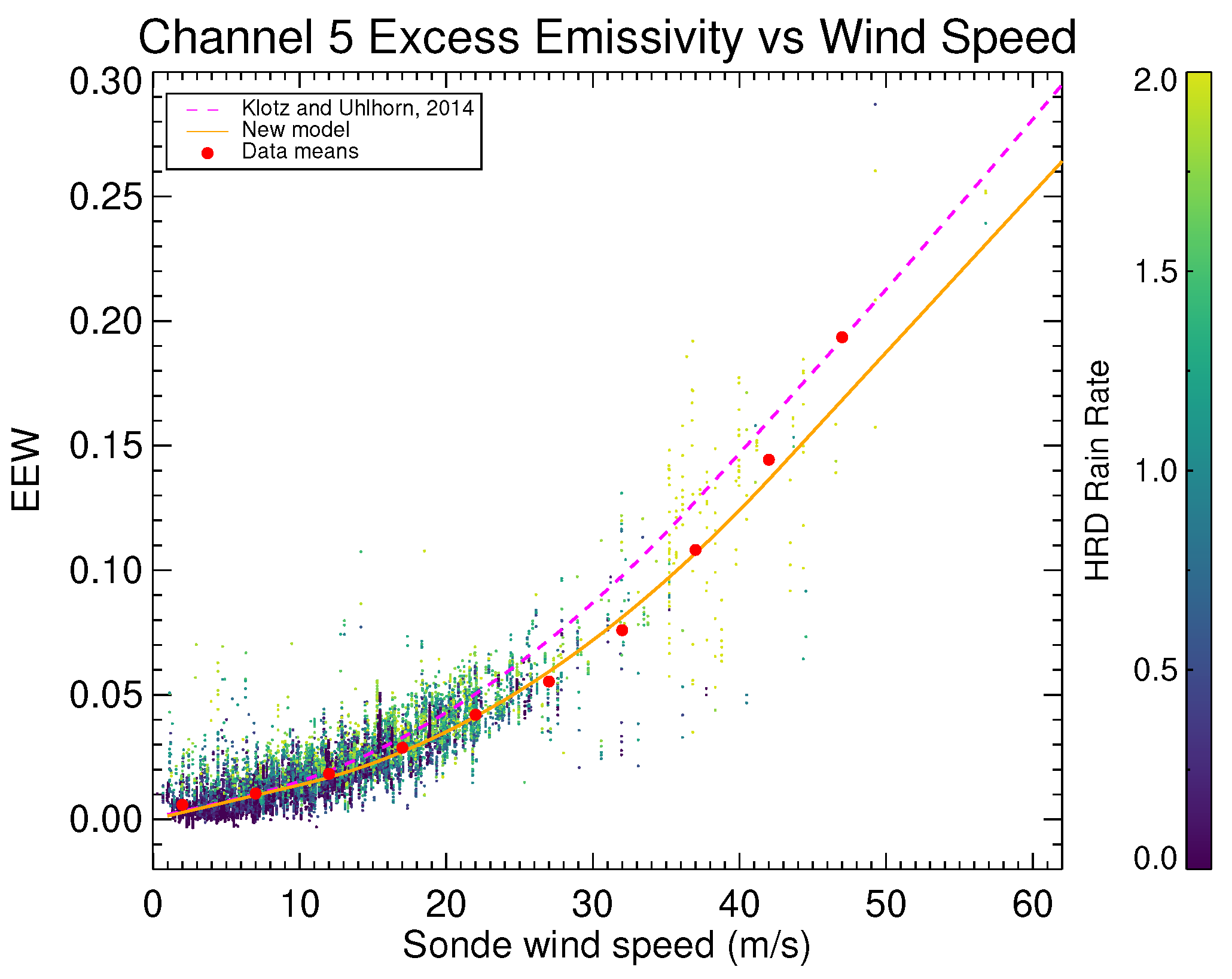
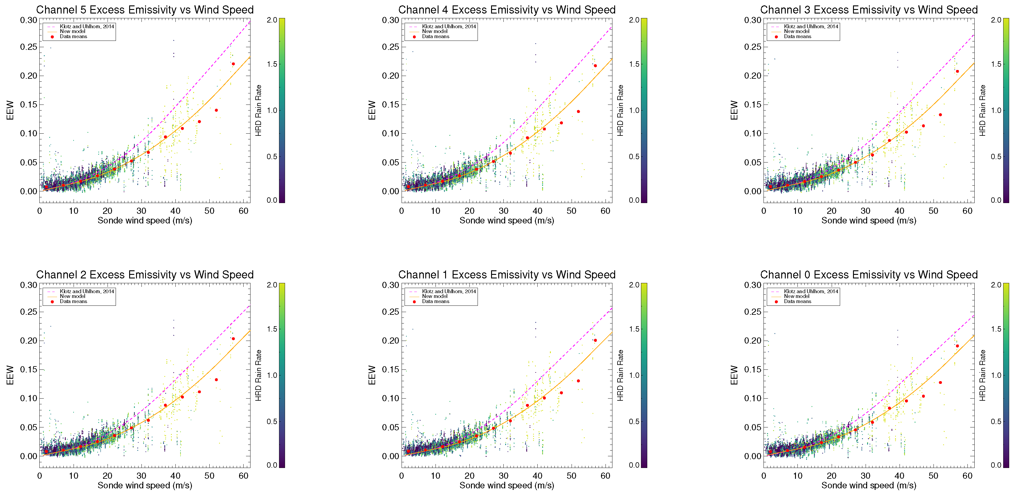
Figure 3 shows a scatter plot of SFMR channel 5 (highest frequency) EEW ( ε e ) as a function of dropsonde wind speed. Each point is colored according to its corresponding HRD rain rate. The solid line is the model developed from a straightforward application of the above methodology from the wind-speed-binned averages, and the dashed line is the current operational model from [8]. Since different dropsondes and slightly different filtering criteria are used, some small differences between the two can be expected. However, the new model shown is not sufficient to correct the observed wind-speed bias shown later in Figure 5.
The EEW estimates show a small trend with HRD-retrieved rain rate. EEW was estimated assuming no atmospheric effects and total ocean emissivity was assumed to only be affected by SST, salinity, and wind speed (e.g., not affected by rain) for the SFMR polarization, frequencies, and low incidence angles. This effect is therefore an unaccounted source of Tb that remains in the ε e estimate.
The most likely source is in the atmosphere: either the rain-free assumption does not apply, or the simple atmospheric models are not sufficiently detailed or capable of resolving minute Tb changes. Though it has long been understood that the low SFMR rain-rate retrievals ( < 10 mm h −1 [16] or, more recently, < 3 mm h −1 [8]) are nearing the low end of the sensitivity capabilities of the SFMR, the SFMR retrieval algorithm still reports them. This suggests that there is some information contained in the low rain rate retrievals, but it may not be rain rate. Regardless, if this excess Tb is not removed then it is included in the EEW estimate, inflating what is assumed to be emissivity solely from wind effects.
It could be argued that the observed trend is in reality a wind-speed dependence that was erroneously retrieved as rain rate. If that were the case, we would expect to see a trend with dropsonde wind speed introduced into the retrievals using the EEW model developed from this methodology. As we show later in Figure 5, there are no systematic biases introduced by this revision. In fact, the existing trend with wind speed is eliminated and errors present in rain are largely reduced.
The resulting EEW GMFs as functions of 10 m equivalent-neutral wind speed are shown as the solid lines passing through the filled circles (means) in Figure 4. To obtain the GMFs, EEW data is grouped into 5 m s −1-wide bins. The channel 5 means are fit to the coefficients in (5) using a Levenberg-Marquardt least-squares technique. Since there are few samples at high winds, the slope for channel 5 at 37 m s −1 (the previous a 0 from (5)) is retained from the current model. The 2014 SFMR GMFs are also shown for reference. At the lower end of the wind-speed range, the dropsonde error is close to the measured wind speed and SFMR is not capable of reliably sensing these wind speeds. As a result, we only use data above 10 m s −1 that have a significant number of points to generate the GMFs for (6) and the quadratic and high-wind linear portions of (5).
The wind-generated foam to which the SFMR is primarily sensitive does not exist below approximately 7 m s −1, the traditional transition point of the SFMR GMF from a linear function to a quadratic. In this manuscript the transition point was chosen such that the slope of the frequency-independent quadratic function matches a line that intercepts the origin. As a result, the slope of the linear portion was also allowed to vary. Referring to (5), this condition requires
a 2 + a 3 v l + a 4 v l 2 v l = a 3 + 2 a 4 v l a 2 v l = a 4 v l v l = a 2 a 4 10.5   m   s .
The a 1 coefficient is derived from v l , a 2 , a 3 , and a 4 to make a line from the origin meet the quadratic at v l . The values for a 0 a 9 are given in Table 3.
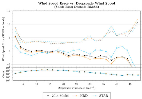
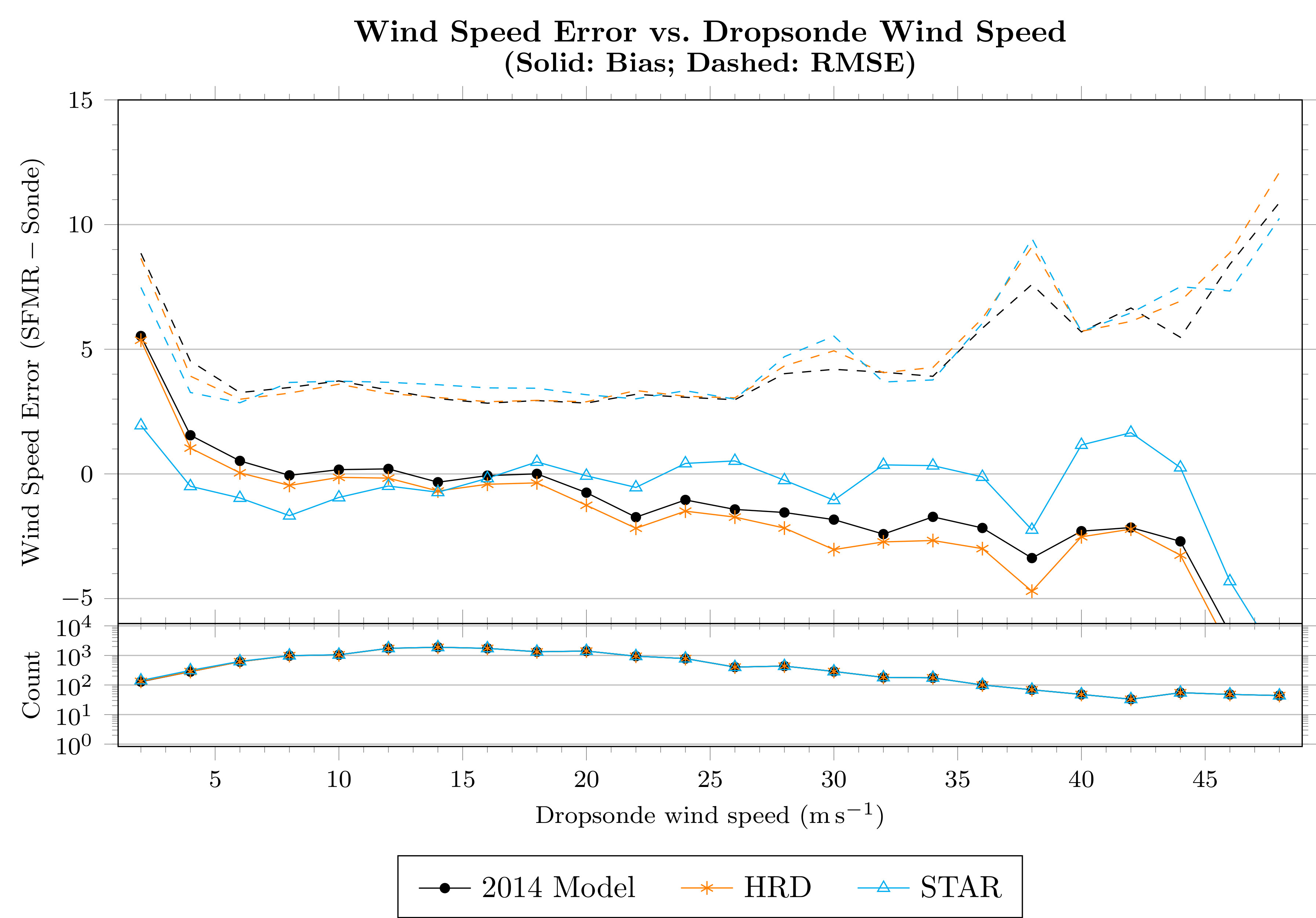
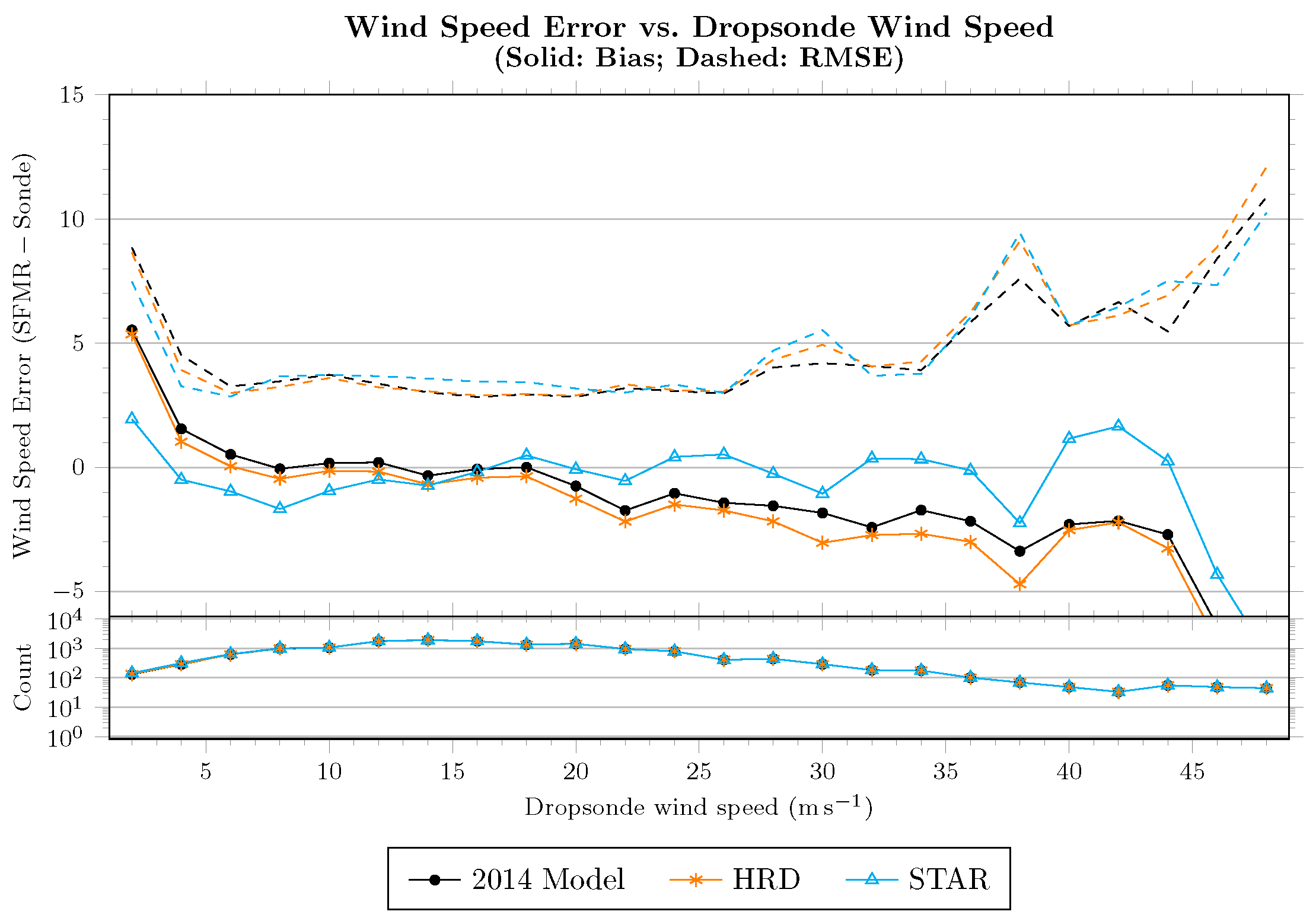
Figure 5 shows the wind-speed error as a function of dropsonde surface wind speed estimate, where error is defined as the SFMR retrieval less the dropsonde-estimated U 10 N . Retrievals using the model developed in this section (and, necessarily, the model from Section 2.4) are shown as empty blue triangles. Compared to both the retrievals performed by the authors with the 2014 models and the HRD retrievals (both of which have nearly the same characteristics), the mean error above 20 m s −1 is reduced while maintaining or improving the RMS error.
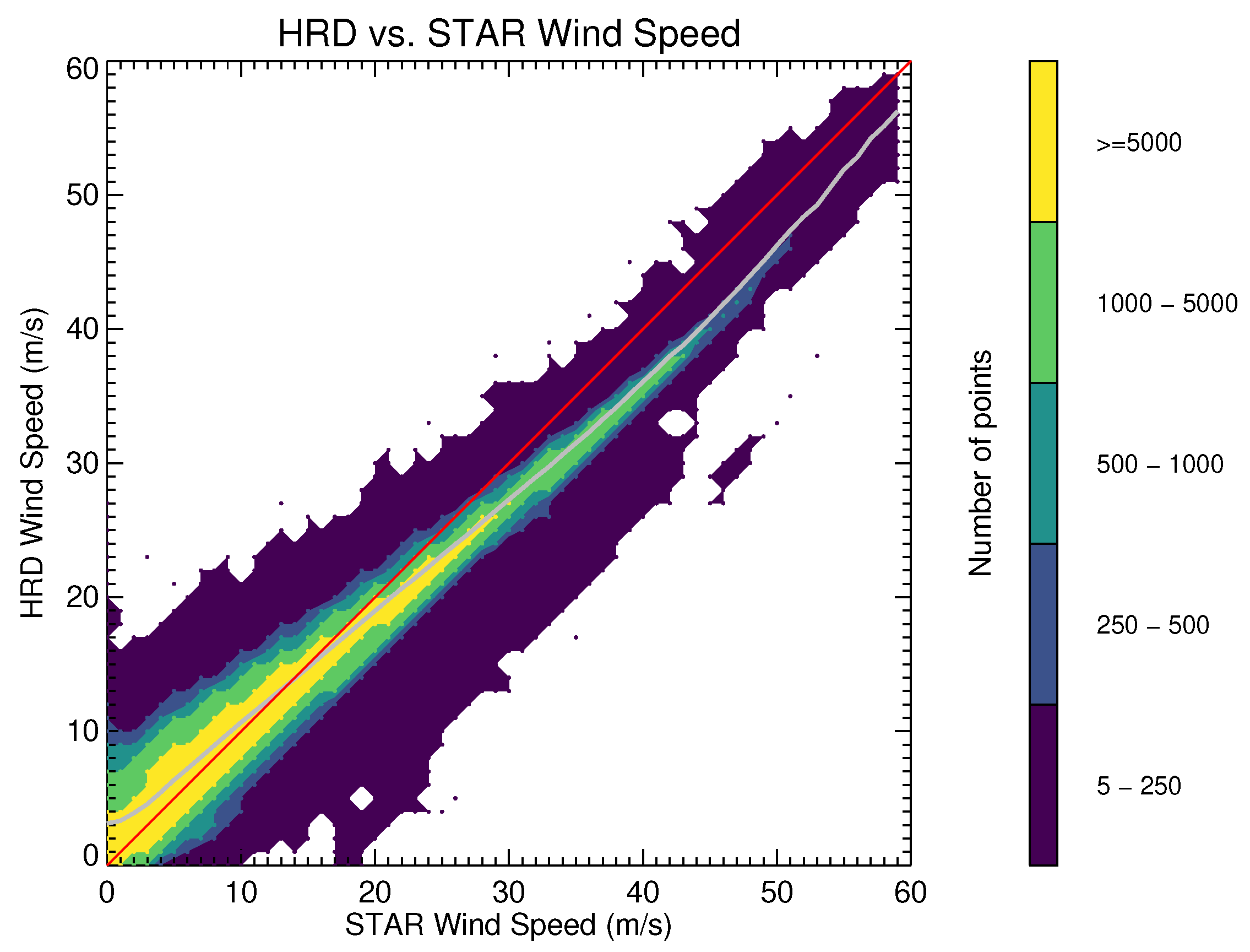
Figure 6 shows these HRD (left panel) and STAR (right panel) retrievals versus dropsonde surface wind speed as two-dimensional histograms. The number of points within each 1 by 1 m s −1 bin is averaged and shown as a color. Histograms for each axis are shown on the outside of the corresponding axis. The mean value of each ordinate is calculated from the points within each 1 m s −1 dropsonde bin and is shown as a solid orange line. Both show a general trend of the 2014 model (implemented by HRD here) to underestimate the dropsonde surface wind speed and that the STAR model better matches the dropsondes.

3.2. Rain

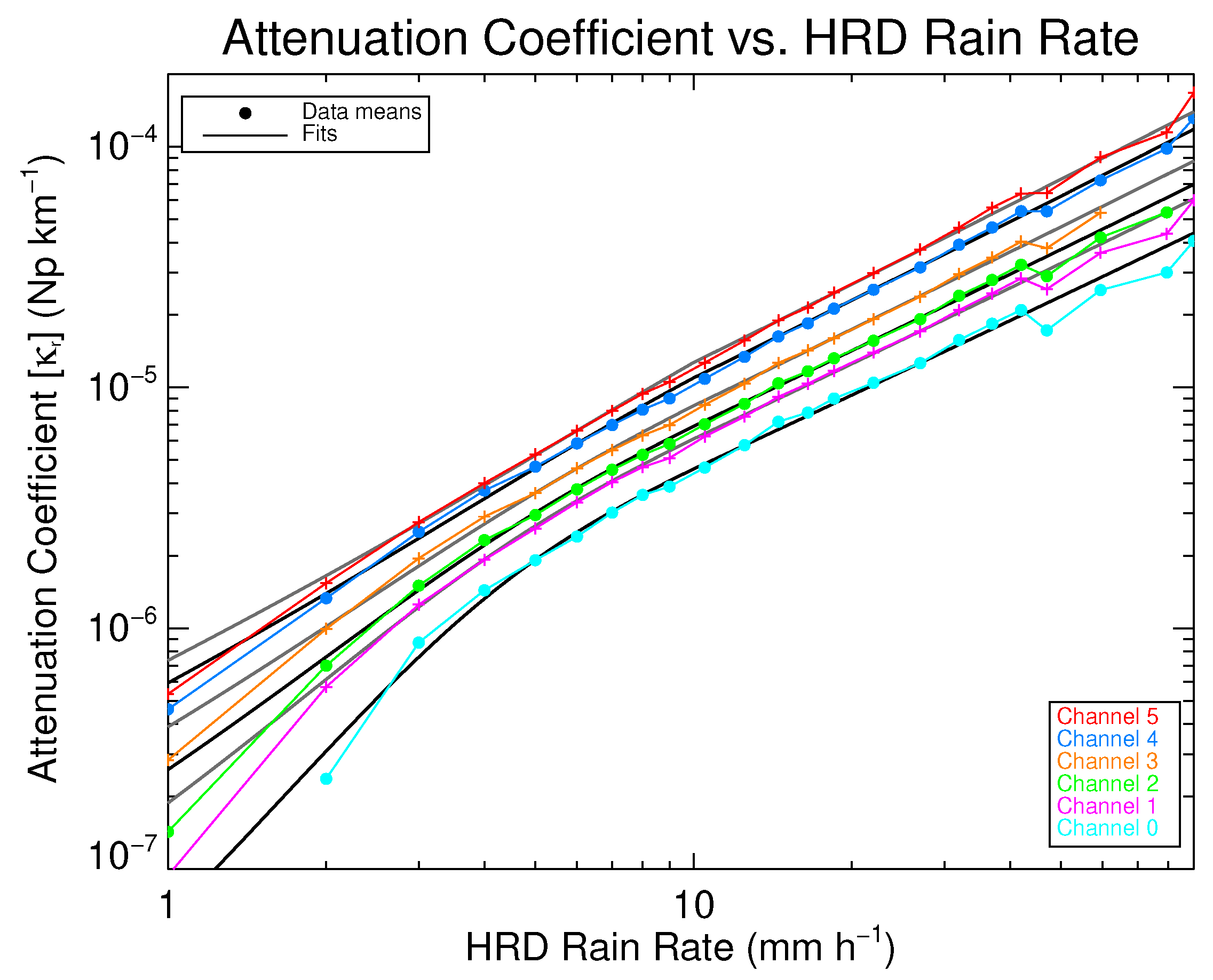
Figure 7 shows the estimated κ r from SFMR data as a function of the HRD rain-rate retrieval on a log-log plot. The solid lines are the fits to the data for each frequency (increasing in value with frequency) and the filled circles are the binned κ r averages. Immediately noticeable is the downward curve below 3 mm h −1, due to a lower sensitivity of the lower channels to rain at low rain rates and thus a higher variance of κ r . Though [8] provided a significant validation of higher rain-rate retrievals, the precision of rain-rate retrievals from SFMR at and below 3 mm h −1 should not be relied upon. The values of the absorption coefficients given in (8) are listed in Table 4.
Even though the precision may be lacking, a separate curve was fitted below 10 mm h −1 to avoid overestimating and to improve matching of STAR retrievals to those from HRD at low rain rates. The rain-absorption model used for rain rates below 10 mm h −1 in the STAR retrievals ( κ r ) is
P 0 = exp C 1 + C 2 f + C 3 f 2
P 1 = exp C 4 + C 5 f + C 6 f 2
κ r = κ r exp P 0 P 1 R ,
where κ r is from (8) and the coefficients are listed in Table 4 and Table 5.
One method of verifying that the newly retrieved rain rates are comparable to the HRD-retrieved rain rates is to use a two-dimensional histogram, shown in Figure 8. The data is colored by number of points in each 1 mm h −1 square, and most of the data is in the low rain rate bins. The new model generally produces the same results. Below 25 mm h −1, the STAR retrieval algorithm produces slightly lower rain rates than the HRD retrieval algorithm, and above 25 mm h −1 STAR produces higher rain rates. The largest discrepancies are at rain rates above 40 mm h −1, where there were few validation data used during development of the 2014 model (less than 10% of the data shown in g 8 of [8]).
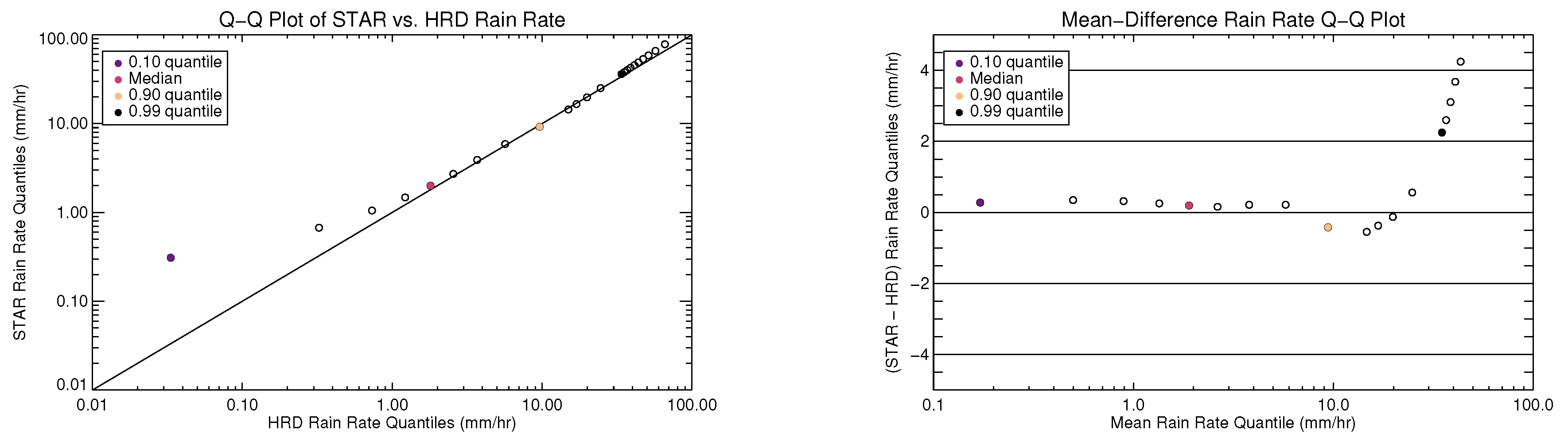
Two other methods of confirming the validity of the new model are shown in Figure 9: a quantile-quantile plot and a mean-difference plot of the quantiles. This is a way of evaluating the overall statistics rather than comparing retrievals from the same scene. All collocated scenes presented in Figure 8 were used to generate quantiles for each data set. The deciles are shown starting at 10%, as well as quantiles from 95 to 99% in 1% steps and 99 to 99.9% in 0.1% steps. The mean-difference plot shows the difference between the quantiles of the two datasets as a function of the means of each quantile pair. For example, the 10% quantile is plotted between 0.1 and 0.2 mm h −1 on the horizontal axis because the HRD value is approximately 0.03 and the value for the STAR retrievals is approximately 0.3.
These plots show that for the lowest 80% of the data ( < 9 mm h −1), the new retrievals are higher than the HRD retrievals by less than 0.5 mm h −1. This is the same behavior as when the model from [8] is implemented and compared against the HRD retrievals in the same way (e.g., the “2014 model” shown in Figure 5). For the lowest 98% of the data ( < 35 mm h −1), the new retrievals are different from the HRD retrievals by at most 2 mm h −1. Up to 40 mm h −1, the STAR retrievals are up to 4 mm h −1 (< 10%) higher than HRD. Though there are some differences in the output of the two retrieval algorithms, the differences are small ( < 2 mm h −1) in the regime where there are the most data. The rain rates output by the new model still represent the physical scene as well as SFMR can measure given its spatial and temporal footprint.
Figure 10 shows a comparison two-dimensional histogram between all collocated HRD and STAR wind-speed retrievals. A solid gray line shows the mean HRD wind speed for each wind speed retrieved by the new model. Above 15 m s −1 the STAR-model-retrieved wind speeds tend to exceed those retrieved by HRD. The maximum difference in the mean between the two is approximately 5 m s −1, which occurs at the highest wind speeds shown.
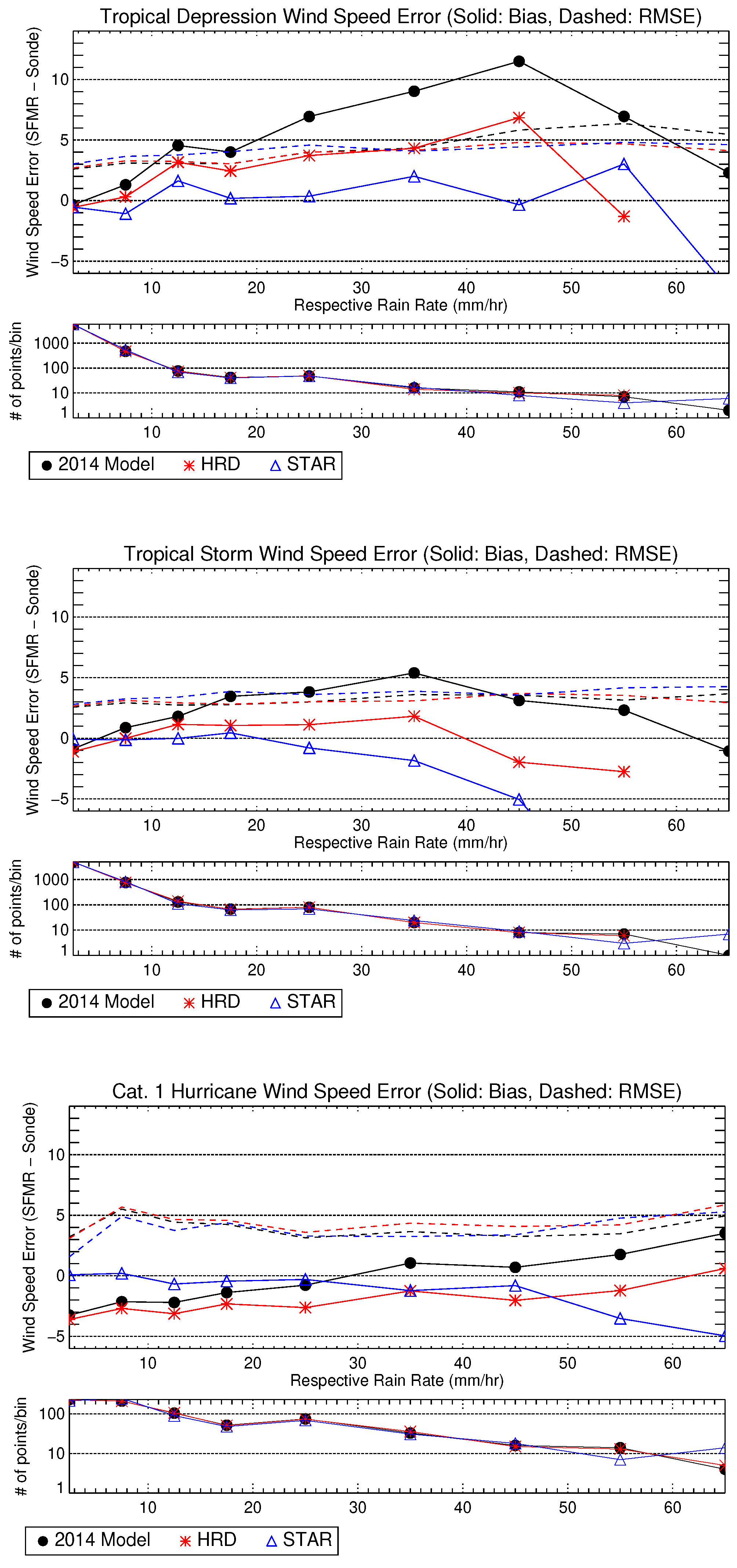
Figure 11 shows a comparison similar to the one at the end of [8] (i.e., Figure 14). There is a different selection of data used here, so some differences can be expected. The plots show wind-speed error (SFMR minus dropsonde U 10 N ) versus the rain rate retrieved by each of three algorithms: the “2014 model” described in [8], HRD, and STAR. The latter two have some additional filtering implemented beyond what is described in [8].
These figures suggest that rain above 10 mm h −1 do not necessarily indicate a high bias, sometimes called “rain contamination”, in the wind-speed retrievals. However, unlike [8], very little bias in the mean is found below approximately 45 mm h −1 in tropical storm conditions for either the HRD or STAR retrievals—though the retrievals performed by the authors just using the 2014 model more closely resemble their results. This suggests a rain-rate-dependent wind-speed correction is being applied to the HRD retrievals.
In “Category 1” hurricane conditions the HRD algorithm is generally biased low compared to dropsondes, but the STAR algorithm shows no wind-speed bias for rain rates up to at least 45 mm h −1. An important feature of the STAR retrievals is the lack of bias at rain rates below this threshold, which shows that rain does not necessarily contaminate SFMR wind-speed retrievals. Additionally, the RMS error for the STAR retrievals is lower than that of HRD up to 45 mm h −1, which is a reversal from the lower-wind observations. As a result of these data, we consider wind-speed retrievals questionable where the rain rate is at least 45 mm h −1.
In tropical storm conditions, there is no mean bias in the STAR algorithm below 45 mm h −1. Surprisingly, there is not as significant rain influence on wind-speed retrievals in low-wind (“Tropical Depression”) scenarios, though we would caution against using any SFMR wind-speed retrievals in this wind-speed regime. As a general rule, we suggest that the precision of wind-speed retrievals below 15 m s −1 should not be relied upon.
There is slightly more spread in the STAR retrievals (RMS errors) in the two lower-wind regimes compared to those from HRD. This is likely due to the differences in smoothing or filtering of the retrieval algorithms. The STAR filtering criteria were chosen to retain high-wind gradients while reducing geophysical and system noise and thus can be expected to exhibit more scatter at all wind speeds.
Table 6, Table 7 and Table 8 show means, standard deviations, and number of samples of SFMR errors (versus dropsondes) within selected wind-speed and rain-rate bins. As shown on the above plots, the STAR mean errors are generally closer to 0 than those from HRD except in the highest rain-rate group ( 30 mm h −1). The increased spread of the STAR retrievals is evident in that the standard deviations are slightly higher in all regimes.

4. Discussion

The results above show improvement of SFMR wind-speed retrievals compared to dropwindsondes in tropical storm to hurricane wind conditions. Compared to the most recent revision of the operational SFMR GMFs [8], the wind-speed differences between retrievals and dropsondes were reduced by as much as 10% at wind speeds in excess of 45 m s −1. Additionally, the GMFs presented in this manuscript improve the biases experienced in rain—also referred to as “rain contamination.” These changes result in generally higher wind-speed retrievals in high-wind conditions and lower retrievals at wind speeds less than 15 m s −1. However, due to the low sensitivity of SFMR to wind speed at low surface wind speeds relative to other small-scale roughness factors the precision of these low-wind retrievals is highly questionable.
Improving wind-speed retrievals required a change to the C-band liquid water absorption coefficient model used to retrieve rain rate, due to the simultaneous nature of the retrieval algorithm. The rain rates generally remained the same, as far as they could be reasonably validated. Above 25 mm h −1, the rain-rate retrievals from the GMF presented here are higher than those from the current operational model by up to 10 mm h −1. However, this is the regime in which there are the fewest data for validation; certainly, this is an area of possible improvement for a collocated rain-sensing instrument, such as a radar or precipitation sensor collocated with SFMR on an aircraft. Due to the weak response of precipitation at C-band at rain rates lower than 3 mm h −1, low-rain retrievals cannot be relied upon to be accurate.
One limitation of the instrument is the frequency stepping operation and internal brightness temperature smoothing. While they have their advantages, they smear or overlook sharp wind gradients and small rain bands. This ultimately limits the resolution of SFMR. A microwave radiometer that samples C-band frequencies simultaneously (e.g., [25]) could help to identify some geophysical limitations of the historical SFMR archive.
Roughness effects due to the splash of precipitation and sea state have not been accounted for in the SFMR RTM. At the wind speeds typically measured by SFMR and used by researchers and forecasters ( > 20 m s −1), the roughening effect of precipitation has a significantly weaker contribution than the wind-generated foam on the brightness temperature observed by the instrument. In this manuscript we go one step towards including these modifications to surface emissivity in the RTM by adding the Ω term to (4). However, there likely remain residual roughness effects due to rain and sea state and they should be investigated more quantitatively. As a result, the retrieval errors dependent on these factors (e.g., storm quadrant [10]) remain unaddressed.
Atmospheric and smooth-surface emissivity models were brought more in line with the current literature, but they are still only models. In particular, the downwelling radiation or atmospheric profiles from above the aircraft could be measured to study possible improvements to surface wind-speed and rain-rate estimation.

5. Conclusions

Since the deployment of the Stepped Frequency Microwave Radiometer (SFMR) as an instrument used in operational forecasting and warning, hurricane reconnaissance and research aircraft have been providing near real-time observations of the 10 m equivalent-neutral ocean-surface wind speed in and around tropical storms and cyclones. Hurricane specialists use these data to assist in determining wind radii and maximum sustained winds—critical parameters for determining and issuing watches and warnings. These observations are also being used for post-storm analysis, model validation, and even ground truth for aircraft- and satellite-based wind sensors; the international ocean winds community will increasingly rely on SFMR for high-wind calibration and validation. It is imperative that any errors in these observations be understood and reduced as much as possible. Uncertainty in the SFMR brightness temperature measurements can have significant implications on the near real-time use of SFMR data for TC forecasting, post-storm analysis, and climatological studies.
SFMR retrievals from the most recent SFMR geophysical model function (GMF) show a 10% low wind speed bias when compared with global positioning system dropsondes up to 45 m s −1. Correcting this primarily required correction to the excess emissivity due to wind (EEW) model. In the process we updated the atmospheric and smooth-surface ocean emissivitymodels at C-band.Anewfit of the EEWand rain-absorption coefficients used in the SFMR retrieval algorithm removed the wind-speed bias observed with the dropsondes. So-called “rain contamination” of the retrieved wind speed below 45 mm h −1, described in [8], was also removed. There remains a low precision for low wind speed ( < 15 m s −1) and low rain rate ( < 10 mm h −1) retrievals, but these are due to hardware limitations of the instrument and geophysical effects that must be better understood. Though there are few reference wind speeds above 45 m s −1 available for validation, the new SFMR retrievals are consistent with those that do exist.
Implementing these new models in both the operational and post-processing SFMR retrieval algorithms will result in improved and consistent SFMR wind and rain-rate measurements to support tropical cyclone forecasting and subsequent climate studies. To support operational use of unbiased SFMR wind and rain-rate measurements, we recommend that these newly developed models be implemented in the operational SFMR retrieval algorithm. We also recommend that the calibration procedure remain unchanged, as consistency throughout the data record is critical. These models were developed to not require changes to the ocean calibration procedures.
The NOAA/NESDIS Ocean Surface Winds Team makes available a database of all files produced by the methods described in this manuscript. The data files have a consistent set of variables with metadata complying with the CF-1.6 standards. Supplementary data (e.g., sea-surface temperature (SST) and salinity) are from a consistent source for the entire time span of the data and are documented in each file. A quality flag is provided which indicates invalid and questionable retrievals (e.g., when rain rates above 45 mm h −1 are retrieved). Data are available at https://manati.star.nesdis.noaa.gov/SFMR.

Author Contributions

Conceptualization, J.W.S., S.O.A., Z.J., P.S.C. and J.C.; Data curation, J.W.S.; Formal analysis, J.W.S. and S.O.A.; Funding acquisition, Z.J. and P.S.C.; Investigation, J.W.S., S.O.A., Z.J. and J.C.; Methodology, J.W.S., S.O.A., Z.J. and P.S.C.; Project administration, Z.J. and P.S.C.; Resources, P.S.C.; Software, J.W.S., S.O.A. and J.C.; Supervision, Z.J., P.S.C. and J.C.; Validation, J.W.S. and S.O.A.; Visualization, J.W.S. and S.O.A.; Writing—original draft, J.W.S. and J.C.; Writing—review & editing, J.W.S., S.O.A., Z.J., P.S.C. and J.C.

Funding

This research was funded by the National Oceanic and Atmospheric Administration contract number ST-1330-17-CQ-0050.

Acknowledgments

The authors would like to thank the NOAA/NESDIS Ocean Remote Sensing Program for its support of their flight experiment program; the NOAA Aircraft Operations Center and the U.S. Air Force Reserve Command for their assistance with providing and collecting the data on which this paper is based; and S. Frasier of the University of Massachusetts Amherst for software improvements in the SFMR RTM code.

Conflicts of Interest

The authors declare no conflict of interest. The funders had no role in the design of the study; in the collection, analyses, or interpretation of data; in the writing of the manuscript, or in the decision to publish the results.

Abbreviations

The following abbreviations are used in this manuscript:
AFRCU.S. Air Force Reserve Command
EEWexcess emissivity due to wind
EIAEarth-incidence angle
GMFgeophysical model function
HRDNOAA Hurricane Research Division
NESDISNational Environmental Satellite, Data, and Information Service
NHCNational Hurricane Center
NOAANational Oceanic and Atmospheric Administration
RFIradio frequency interference
RSSRemote Sensing Systems
RTMradiative transfer model
SFMRStepped Frequency Microwave Radiometer
SSTsea-surface temperature
STARCenter for Satellite Applications and Research
Tbbrightness temperature

Appendix A. Rain Transmissivity Estimation Derivation

The SFMR radiative transfer model (RTM) gives the total brightness temperature observed as
T b = τ r , a τ a , a T b , o c e a n + ( 1 ε ) T b , s k y + T b , u p ,
where
T b , o c e a n = ε T S
T b , s k y = T b , d o w n + τ r , τ a , T b , c o s + T b , s c a t
T b , d o w n = ( 1 τ r , ) T r , + τ r , T a , ( 1 τ a , )
T b , u p = 1 τ r , a τ a , a T a , a ,
and T b , c o s = 2.73   K . We will solve for τ r , a , the transmissivity of the atmosphere below the aircraft. (A1) becomes
T b = τ r , a τ a , a ε T S + ( 1 ε ) T b , s k y T a , a + T a , a = τ r , a τ a , a ε T S T a , a + τ r , a τ a , a ( 1 ε ) T b , s k y + T a , a ,
which, when combining all terms on one side of the equation, becomes:
T b T a , a + τ a , a τ r , a T a , a ε T S τ a , a τ r , a T b , s k y ( 1 ε ) = 0
τ r , a τ r , = exp ( κ h sec θ ) exp ( κ H r sec θ ) = exp ( κ sec θ ( h + H r ) ) = exp ( κ h sec θ ( 1 + H r h ) ) = exp ( κ h sec θ ) ( 1 + H r h ) = τ r , a ( 1 + H r h )
τ r , a T b , s k y is expanded to
τ r , a T b , s k y = τ r , a ( 1 τ r , ) T r , + τ r , T a , ( 1 τ a , ) + τ r , τ a , T b , c o s + T b , s c a t = τ r , a ( 1 τ r , ) T r , + τ r , a τ r , T a , ( 1 τ a , ) + τ r , a τ r , τ a , T b , c o s + τ r , a T b , s c a t = τ r , a T r , + T b , s c a t τ r , a τ r , T r , + τ r , a τ r , T a , ( 1 τ a , ) + τ r , a τ r , τ a , T b , c o s = τ r , a T r , + T b , s c a t τ r , a ( 1 + H r h ) T r , + τ r , a ( 1 + H r h ) T a , ( 1 τ a , ) + τ r , a ( 1 + H r h ) τ a , T b , c o s = τ r , a T r , + T b , s c a t τ r , a ( 1 + H r h ) T r , T a , ( 1 τ a , ) τ a , T b , c o s .
So (A7) becomes
T b T a , a + τ r , a τ a , a T a , a ε T S ( 1 ε ) T r , + T b , s c a t + τ r , a ( 1 + H r h ) τ a , a 1 ε T r , T a , ( 1 τ a , ) τ a , T b , c o s = 0 .
Finally, we arrange the equation to calculate τ r , a
c 0 τ r , a ( 1 + H r h ) + c 1 τ r , a + c 2 = 0 ,
where
c 0 = τ a , a ( 1 ε ) T r , T a , ( 1 τ a , ) τ a , T b , c o s ,
c 1 = τ a , a T a , a ε T S ( 1 ε ) T r , + T b , s c a t ,
c 2 = T b T a , a .
Please note that though this result is similar to that presented in [8], it is not the same—even when neglecting T b , s c a t . Using their formulas resulted in unrealistically low rain transmissivities ( τ r ) for C-band.

Appendix B. Brightness Temperature Bias Correction

As stated in Section 2.3.2, the tuning error of the SFMR is a calibration error and is defined as the mean difference between the measured Tb and the SFMR GMF-predicted value. This typically appears when there is an error in deriving the calibration coefficients for a given instrument, either during the calibration procedure or post-processing. To reduce the effects of the tuning error on wind-speed and rain-rate retrievals, a bias-correction algorithm is run on the brightness temperatures before retrieval.
For each flight, retrievals are performed as usual. For each channel with wind speeds between 15 and 30 m s −1 and at most 3 mm h −1 of rain collected below 5 km altitude over the ocean, the following bias estimation routine is run. The mean difference for each retrieval between measured and modeled Tb is calculated and points more than two standard deviations away from the mean are eliminated. From this a preliminary estimate of the per-channel tuning error is obtained. This vector of biases is adjusted to have a mean of zero and any channel with a bias of more than 2 is omitted from bias estimation and retrieval. These bias corrections are then applied to the measured brightness temperatures. The final Tb used for retrieval is
T b , f i n a l = T b T b , b i a s .
Figure A1 shows histograms of measured Tb less modeled Tb for a flight with observable tuning errors. The flight was through Hurricane Earl on 2 September 2010 by an AFRC aircraft (so no radio frequency interference (RFI) from other scientific equipment on the aircraft is expected). This was the first storm flight of the 2010 hurricane season for this SFMR unit, and it does not seem to have flown often. However, the flight on 17 September 2010 by the same unit exhibits the same characteristics, suggesting that this is not unique to the local environment (e.g., RFI from nearby transmitters) or the storm conditions. The histograms labeled “HRD” use Tbs from the NOAA Hurricane Research Division (HRD) SFMR data files and subtract the modeled Tbs computed from [8]. Those labeled STAR use the retrievals and models presented in this manuscript after bias correction—the models make only a small difference, so the bias-correction procedure is the cause of the difference in mean error. Channel 3 has the largest bias of close to 1 K , but the other channels still have a distribution with a longer tail on the higher side. For all channels, the bias-correction procedure removes the mean biases in each channel and improves the accuracy of retrievals when compared to the GMF.
Figure A1. Tb tuning error by channel for the 20100902US017 AFRC flight. Numbers in the upper right corner correspond to number of data points contained in each histogram. There are differences due to different flagging and filtering criteria for each source (HRD or STAR) and for each channel.
Remotesensing 11 00214 g0a1
This is implemented in the STAR post-processing algorithm, so it is not applied in real-time. However, if this analysis is used to detect tuning biases early in the hurricane season it may be able to be corrected for in subsequent flights.

References

  1. Uhlhorn, E.W.; Black, P.G. Verification of Remotely Sensed Sea Surface Winds in Hurricanes. J. Atmos. Ocean. Technol. 2003, 20, 99. [Google Scholar] [CrossRef]
  2. Jones, W.L.; Black, P.G.; Delnore, V.E.; Swift, C.T. Airborne Microwave Remote-Sensing Measurements of Hurricane Allen. Science 1981, 214, 274–280. [Google Scholar] [CrossRef] [PubMed]
  3. Rogers, R.; Aberson, S.; Black, M.; Black, P.; Cione, J.; Dodge, P.; Gamache, J.; Kaplan, J.; Powell, M.; Dunion, J.; et al. The Intensity Forecasting Experiment: A NOAA Multiyear Field Program for Improving Tropical Cyclone Intensity Forecasts. Bull. Am. Meteorol. Soc. 2006, 87, 1523–1537. [Google Scholar] [CrossRef]
  4. Rappaport, E.N.; Franklin, J.L.; Avila, L.A.; Baig, S.R.; Beven, J.L.; Blake, E.S.; Burr, C.A.; Jiing, J.G.; Juckins, C.A.; Knabb, R.D.; et al. Advances and Challenges at the National Hurricane Center. Weather Forecast. 2009, 24, 395–419. [Google Scholar] [CrossRef] [Green Version]
  5. Beven, J.L.; Avila, L.A.; Blake, E.S.; Brown, D.P.; Franklin, J.L.; Knabb, R.D.; Pasch, R.J.; Rhome, J.R.; Stewart, S.R. Atlantic Hurricane Season of 2005. Mon. Weather Rev. 2008, 136, 1109–1173. [Google Scholar] [CrossRef] [Green Version]
  6. Stepped Frequency Microwave Radiometer (SFMR)—ProSensing. Available online: http://www.webcitation.org/query?url=http%3A%2F%2Fwww.prosensing.com%2Fcrb-product%2Fsfmr%2F&date=2018-11-28 (accessed on 28 November 2018).
  7. Ulaby, F.T.; Moore, R.K.; Fung, A.K. Microwave Remote Sensing: Fundamentals and Radiometry; Addison-Wesley Pub. Co. Advanced Book Program/World Science Division: Reading, MA, USA, 1981; Volume 1. [Google Scholar]
  8. Klotz, B.W.; Uhlhorn, E.W. Improved Stepped Frequency Microwave Radiometer Tropical Cyclone Surface Winds in Heavy Precipitation. J. Atmos. Ocean. Technol. 2014, 31, 2392–2408. [Google Scholar] [CrossRef]
  9. Meissner, T.; Wentz, F.J. The Emissivity of the Ocean Surface Between 6 and 90 GHz Over a Large Range of Wind Speeds and Earth Incidence Angles. IEEE Trans. Geosci. Remote Sens. 2012, 50, 3004–3026. [Google Scholar] [CrossRef]
  10. Powell, M.D.; Uhlhorn, E.W.; Kepert, J.D. Estimating Maximum Surface Winds from Hurricane Reconnaissance Measurements. Weather Forecast. 2009, 24, 868–883. [Google Scholar] [CrossRef]
  11. Hollinger, J.P. Passive Microwave Measurements of Sea Surface Roughness. IEEE Trans. Geosci. Electron. 1971, 9, 165–169. [Google Scholar] [CrossRef]
  12. Nordberg, W.; Conaway, J.; Ross, D.B.; Wilheit, T. Measurements of Microwave Emission from a Foam-Covered, Wind-Driven Sea. J. Atmos. Sci. 1971, 28, 429–435. [Google Scholar] [CrossRef] [Green Version]
  13. Uhlhorn, E.W.; Black, P.G.; Franklin, J.L.; Goodberlet, M.; Carswell, J.; Goldstein, A.S. Hurricane Surface Wind Measurements from an Operational Stepped Frequency Microwave Radiometer. Mon. Weather Rev. 2007, 135, 3070–3085. [Google Scholar] [CrossRef]
  14. Wentz, F.J.; Mattox, L.A.; Peteherych, S. New Algorithms for Microwave Measurements of Ocean Winds: Applications to Seasat and the Special Sensor Microwave Imager. J. Geophys. Res. 1986, 91, 2289. [Google Scholar] [CrossRef]
  15. Fernandez, D.E.; Kerr, E.M.; Castells, A.; Carswell, J.R.; Shaffer, S.J.; Chang, P.S.; Black, P.G.; Marks, F.D. IWRAP: The Imaging Wind and Rain Airborne Profiler for Remote Sensing of the Ocean and the Atmospheric Boundary Layer within Tropical Cyclones. IEEE Trans. Geosci. Remote Sens. 2005, 43, 1775–1787. [Google Scholar] [CrossRef]
  16. Jiang, H.; Black, P.G.; Zipser, E.J.; Marks, F.D., Jr.; Uhlhorn, E.W. Validation of Rain-Rate Estimation in Hurricanes from the Stepped Frequency Microwave Radiometer: Algorithm Correction and Error Analysis. J. Atmos. Sci. 2006, 63, 252–267. [Google Scholar] [CrossRef]
  17. Hock, T.F.; Franklin, J.L. The NCAR GPS Dropwindsonde. Bull. Am. Meteorol. Soc. 1999, 80, 407–420. [Google Scholar] [CrossRef] [Green Version]
  18. Franklin, J.L.; Black, M.L.; Valde, K. GPS Dropwindsonde Wind Profiles in Hurricanes and Their Operational Implications. Weather Forecast. 2003, 18, 32–44. [Google Scholar] [CrossRef]
  19. Sapp, J.W.; Alsweiss, S.O.; Jelenak, Z.; Chang, P.S.; Frasier, S.J.; Carswell, J. Airborne Co-Polarization and Cross-Polarization Observations of the Ocean-Surface NRCS at C-Band. IEEE Trans. Geosci. Remote Sens. 2016, 54, 5975–5992. [Google Scholar] [CrossRef]
  20. Liu, W.T.; Tang, W. Equivalent Neutral Wind; JPL Publication 96-17; National Aeronautics and Space Administration, Jet Propulsion Laboratory, California Institute of Technology: Pasadena, CA, USA, 1996.
  21. Current Hurricane Data Sets. Available online: http://www.aoml.noaa.gov/hrd/data_sub/hurr.html (accessed on 18 January 2019).
  22. Goodberlet, M.; Mead, J. Two-Load Radiometer Precision and Accuracy. IEEE Trans. Geosci. Remote Sens. 2006, 44, 58–67. [Google Scholar] [CrossRef]
  23. Klein, L.A.; Swift, C.T. An Improved Model for the Dielectric Constant of Sea Water at Microwave Frequencies. IEEE J. Ocean. Eng. 1977, 2, 104–111. [Google Scholar] [CrossRef]
  24. Wentz, F.J.; Meissner, T. Atmospheric Absorption Model for Dry Air and Water Vapor at Microwave Frequencies below 100 GHz Derived from Spaceborne Radiometer Observations: Atmospheric Absorption Model. Radio Sci. 2016, 51, 381–391. [Google Scholar] [CrossRef]
  25. Knapp, E.J.; Carswell, J.R.; Swift, C.T. A Dual Polarization Multi-Frequency Microwave Radiometer. In Proceedings of the IEEE 2000 International Geoscience and Remote Sensing Symposium, Honolulu, HI, USA, 24–28 July 2000; Volume 7, pp. 3160–3162. [Google Scholar] [CrossRef]
Figure 1. Block diagram for the Monte-Carlo simulation used to estimate the sensitivity to the calibration/tuning error.
Remotesensing 11 00214 g001
Figure 2. Rain-rate bias error versus the 10 m ocean-surface wind-speed bias error with a true rain rate of 10 mm h −1 and the different wind conditions labeled in each panel. Each SFMR channel was allowed a tuning error of −1.0, −0.5, 0.0, 0.5 or 1.0 K , resulting in 15,625 different cases for each wind condition.
Remotesensing 11 00214 g002
Figure 3. Uncorrected excess emissivity due to wind as a function of dropsonde wind speed. Colors on the small points indicate the associated HRD rain rate. Solid circles are means in 5° bins starting at 2 m s −1. The dashed line is the operational GMF [8] and the solid line is the GMF derived from the data points above 10 m s −1.
Remotesensing 11 00214 g003
Figure 4. Corrected excess emissivity due to wind as a function of dropsonde wind speed. Also shown are the means in 5 m s −1 bins as filled circles and a fit to the means according to (5) as a solid line. The dashed line is the 2014 EEW model from [8]. The fit was only performed to means with a sufficient number of samples above 10 m s −1.
Remotesensing 11 00214 g004
Figure 5. Wind-speed error (SFMR - dropsonde) as a function of dropsonde surface wind-speed ( U 10 N ) estimate for retrievals using the model from Klotz and Uhlhorn [8] (“2014 model”), the HRD dataset, and the STAR algorithm. Please note that the STAR algorithm includes the models from Section 2.3 and Section 2.4. Solid lines and symbols indicate means and dashed lines indicate the RMS error on the upper panel. The lower panel shows a histogram of the collocated data. Only collocations where all sources are available are included.
Remotesensing 11 00214 g005
Figure 6. SFMR wind-speed error as a function of dropsonde surface wind speed ( U 10 N ) estimate for both HRD and STAR retrievals. Points are colored by the number of points in each two-dimensional bin. One-dimensional histograms are shown for each 1 m s −1 bin on the left for retrievals and bottom for dropsondes. A solid orange line indicates the mean of the vertical axis for each horizontal bin.
Remotesensing 11 00214 g006
Figure 7. SFMR-estimated κ r (using the new EEW model) as a function of collocated HRD rain rate.
Remotesensing 11 00214 g007
Figure 8. Two-dimensional histogram of the HRD rain rate vs. rain rate produced by the model developed in this manuscript from all collocated data available. The solid gray line shows the mean in each 1 mm h −1 bin on the horizontal axis.
Remotesensing 11 00214 g008
Figure 9. Rain-rate distribution comparisons between the STAR retrievals and the HRD retrievals from all collocated data available. The left panel shows a log-log quantile-quantile plot comparing the STAR and the HRD retrievals. The right panel shows the mean-difference plot of the same two datasets with only the horizontal axis shown in a logarithmic scale. The lowest quantile shown is the 10% quantile with the remainder increasing in 10% steps up to 90%, then in 1% steps up to 99%, then in 0.1% steps up to 99.9%.
Remotesensing 11 00214 g009
Figure 10. Two-dimensional histogram of the HRD wind speed vs. wind speed produced by the model developed in this manuscript from all collocated data available. The solid gray line shows the mean in each 1 m s −1 bin on the horizontal axis. The solid red line is the y = x line.
Remotesensing 11 00214 g010
Figure 11. Wind-speed error (SFMR - dropsonde) as a function of rain rate for selected wind-speed regimes. From top to bottom the rows show results from tropical depression conditions (9 to 17 m s −1), tropical storm conditions (14 to 22 m s −1), and hurricane conditions (29 to 37 m s −1). The plots show wind-speed error means (solid lines) and RMS errors (dashed lines) versus the retrieved rain rate for the authors’ implementation of the 2014 model [8], the HRD retrievals, and the STAR algorithm. Differences between the “2014 model” and the HRD retrievals suggest a rain-rate-dependent wind-speed correction is being applied to the HRD retrievals.
Remotesensing 11 00214 g011
Table 1. Coefficients for the New Atmospheric Transmissivity Models.
ParameterValue
p 0 2.5623 × 10 4
p 1 5.9305 × 10 5
p 2 6.9957 × 10 5
p 3 1.1919 × 10 4
p 4 3.1739 × 10 3
p 5 1.8665 × 10 2
Table 2. Filtering criteria for SFMR and dropsonde collocations in tropical cyclones.
ParameterCriteria
Time between SFMR and sonde splash 10 min
Distance from SFMR to sonde 15
Absolute aircraft roll angle during 10 s average<3
Absolute aircraft pitch angle during 10 s average<3
Minimum aircraft altitude 1
sea-surface temperature 22   C
Dropsonde fall time through 150 m layer > 5 s
Table 3. New Coefficients of the Model for Excess Emissivity Due to Wind.
ParameterValue
a 0 54.4731
a 1 1.3925 × 10 3
a 2 6.2744 × 10 3
a 3 1.9859 × 10 4
a 4 5.6794 × 10 5
a 5 1.6225 × 10 1
a 6 6.3861 × 10 3
a 7 3.1048 × 10 4
a 8 7.2806 × 10 5
a 9 1.5913 × 10 6
Table 4. New Coefficients of the Model for Rain Absorption Above 10 mm h−1.
gcdb
1.5037 × 10 8 2.2005 6.0000 × 10 2 7.7707 × 10 1
Table 5. Coefficients of the Model for Rain Absorption Below 10 mm h−1.
C 1 C 2 C 3 C 4 C 5 C 6
10.5900−2.76651.7001 × 10−1−6.4871 × 10−23.5235 × 10−1−4.4598 × 10−2
Table 6. Wind-Speed Retrieval Error Means for the HRD and STAR Algorithms.
Rain Rate (mm h 1 )0 to 55 to 1010 to 20
Wind Speed m s 1 HRDSTARHRDSTARHRDSTAR
15 20 7.83 × 10 1 1.94 × 10 1 4.72 × 10 1 1.57 × 10 1 1.28 1.82 × 10 1
20 25 −1.99 2.84 × 10 2 −1.25 3.53 × 10 1 2.47 × 10 1 1.03
25 30 −2.40 5.26 × 10 1 −1.79 1.53 × 10 1 −1.62 3.66 × 10 3
30 40 −3.87 4.09 × 10 3 −3.67 4.70 × 10 3 −1.481.70
40 −8.75−8.54−5.75−1.79−5.09−1.27
Rain Rate (mm h 1 )20 to 30≥30
Wind Speed m s 1 HRDSTARHRDSTAR
15 20 1.82 3.39 × 10 1 −1.79−6.90
20 25 7.00 × 10 1 1.79 × 10 1 1.67−1.03
25 30 −2.18−1.35−1.93−3.70
30 40 −1.92 7.05 × 10 1 −2.74−2.17
40 −5.76−1.09−4.31−3.71
Table 7. Wind-Speed Retrieval Error Standard Deviations for the HRD and STAR Algorithms.
Rain Rate (mm h 1 )0 to 55 to 1010 to 2020 to 30≥30
Wind Speed m s 1 HRDSTARHRDSTARHRDSTARHRDSTARHRDSTAR
15 20 2.703.172.924.053.183.643.774.854.345.64
20 25 2.522.992.362.932.693.822.902.943.684.67
25 30 3.063.613.314.063.504.454.885.546.119.19
30 40 3.714.264.074.664.274.324.195.066.196.85
≥408.4810.215.666.686.076.057.418.146.887.43
Table 8. Wind-Speed Retrieval Error Counts for the HRD and STAR Algorithms.
Rain Rate (mm h 1 )0 to 55 to 1010 to 2020 to 30≥30
Wind Speed m s 1 HRDSTARHRDSTARHRDSTARHRDSTARHRDSTAR
15 20 2982296651055012910645392633
20 25 1632163539942316215162452025
25 30 47948319021918515755485761
30 40 19717618321611810770696059
≥4030174048737329339291

