Abstract
A method of estimating tropical cyclone (TC) intensity based on Haiyang-2A (HY-2A) scatterometer, and Special Sensor Microwave Imager and Sounder (SSMIS) observations over the northwestern Pacific Ocean is presented in this paper. Totally, 119 TCs from the 2012 to 2017 typhoon seasons were selected, based on satellite-observed data and China Meteorological Administration (CMA) TC best track data. We investigated the relationship among the TC maximum-sustained wind (MSW), the microwave brightness temperature (TB), and the sea surface wind speed (SSW). Then, a TC intensity estimation model was developed, based on a multivariate linear regression using the training data of 96 TCs. Finally, the proposed method was validated using testing data from 23 other TCs, and its root mean square error (RMSE), mean absolute error (MAE), and bias were 5.94 m/s, 4.62 m/s, and −0.43 m/s, respectively.
1. Introduction
Tropical cyclones (TCs) are strong cyclonic vortices that occur over tropical seas. TCs are one of the most destructive natural disasters, causing considerable damage and economic loss [1]. The analysis and determination of TC intensity is of great importance for disaster prevention. Because field measurement of TCs are very difficult, in situ observation data are very rare under TC conditions. Satellite remote sensing has become an effective means of TC monitoring, based on its high temporal and spatial resolution, and large coverage. It is possible to estimate TC intensity using these satellite measurements when direct measurements are not available. The Dvorak technique (DT) [2,3] and its subsequent versions, the Objective DT [4], the Advanced Objective DT [5], and the Advanced DT [6], are well-known examples of methodologies that are used to estimate the intensity of TCs from visible and thermal infrared satellite remote sensing imagery. In addition to Dvorak technology, there are some other methods used to estimate TC intensity, based on infrared satellite image data. The deviation angle variance (DAV) technique has been used based on infrared TB data [7,8,9,10,11]. Thirty-year (1980–2009) TC images from geostationary satellite infrared sensors covering the northwestern Pacific have also been used to build a TC size dataset based on objective models [12].
There have been significant advances in the estimation of TC intensity using satellite visible-infrared (VIS-IR) measurements over the last decade. In some special situations, such as the eye appearing ragged or the TC center being densely overcast, a skilled analyst can produce accurate intensity estimates, and some automated VIS-IR algorithms also perform well. However, there is reduced skill for these types of convective structures versus imagery where the eye is well-defined. Under these circumstances, microwave observations from polar-orbiting satellites can play a crucial role in revealing convective organization and eyewall structure that would otherwise be obscured by cloud tops [13,14]. An automated method to estimate TC intensity using the Special Sensor Microwave Imager (SSM/I) microwave imagery was introduced by Bankert and Tag [15]. Bankert et al. [16] updated TC intensity estimation via passive microwave data features. Hoshino et al. [17] also put forward a method to estimate the intensity of TC, using Tropical Rainfall Measuring Mission Microwave Imager (TRMM/TMI) brightness temperature (TB) data. Yang et al. [18] improved on a near-real-time TC monitoring system based on multiple satellite passive microwave (PMW) sensors. In addition, Zhou et al. [19] estimated tropical cyclone intensity (the maximum wind speed and the central pressure) and wind fields, from synthetic aperture radar (SAR) imagery. Zhang et al. developed a hurricane wind speed retrieval model for c-band RADARSAT-2 cross-polarization ScanSAR images [20]. Jiang et al. [21] developed a statistical passive microwave intensity estimation (PMW-IE) algorithm based on TRMM/TMI TB data and near-surface rain rate retrievals. Active microwave remote sensing instruments, such as scatterometer and SAR, are suitable alternatives for overcoming VIS-IR shortcomings, and they have an advantage over the aforementioned traditional remote sensing methods [22,23,24]. However, the sea surface winds derived from the scatterometer are not accurate enough under TC conditions. The co-polarization backscattering signal will saturate when the wind speed is larger than 24 m/s [25]. Heavy rainfalls inside TCs will also cause large errors to retrieved wind product.
As mentioned above, both the radiometer and scatterometer have their own advantages for estimating the intensity of TCs. The scatterometer can provide TC intensity at the sea surface level, while the multi-channel polarized microwave radiometer can provide additional vertical information of TC structure. Therefore, we try to develop a TC intensity estimation method that synergistically uses active and passive microwave observations. In this study, satellite observations and best-track data of TCs in the Northwestern Pacific Ocean are collocated. Several predictors of TC intensity are proposed, based on statistical analyses, and a multivariate linear model is built, based on these predictors. Then, the proposed method is tested, with satellite and aircraft observations.
2. Study Area and Data
2.1. Study Area
The frequency of TCs occur more frequently in the ocean with higher sea surface temperature from 5° to 20° in the North and South latitudes. TCs occur in eight basins around the world (Figure 1), and the Northwest Pacific Basin is the highest frequency region [26]. On average, approximately 33 TCs have developed in Northwest Pacific Basin each year from 1949 to 2016. Therefore, the Northwest Pacific was chosen as the study area in this paper.
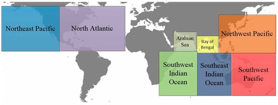
Figure 1.
Locations of tropical cyclones (TCs) and their basins.
2.2. Data Description
2.2.1. HY-2A Microwave Scatterometer
Microwave scatterometers can offer wind data of the sea surface (wind direction and wind speed). Quick Scatterometer (QuikSCAT) This has proven to be a very effective scatterometer that can obtain sea surface wind speeds with high accuracy [27,28], but this has not been available since 2009. Haiyang-2A (HY-2A) is the first altimetry and scatterometry satellite project of the China National Space Administration (CNSA), and it is dedicated to the studies of physical oceanography and geodesy. The Ku-band scatterometer is carried on HY-2A. Quantitative analysis shows the effectiveness of HY-2A sea surface wind field observations, and its advantages for typhoon monitoring [29]. Wind speeds and directions that are derived from HY-2A are accurate under medium and low wind speeds [30], though it is easily saturated at high wind speeds (>30 m/s). HY-2A satellite microwave scatterometer data can be obtained through the application of the National Satellite Ocean Application Service (NSOAS). Figure 2a is a HY-2A observation of Typhoon Fitow.
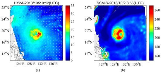
Figure 2.
Satellite observation of Typhoon Fitow (1323) in 2 October 2013, (a) HY-2A, and (b) SSMIS 19 GHz H-polarization.
2.2.2. SSMIS Microwave Radiometer
A microwave radiometer sensor is mounted onto HY-2A, but the radiometer data quality accuracy is lower than that of the microwave scatterometer. Therefore, a microwave radiometer with the closest possible matching time to the HY-2A transit time is needed. The HY-2A microwave scatterometer crosses the equator time onto its descending node at 6:00 local time, and on its ascending node at 18:00 local time. Therefore, a sensor that crosses the equator time at around 6:00, or 18:00 local time, is a priority when choosing a microwave radiometer. Therefore, the F17 SSMIS, carried onboard the Defense Meteorological Satellite Program (DMSP) satellites, was selected.
SSMIS is a seven-channel passive microwave radiometer operating at four frequencies (19.35, 22.235, 37.0, and 91 GHz) and dual-polarization (except at 22.235 GHz which is V-polarization only) [31,32]. SSMIS data are available through the NOAA Data Center’s Comprehensive Large Array-data Stewardship System (CLASS). Figure 2b is an SSMIS 19 GHz H-polarization observation of Typhoon Fitow.
2.2.3. Best-Track Data
Aircraft reconnaissance obviously provides the most accurate observations [33]. However, the global aircraft reconnaissance program has been inactivate since 1987, except for in the Atlantic Basin to the west of 55°W [34]. Although, a few dropsondes have been launched from aircraft reconnaissance flights during Pacific Asian Regional special observation campaigns, there is an insufficient number of TC cases for a statistically significant validation of the method using dropsondes alone. The best track intensities are initially calculated by using DT methods, and then modified by other observations such as aircraft reconnaissance, station, and ship weather reports, and Doppler radar. Thus, the best track intensity data are the only available references at present in the Northwest Pacific regions. The China Meteorological Administration (CMA) best-track datasets [35] were ultimately chosen as the validation data for this study. This best-track data can provide the location and intensity of TCs every six hours. Among the CMA best-track data, there are six types of TC intensity grades: Tropical depression (TD, 10.8–17.1 m/s), tropical Storm (TS, 17.2–24.4 m/s), severe tropical storm (STS, 24.5–32.6 m/s), typhoon (TY, 32.7–41.4 m/s), severe typhoon (STY, 41.5–50.9 m/s), and super typhoon (Super TY, ≥51.0 m/s).
The data from 2012–2017 were selected for model training and validation. Above all, HY-2A microwave scatterometer and SSMIS microwave radiometer data were matched according to the satellite overpass time difference. When collocating the satellite observations with the best track data, we used a time-varying criterion based on the TC intensity variation. The basic idea of this scheme is that we relax the restrictions for TCs with stable intensity and set more strict requirements for TCs with rapid intensity changes. There are three thresholds of overpass time difference: 10 min, 30 min, and 60 min. If the variation in the maximum-sustained wind (MSW) is greater than 5 m/s during the 6-hour interval of the nearest best track record time, the threshold of the overpass time difference between HY-2A and SSMIS is 10 min. If the variation in the MSW is less than 5 m/s, the threshold of the overpass time difference is 30 min. If there is no change in the MSW, the threshold is set to 60 min. This strategy brings us more matchup data, and reduces the impact of the overpass time difference on the estimated MWS. Later, the referenced MWS is linearly interpolated from the best track data, according to overpass time of SSMIS and HY-2A. For example, the overpass time of SSMIS and HY-2A are 6:10 (UTC), 6:20 (UTC), respectively. The intensity of TC corresponding to 6:15 (UTC) serves as our reference intensity. The intensity of 6:15 (UTC) is linearly interpolated according to the data values corresponding to the best track 6:00 (UTC) and 12:00 (UTC).
Lastly, 406 valid satellite-observed data contained in 119 TCs were selected. Among them, 261 satellite-observed data in 96 TCs are used as training sample data, and the other 145 data are used as test data (as shown in Table 1).

Table 1.
Information for the training data and test data.
3. Methodology
3.1. Relationship between the Satellite-Observed Parameters and the Maximum Wind Speed
In reference to Cecil and Zipser [36], the TB parameters of the SSMIS microwave radiometer and sea surface wind speed (SSW) parameters of HY-2A microwave scatterometer in concentric circles and annuli from the TC center were calculated, and then compared with the MSW using the CMA TC best track data. TB parameters are computed for each TB of 19, 22, 37, and 91 GHz over the ocean.
Similar to Hoshino et al. [17], we used two ways for the selection of coverage area when calculating each parameter. One way is a concentric circle, with different radii every 0.25° from 0.5° to 2.5°. Another way is an annuli enclosed by circles every 0.25°, such as annulus with a 1° inner radius and 1.25° outer radius (Figure 3). The center of the TC is set as the center of the circle, and it can be obtained by interpolation of the 6-hourly best track data. It should be noted that the different sizes of TCs and the eyewall replacement cycles may cause some intensity estimation errors. Therefore, the sizes of tropical cyclones and eyewall replacement cycles should be considered in future work. Then, the maximum, minimum, mean, and standard deviation (STD) of TB and SSW, and the ratio of pixels over the threshold (RAPT) of TB are computed in the computation coverage area. For RAPT, the minimum and maximum threshold temperatures for each frequency channel are 180 K and 270 K, respectively. There are, in total, 1785 parameters that are calculated in this process, so we formulated unified rules to name them. For the TB parameters obtained by SSMIS microwave radiometer, frequency, and polarization are first displayed (for instance, TB19H for horizontal polarized TB of 19 GHz). Then, the parameter type (MAX, MIN, MEAN, STD, MAX-MIN, and MAX-MEAN) was displayed (TB19H_MEAN). Lastly, a type of computation coverage (A or C) and radius follows. Computational regions are written as ‘A’ to represent annuli, followed by inner radius and outer radius for annuli (Axxxxxx, the first three x (xxx) are used for the position of the inner circle, the next three x (xxx) are for the position of the outer circle., i.e., TB19H_MEAN_A100125 represents an annulus whose inner radius is 1.0° and outer radius is 1.25°), and ‘C’ to represent a concentric circle, followed by the radius of the circle (Cxxx, 3 x (xxx) is used for circle radius, i.e., TB19H_MEAN_C100 represents a circle whose radius is 1.0°). For the SSW parameters obtained by the HY-2A microwave scatterometer, because they do not have as much frequency polarization information, they do not have a first step in naming rules like TB parameters do (SSW_MEAN_A100125 or SSW_MEAN_C100).
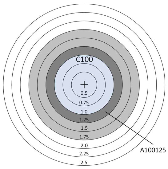
Figure 3.
An example of how the calculation regions for parameters are named. The circles are concentric circles whose radii represent every 0.25° latitude from 0.5° to 2.5° latitude. The cross is the center of the TC. C100 represents a concentric circle; the radius is 1°. A100125 represents the annuli whose inner radius is 1.0° and the outer radius is 1.25° (adapted from Hoshino & Nakazawa, 2007 [17]).
3.1.1. TB Parameters
In all, 1680 TB parameters were computed. In this section, the correlations between the TB parameters and TC intensity will be analyzed. The relationship between the single parameter of TB and the MSW of TC was analyzed by regression analysis, and then the Root Mean Square Error (RMSE) between the estimated and the best track MSW was calculated. The correlation coefficients between all of the parameters and the MSW of TC was calculated, and a significant horizontal t-test was conducted for the correlation coefficients.
The 10 highest correlated TB parameters with the maximum wind speeds for the best CMA tracks are shown in Table 2. The correlation coefficients and RMSEs are also given in the table. The highest correlated parameters were for TB19H_MIN_C100. The highest correlation coefficient was 0.84, and the RMSE was 6.67 m/s.
Table 2.
The highest correlated brightness temperature (TB) parameters.
The following conclusions can be inferred from Table 2:
There is a tendency for the parameters of 19, 22, and 37 GHz channels to give higher correlations with the TC maximum wind speed. The high frequency band reaches saturation when the cloud liquid water path is greater than 0.3 mm [37], while the cloud liquid water path in the eyewall of TC is between 0 and 0.5 mm [38]. Lower frequencies are less sensitive to the path of liquid water in clouds within this range. With the decreased sensitivity to the atmosphere, these channels will provide more information about the surface, and therefore lower frequencies could have higher correlations with the maximum wind speed.
The best correlated parameters for all frequencies are MIN and a few RAPT, but not MAX. MAX brightness temperature will be very high when there are more precipitation particles in a small area of TC, but this does not represent the overall intensity of TC [39]. Also, with the increase of precipitation intensity, different frequencies will have different degrees of saturation. MIN informs that all other points are larger than this number, and RAPT indicates the ratio of an active area, and hence it may be a more appropriate indicator to represent the TC intensity.
The parameters in the surrounding region (0.75–1.25° away from the TC center, especially 1°) tend to give higher correlations with the TC intensity. It is inferred that the intensity of the TC would be close to the radius of maximum wind speed. TC intensity estimates using a fixed annulus or circle could be impacted by TC eye size [39], so we should consider the sizes of the eyes, or the TCs in the future work.
The test dataset in Table 1 was used to verify the performance of only using TB19H_MIN_C100 parameter. The results of the validation are shown in Figure 4. The horizontal axis is the maximum wind speed that is estimated by the TB parameter model, and the vertical axis is the CMA TC best track intensity data. The R2 of the verification result for the test dataset was 0.76, the RMSE was 6.97 m/s, the MAE was 5.50 m/s, and the bias was −1.78 m/s. Figure 4b,c show the differences between the TB parameter model-estimated TC intensity and the CMA best-track data in two subgroups. Figure 4b relates to lower-intensity TCs, i.e., tropical depressions, tropical storms, and severe tropical storms. Figure 4c relates to typhoons, severe typhoons, and super typhoons.
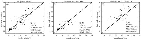
Figure 4.
Scatter plot of the maximum wind speed between the estimated results, using the TB19H_MIN_C100 parameter-only model and the China Meteorological Administration (CMA) best-track data. (a) All of the testing data. (b) Subgroup testing data of tropical depression (TD), tropical storm (TS), and severe tropical storm (STS). (c) Subgroup testing data of typhoon (TY), severe typhoon (STY), and super typhoon (Super TY).
3.1.2. SSW Parameters
In total, 105 SSW parameters were computed. In this section, the correlation between the SSW parameters and TC intensity will be analyzed. The relationship between the single parameter of SSW and the MSW of TC was analyzed by regression analysis, and then the RMSE between the estimated and the best-track MSW was calculated. The correlation coefficients between all of the parameters and the MSW of TC were calculated, and a significant horizontal t-test was conducted for the correlation coefficient.
The highest 15 correlated SSW parameters, correlation coefficients, and RMSEs with the CMA best tracks are shown in Table 3. The highest correlated parameter was for SSW_MEAN_C100. The highest correlation coefficient was 0.83, and the RMSE was 7.09 m/s.
Table 3.
The highest correlated sea surface wind (SSW) field parameters.
From Table 3, the following conclusions can be inferred:
The most closely correlated parameter for all radii is MEAN (and a few MIN). MEAN is computed over the entire corresponding region, and MIN describes that all other points are larger than this number; hence, it may be a more appropriate indicator to represent the TC intensity.
The parameters in the surrounding regions (0.75–1.5° away from the TC center) tended to give higher correlations with the CMA best-track data. We speculate that this reason is related to the radius of the wind circle. For most TCs, the radius of the Beaufort wind force 10 cyclone (24.5–28.4 m/s) is 50–100 km, and that of the wind force 12 (32.7–36.9 m/s) cyclone is 100–150 km.
The test dataset in Table 1 were used to verify the performance from using only the SSW_MEAN_C100 parameter. The results of the validation are shown in Figure 5. The horizontal axis is the maximum wind speed, as estimated by the SSW parameter model, and the vertical axis is the CMA TC best-track intensity data. The R2 of the verification result for the test dataset is 0.70, the RMSE is 7.84 m/s, the MAE is 6.11 m/s, and the BIAS is −1.49 m/s. Figure 5b,c shows the differences between the SSW parameter model-estimated TC intensity, and the CMA best-track data in two subgroups. Figure 5b relates to lower-intensity TCs, i.e., tropical depressions, tropical storms and severe tropical storms. Figure 5c relates to typhoons, severe typhoons, and super typhoons.
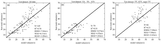
Figure 5.
Scatter plot of the maximum wind speed between the estimated results, using the SSW_MEAN_C100 parameter-only model, and the CMA best-track data. (a) All of the testing data. (b) Subgroup testing data of the TD, TS, and STS. (c) Subgroup testing data of TY, STY, and super TY.
3.2. Estimation of the Maximum Wind Speed using Selected Parameters
As described in the above section, it is shown that we can estimate the maximum wind speed by using a single parameter, with a certain accuracy (with 6.7–7.8 m/s RMSEs). However, including more predictors and using linear regression techniques could improve the estimation of TC intensity [40,41]. A stepwise regression method was used to select the most useful predictors from all of the above-mentioned 1785 parameters. Finally, 15 parameters were selected as follows. TB19H_MIN_C100, SSW_MIN_C100, TB19H_RAPT250_C075, SSW_MAX_C250, TB37H_RAPT210_C075, TB19H_RAPT_270_A225250, TB22V_RAPT270_A125150, TB37H_MAX_A125150, PCT92_MAX_C125, PCT92_MAX_C100, TB37V_RAPT260_C075, TB37H_RAPT180_A125150, TB37H_MIN_C100, PCT92_MAX_A150175, and SSW_MEAN_C100.
PCT (polarization-corrected temperature) is the parameter that is proposed by Spencer et al. [42], which represents the radiation eliminating the radiation from ocean using polarization diversity, and is calculated as:
where is the TB for the vertically polarized channel, and is that of the horizontally polarized channel at 85 GHz of the SSM/I. In this paper, we used PCT at 92 GHz of the SSMIS as candidate parameters.
However, the number of variables does not correspond to “the more the better” in linear regression. Figure 6 shows the dependence of R2 and RMSE with an increase in variable numbers. From Figure 6, we can conclude that when the number of parameters was six, the minimum RMSE and maximum R2 values occurred. Therefore, these six parameters were chosen as the final regression variables, and the proposed TC intensity estimation model is as follows:
where, Vmax is the maximum wind speed of TC, SSW_MIN_C100 is the minimum wind speed within 1 degree of distance from the TC center, TB19H_RAPT250_C075 is the percentage of pixels with TB19GHz, H-pol larger than 250 K within 0.75 degrees of distance from the TC center, SSW_MAX_C250 is the maximum wind speed within 2.5 degrees of distance from the TC center, TB37H_RAPT210_C075 is the percentage of pixels, with TB37GHz, H-pol being larger than 210 K within 0.75 degrees from the TC center, TB22V_RAPT270_A125150 is the percentage of pixels, with TB22GHz, V-pol being larger than 270 K between 1.25 degrees and 1.5 degrees from the TC center, and TB37H_MIN_C100 is the minimum TB of 37 GHz horizontal polarization within 1 degree of distance from the TC center.
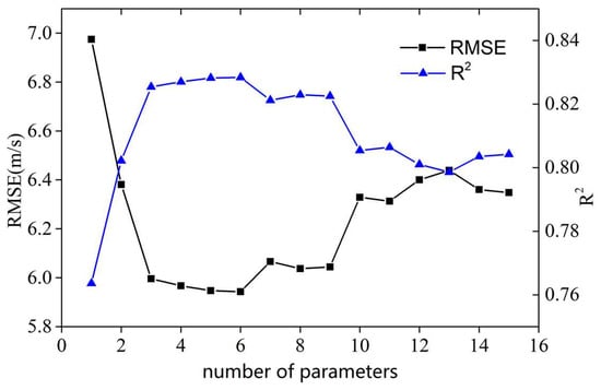
Figure 6.
Parameters of different numbers used to determine the best estimation model. The X-axis is the number of parameters, the left Y-axis is RMSE, and the right Y-axis is R2.
4. Experimental Results
4.1. Model Verification
4.1.1. Comparison with the TC Best-Track Wind Speed Estimates
The training dataset and test dataset in Table 1 were used to verify the performance of our estimation method. The results of the validation are shown in Figure 7. The horizontal axis is the maximum wind speed estimated by the proposed model, and the vertical axis is the CMA TC best-track intensity data. Unexpectedly, the accuracy of the training dataset is higher, but there was little difference between the training dataset and test dataset when the intensity of TC is TY, STY, and super TY. The R2 of our method verification result for the training dataset was 0.89, the RMSE was 4.19 m/s, the MAE was 3.20 m/s, and the BIAS was −0.008 m/s. The R2 of our method verification result for test dataset was 0.83, the RMSE was 5.94 m/s, the MAE was 4.62 m/s, and the BIAS was −0.43 m/s. Figure 7b–f shows the differences between model-estimated TC intensity and the CMA best track data in four subgroups. Figure 7b,e relate to lower-intensity TCs, i.e., tropical depressions, tropical storms, and severe tropical storms. Figure 7c,f relate to typhoons, severe typhoons, and super typhoons. Compared with Figure 4 and Figure 5, we can see from Figure 7 that using combined HY-2A and SSMIS is better than the use of either HY-2A or SSMIS separately.
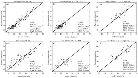
Figure 7.
Scatter plot of the comparison between the estimated maximum wind speed and the CMA best-track data. The solid line is y = x. (a) all data for training dataset, (b) TD, TS and STS for the training dataset, (c) TY, STY and the super TY for training dataset, (d) all data for test dataset, (e) TD, TS, and STS for the test dataset, (f) TY, STY, and super TY for test dataset.
4.1.2. Comparison with the Passive-Only Model
In order to test the usefulness of the include active observations into the TC intensity estimation model, the Hoshino et al. [17] method was chosen to compare with the proposed model. The selected parameters, the coefficients and RMSEs of the 10 candidates of regression equations are shown in Equation (3) and Table 4.
Table 4.
The parameters, coefficients, R2, and RMSE of the candidates for the regression equation.
As shown in Table 4, the average RMSE of the Hoshino model was 6.57 m/s. This RMSE is larger than the estimation of the proposed method, comparing with both the training dataset or the test dataset (see Figure 7a,d). It is also indicated that synergy by using active and passive microwave observations can obtain better estimation results than by only using passive observation as model predictors.
4.1.3. Comparison with Other Existing Models
Following Jiang et al. [21], a comparison with several existing algorithms for estimating TC intensities was made. Their RMSE and MAE are shown in Table 5. It is worth pointing out that we did not apply these existing methods to the same dataset used in this study, to calculate their errors. The statistical numbers listed in this table are all calculated from different data in different regions. It is worth mentioning that the smaller RMSE of the proposed method shown in Table 5 does not mean that this method is superior to others. It is only compared with the best track data, but not with an independent observation, like most of the other methods listed in the table.
Table 5.
Comparison of the model-estimated TC intensities with previously developed techniques using the statistical values of RMSE and MAE.
4.1.4. The Impact of Overpass Time Difference on Model Estimation
Since the HY-2A scatterometer and SSMIS radiometer have different overpass times when collecting the dataset used in this study, it needs to further analyze its impact on the estimated TC intensity. We calculated the RMSEs between the MSW that was estimated by the proposed model and the CMA best track data at 5 min intervals for the overpass time difference (see Figure 8).
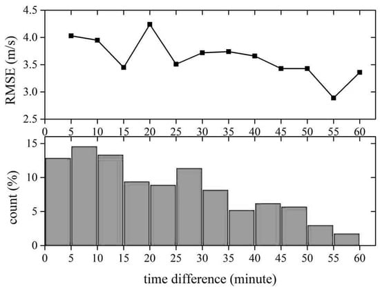
Figure 8.
RMSE values of the proposed model calculated at 5 min intervals of overpass time difference (upper panel); and the percentage of the sample number at each bin (lower panel).
As shown in Figure 8, the RMSEs did not increase as the time difference became larger. Most of the RMSEs were in the range of 3.5 to 4 m/s. The smallest RMSE occurred at the 55 min time difference bin, and it was probably due to the small sample size of the high wind conditions. This results indicate that the data matching scheme used in this study was effective; the errors introduced by these time differences had no significant effect on the estimated MSW.
4.2. Case Studies
4.2.1. Typhoon Tembin (1214)
The time-series plot of the maximum wind speed for Typhoon Tembin (1214) is shown in Figure 9a. In this figure, the green dot indicates the estimated maximum wind speed by the proposed regression model, and the red line showed the maximum wind speed by the CMA best-track data. This figure shows that the variations of the maximum wind speed estimated by the regression model has good consistency with the maximum wind speed by the TC best-track data. However, in individual cases, the estimated intensity of TC will sometimes be underestimated or overestimated. Figure 9b is the time-series plot of the maximum wind speed for Super Typhoon Noru (1705). We can see that the tendency of intensity change corresponded reasonably well with the maximum wind speed by the TC best-track data, but there were two clearly underestimated values in the initial stage and in the maximum wind speed stage.
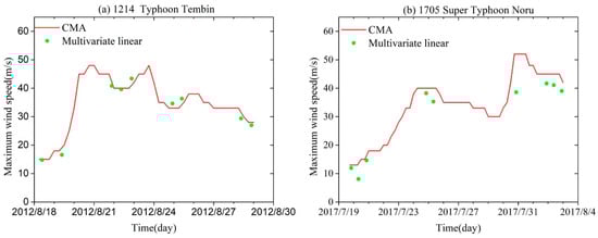
Figure 9.
Time series plot of the maximum wind speed estimated by the regression model, and the best track data for (a) Typhoon Tembin (1214) and (b) Super Typhoon Noru (1705).
We can observe that in the weak TC stages (<15 m/s), the outputs of the proposed method tended to underestimate the maximum wind speeds (Figure 7e and Figure 9). The possible reason for this was the difficulty in positioning the TC center, due to an unorganized cloud pattern. Figure 10 shows the SSMIS and HY-2A images of Super Typhoon Noru (1705) at 20 July 2017 (the early stage). The maximum wind speed estimated by the regression model was 8.1 m/s, but the maximum wind speed in the CMA best-track data was 13.6 m/s. This may be related to the accuracy in the positioning of the center, and the unorganized patterns.
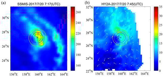
Figure 10.
Images of Super Typhoon Noru (1705) at 20 July 2017, during the early stages of development,(a) SSMIS, (b) HY-2A. The estimated maximum wind speed was 8.1 m/s, but the CMA best-track data was 13.6 m/s. The cross symbol is the center of Noru. The radii of the circles from inside to outside are 0.5°, 0.75°, 1°, and 1.25°, respectively.
4.2.2. Typhoon Noru (1705)
In Figure 9, we also noted that our method tended to underestimate the maximum wind speeds when the best track data was about 40 m/s. Figure 11 shows the SSMIS and HY-2A images of Super Typhoon Noru (1705) at 30 July 2017 (the mature stage). The maximum wind speed estimated by the regression model was 45.98 m/s, but the maximum wind speed in the CMA best-track data was 52 m/s. In the regression model, SSW_MAX_C250 was 28.54 m/s. At the same intensity, we found that in the previous image, SSW_MAX_C250 value was 38.5 m/s. Meanwhile, we analyzed that the value of the Advanced Scatterometer (ASCAT) wind field data on this day was 28.23 m/s. Also, the precipitation rate obtained by the GPM was above 450 mm/day. Therefore, we inferred that this error was probably due to the wind speed retrieval error caused by heavy rainfall.
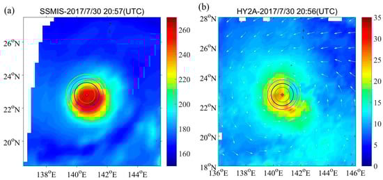
Figure 11.
Images of Super Typhoon Noru (1705) at 30 July 2017, during the mature stage of development, (a) SSMIS, (b) HY-2A. The estimated maximum wind speed was 45.98 m/s, but the CMA best-track data was 52 m/s. The cross symbol is the center of Noru. The radii of the circles from inside to outside are 0.5°, 0.75°, 1°, and 1.25°, respectively.
5. Discussion
The sea surface wind field can be derived directly from the microwave scatterometer. However, there was a large error under high wind speed conditions, which makes it impossible to directly determine the typhoon intensity from scatterometer observations. However, the scatterometer data can still provide useful information when estimating the TC intensity. In our study, when choosing the model predictors, we consider different radius ranges, and we take into account the maximum, minimum, and average values of the wind speed obtained from HY-2A scatterometer. The results (as shown in Table 3) show that parameters, such as the mean wind speed near the inner center of TC are much correlated with TC intensity. Therefore, when the wind speed is higher than 30 m/s, the active microwave observations will still add some useful information. This is why we want to introduce the active microwave observations into the TC intensity estimation model.
The overall accuracy of our estimated model has been improved, compared with the method of using the microwave radiometer alone [18]. But there are still large errors in some cases. Here are several possible reasons. (1) Errors in the determination of the cyclone centers, because of unorganized clouds with the TC in its earlier or dissipation stage. In the future, we will need to improve the accuracy of TC center determination, especially in the early or dissipation stage. Automated techniques such as the Automated Rotational Center Hurricane Eye Retrieval [15,49] method might be of benefit for center determination. (2) The time difference between the overpass time of HY-2A and F17 will introduce errors into the model estimates. Adopting more restrictive criteria when matching the training dataset could reduce this error. (3) The asymmetry of cyclone shape has an influence on our circular hypothesis. Also, to solve the problem of asymmetry, we need to introduce asymmetric characteristic factors and other parameters to increase the stability of the model. (4) We used the radius of the TC center in the range of 2.5 degrees, so that the size of the TC also had a certain impact on our model. Therefore, we may consider the size of the TC as a parameter for future research. (5) One other possible source of error are the potential for lag in the intensity, especially during rapid intensification, where the satellite presentation leads the intensity by several hours. In follow-up work, we should take into account the occurrence of this rapid intensification.
In this paper, firstly, we selected 15 parameters from many parameters by the stepwise regression method. Three out of the 15 selected parameters were related to 92 GHz. In the proposed model, the optimal combination of six parameters was chosen, but there were no 92 GHz parameters. In the future, more feature parameters will be introduced, and we will try to use more complicated statistical methods to select the optimal combination of the feature parameters. Our feature parameters are selected for all stages of TC. Some parameters may be better for certain TC stages; therefore, one may consider different feature parameter combinations in different stages of TC in their new models.
The proposed model is developed based on observations of typhoons in the Northwestern Pacific Ocean. To further test whether it will still be useful to hurricanes in the Atlantic and East Pacific Oceans, we have collected more test data in these regions. Unlike the Northwestern Pacific, there are airborne observations for hurricanes. Aircraft reconnaissance data of the Atlantic basin, Northeast and North Central Pacific basin can be obtained from the National Hurricane Center (NHC) at its website (http://www.aoml.noaa.gov/hrd/data_sub/hurr.html). With the operational deployment of the Stepped Frequency Microwave Radiometer (SFMR), hurricane reconnaissance and research aircraft provide near real-time observations of the 10 ocean-surface wind-speed, both within and around tropical cyclones [50]. In total, 13 matchups were collected in 2014–2015 (see Figure 12 below). Since the matchups were too few to recalculate the model coefficients, we directly used the coefficients obtained from Northwest Pacific region. In Figure 12, we can see that the model-estimated TC intensities did not perform well compared to the aircraft reconnaissance data. The differences among the model-estimated MWS, best-track, and aircraft measurements were very large, with MAE > 12 m/s and RMSE ~8 m/s. Both were much worse than the performance in the Northwestern Pacific Ocean (as shown in Figure 7). Hurricanes and typhoons have some differences in their structure and formation mechanisms. It is indicated that the coefficients of the proposed model were more suitable for typhoons than for hurricanes. Thus, the coefficients of the proposed model need to be tuned with enough matchup samples before its application to TCs in basins other than the Northwestern Pacific Ocean. In addition, the current comparison among SSMIS-only, HY2A-only, and their combined methods is not very rigorous. Only one parameter was tested for the SSMIS-only and HY2A-only methods, and the one-parameter approach is not the best option for estimating the TC intensity. In the future, we will need to consider more comprehensive and solid comparisons between the proposed model and other estimation models, using more sufficient ground true data.
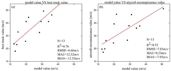
Figure 12.
Scatter plot of the comparison between the estimated maximum wind speed and the National Hurricane Center (NHC) best-track data and aircraft reconnaissance data in the Atlantic basin, and the Northeast and North Central Pacific basin. The solid line is the fitting line. (a) Proposed model vs best-track data (b) proposed model vs aircraft observations.
6. Conclusions
In this paper, a method to estimate TC intensity was developed, using SSMIS radiometer and HY-2A scatterometer data from the Northwest Pacific, from 2012 to 2017. First, we studied the correlation between the TB parameters, SSW parameters, and the MSW, to form the best-track data of the TCs. We found, for the SSMIS radiometer, that (1) the parameters of 19 GHz and 37 GHz channels give higher correlations with the TC MSW; (2) the horizontal polarization has a higher correlation than the vertical polarization at the same frequency; (3) the most well-correlated parameter for all frequencies is MIN; (4) the parameters in the surrounding regions (0.75–1.25° away from the TC center, especially 1°) tend to give higher correlations with the TC intensity. The highest correlation coefficient is 0.84, and the highest RMSE is 6.67 m/s. In addition, for HY-2A scatterometer, (1) the most well-correlated parameter for all radii is MEAN (and a few MIN); (2) the parameters for the surrounding regions (0.75–1.5° away from the TC center) tend to give higher correlations with the CMA best-track data. The highest correlation coefficient is 0.83, and the highest RMSE is 7.09 m/s.
Then, the TC intensity-estimated model was developed based on multiple linear regression, using selected parameters. We evaluated our estimated method by using independent verification data. The R2 of our verification is 0.83, the RMSE is 5.94 m/s, the MAE is 4.62 m/s, and the BIAS is −0.43 m/s. The estimated results of our model are therefore comparable to those of other algorithms.
On 25 October 2018, the HY-2B satellite was launched, as well as a subsequent series of HY-2 satellites, which formed an ocean dynamics satellite constellation to provide additional TC observation data. In the next five years, the Chinese HY-2C and FY-3E, which also carry radiometer and scatterometer equipment, will be launched. There will be more satellite data for both typhoons and hurricanes available to improve and implement the proposed method at that time.
Author Contributions
All authors have made great contributions to this article. Conceptualization, X.Y.; Formal analysis, K.X.; Methodology, X.Y., K.X.; Software, K.X., S.W.; Validation, K.X.; Writing—original draft, K.X., X.Y.; Writing—review & editing, K.X., X.Y.
Funding
This research was supported by the National Key R&D Program of China under Grant 2017YFB0502800, and in part, by the National Natural Science Foundation of China under Grant 41871268, and in part, by the Key Research and Development Program of Hainan Province under Grant ZDYF2017167.
Acknowledgments
The HY-2A microwave scatterometer data are provided by the National Satellite Ocean Application Service (NSOAS). The SSMIS microwave radiometer data are produced by Remote Sensing Systems, with support from NASA. Data are available at www.remss.com. The best-track data were obtained through the China Meteorological Administration (CMA). We are grateful to NSOAS, NOAA, and CMA for access to these data.
Conflicts of Interest
The authors declare no conflicts of interest.
References
- Tang, D.L.; Sui, G.; Lavy, G.; Pozdnyakov, D.; Song, Y.T.; Switzer, A.D. Typhoon Impact and Crisis Management; Springer: Berlin, Germany, 2014. [Google Scholar]
- Dvorak, V.F. Tropical cyclone intensity analysis and forecasting from satellite imagery. Mon. Weather Rev. 1975, 103, 420–430. [Google Scholar] [CrossRef]
- Dvorak, V.F. Tropical Cyclone Intensity Analysis Using Satellite Data; National Environmental Satellite, Data, and Information Service, National Oceanic and Atmospheric Administration, US Department of Commerce: Silver Spring, MD, USA, 1984; Volume 11.
- Velden, C.S.; Olander, T.L.; Zehr, R.M. Development of an objective scheme to estimate tropical cyclone intensity from digital geostationary satellite infrared imagery. Weather Forecast. 1998, 13, 172–186. [Google Scholar] [CrossRef]
- Olander, T.L.; Velden, C.S.; Turk, M.A. Development of the Advanced Objective Dvorak Technique (AODT)–Current progress and future directions. In Proceedings of the 25th Conference on Hurricanes and Tropical Meteorology, San Diego, CA, USA, 29 April–3 May 2002; pp. 585–586. [Google Scholar]
- Olander, T.L.; Velden, C.S. The advanced Dvorak technique: Continued development of an objective scheme to estimate tropical cyclone intensity using geostationary infrared satellite imagery. Weather Forecast. 2007, 22, 287–298. [Google Scholar] [CrossRef]
- Piñeros, M.F.; Ritchie, E.A.; Tyo, J.S. Objective measures of tropical cyclone structure and intensity change from remotely sensed infrared image data. IEEE Trans. Geosci. Remote Sens. 2008, 46, 3574–3580. [Google Scholar] [CrossRef]
- Piñeros, M.F.; Ritchie, E.A.; Tyo, J.S. Estimating tropical cyclone intensity from infrared image data. Weather Forecast. 2011, 26, 690–698. [Google Scholar] [CrossRef]
- Ritchie, E.A.; Valliere-Kelley, G.; Piñeros, M.F.; Tyo, J.S. Tropical cyclone intensity estimation in the North Atlantic Basin using an improved deviation angle variance technique. Weather Forecast. 2012, 27, 1264–1277. [Google Scholar] [CrossRef]
- Ritchie, E.A.; Wood, K.M.; Rodríguez-Herrera, O.G.; Piñeros, M.F.; Tyo, J.S. Satellite-derived tropical cyclone intensity in the north pacific ocean using the deviation-angle variance technique. Weather Forecast. 2014, 29, 505–516. [Google Scholar] [CrossRef]
- Zhang, C.-J.; Qian, J.-F.; Ma, L.-M.; Lu, X.-Q. Tropical Cyclone Intensity Estimation Using RVM and DADI Based on Infrared Brightness Temperature. Weather Forecast. 2016, 31, 1643–1654. [Google Scholar] [CrossRef]
- Lu, X.; Yu, H.; Yang, X.; Li, X. Estimating Tropical Cyclone Size in the Northwestern Pacific from Geostationary Satellite Infrared Images. Remote Sens. 2017, 9, 728. [Google Scholar] [CrossRef]
- Hawkins, J.D.; Lee, T.; Turk, F.; Richardson, K.; Sampson, C.; Kent, J. Mapping tropical cyclone characteristics via passive microwave remote sensing. In Proceedings of the 11th Conference on Satellite Meteorology and Oceanography, Madison, WI, USA, 15–18 October 2001. [Google Scholar]
- Wimmers, A.J.; Velden, C.S. Objectively determining the rotational center of tropical cyclones in passive microwave satellite imagery. J. Appl. Meteorol. Climatol. 2010, 49, 2013–2034. [Google Scholar] [CrossRef]
- Bankert, R.L.; Tag, P.M. An automated method to estimate tropical cyclone intensity using SSM/I imagery. J. Appl. Meteorol. 2002, 41, 461–472. [Google Scholar] [CrossRef]
- Bankert, R.L.; Cossuth, J. Tropical Cyclone Intensity Estimation via Passive Microwave Data Features. In Proceedings of the 32rd Conf. on Hurricanes and Tropical Meteorology, San Juan, Puerto Rico, 17–22 April 2016. [Google Scholar]
- Hoshino, S.; Nakazawa, T. Estimation of tropical cyclone’s intensity using TRMM/TMI brightness temperature data. J. Meteorol. Soc. Jpn. 2007, 85, 437–454. [Google Scholar] [CrossRef]
- Yang, S.; Hawkins, J.; Richardson, K. The improved NRL tropical cyclone monitoring system with a unified microwave brightness temperature calibration scheme. Remote Sens. 2014, 6, 4563–4581. [Google Scholar] [CrossRef]
- Zhou, X.; Yang, X.; Li, Z.; Yu, Y.; Bi, H.; Ma, S.; Li, X. Estimation of tropical cyclone parameters and wind fields from SAR images. Sci. China Earth Sci. 2013, 56, 1977–1987. [Google Scholar] [CrossRef]
- Zhang, G.; Li, X.; Perrie, W.; Hwang, P.A.; Zhang, B.; Yang, X. A Hurricane Wind Speed Retrieval Model for C-Band RADARSAT-2 Cross-Polarization ScanSAR Images. IEEE Trans. Geosci. Remote Sens. 2017, 55, 4766–4774. [Google Scholar] [CrossRef]
- Jiang, H.; Tao, C.; Pei, Y. Estimation of Tropical Cyclone Intensity in the North Atlantic and North Eastern Pacific Basins Using TRMM Satellite Passive Microwave Observations. J. Appl. Meteorol. Climatol. 2019, 58, 185–197. [Google Scholar] [CrossRef]
- Said, F.; Long, D.G. Determining selected tropical cyclone characteristics using QuikSCAT’s ultra-high resolution images. IEEE J. Sel. Top. Appl. Earth Obs. Remote Sens. 2011, 4, 857–869. [Google Scholar] [CrossRef]
- Liu, S.; Li, Z.; Yang, X.; Pichel, G.W.; Yu, Y.; Zheng, Q.; Li, X. Atmospheric frontal gravity waves observed in satellite SAR images of the Bohai Sea and Huanghai Sea. Acta Oceanol. Sin. 2010, 29, 35–43. [Google Scholar] [CrossRef]
- Shao, W.; Li, X.; Hwang, P.; Zhang, B.; Yang, X. Bridging the gap between cyclone wind and wave by C-band SAR measurements. J. Geophys. Res. Ocean. 2017, 122. [Google Scholar] [CrossRef]
- Yang, X.; Li, X.; Zheng, Q.; Gu, X.; Pichel, W.G.; Li, Z. Comparison of Ocean-Surface Winds Retrieved from QuikSCAT Scatterometer and Radarsat-1 SAR in Offshore Waters of the U.S. West Coast. IEEE Geosci. Remote Sens. Lett. 2011, 8, 163–167. [Google Scholar] [CrossRef]
- Chen, L.; Ding, Y. An Introduction to Typhoons in the Western Pacific Ocean; Science Press: Beijing, China, 1979. [Google Scholar]
- Stiles, B.W.; Dunbar, R.S. A neural network technique for improving the accuracy of scatterometer winds in rainy conditions. IEEE Trans. Geosci. Remote Sens. 2010, 48, 3114–3122. [Google Scholar] [CrossRef]
- Stiles, B.W.; Danielson, R.E.; Poulsen, W.L.; Brennan, M.J.; Hristova-Veleva, S.; Shen, T.-P.; Fore, A.G. Optimized tropical cyclone winds from QuikSCAT: A neural network approach. IEEE Trans. Geosci. Remote Sens. 2014, 52, 7418–7434. [Google Scholar] [CrossRef]
- Lin, M.; Zhang, Y.; Song, Q.; Xie, X.; Zou, J. Application of HY-2 Satellite Microwave Scattering Meter in Typhoon Monitoring in Northwest Pacific Ocean. Chin. Eng. Sci. 2014, 16, 46–53. [Google Scholar]
- Yang, X.; Liu, G.; Li, Z.; Yu, Y. Preliminary validation of ocean surface vector winds estimated from China’s HY-2A scatterometer. Int. J. Remote Sens. 2014, 35, 4532–4543. [Google Scholar] [CrossRef]
- Yan, B.; Weng, F. Intercalibration between special sensor microwave imager/sounder and special sensor microwave imager. IEEE Trans. Geosci. Remote Sens. 2008, 46, 984–995. [Google Scholar]
- Kerola, D.X. Calibration of Special Sensor Microwave Imager/Sounder (SSMIS) upper air brightness temperature measurements using a comprehensive radiative transfer model. Radio Sci. 2006, 41, 1–11. [Google Scholar] [CrossRef]
- Velden, C.; Harper, B.; Wells, F.; Beven, J.L.; Zehr, R.; Olander, T.; Mayfield, M.; Guard, C.C.; Lander, M.; Edson, R. The Dvorak tropical cyclone intensity estimation technique: A satellite-based method that has endured for over 30 years. Bull. Am. Meteorol. Soc. 2006, 87, 1195–1210. [Google Scholar] [CrossRef]
- Gray, W.M.; Neumann, C.; Tsui, T.L. Assessment of the role of aircraft reconnaissance on tropical cyclone analysis and forecasting. Bull. Am. Meteorol. Soc. 1991, 72, 1867–1884. [Google Scholar] [CrossRef]
- Ying, M.; Zhang, W.; Yu, H.; Lu, X.; Feng, J.; Fan, Y.; Zhu, Y.; Chen, D. An overview of the China Meteorological Administration tropical cyclone database. J. Atmos. Ocean. Technol. 2014, 31, 287–301. [Google Scholar] [CrossRef]
- Cecil, D.J.; Zipser, E.J. Relationships between tropical cyclone intensity and satellite-based indicators of inner core convection: 85-GHz ice-scattering signature and lightning. Mon. Weather Rev. 1999, 127, 103–123. [Google Scholar] [CrossRef]
- Lee, T.F.; Turk, F.J.; Hawkins, J.; Richardson, K. Interpretation of TRMM TMI Images of Tropical Cyclones. Earth Interact. 2002, 6, 1. [Google Scholar] [CrossRef]
- Weng, F.; Grody, N.C. Retrieval of cloud liquid water using the Special Sensor Microwave Imager. J. Geophys. Res. Atmos. 1994, 99, 25535–25551. [Google Scholar] [CrossRef]
- Yoshida, S.; Sakai, M.; Shouji, A. Estimation of tropical cyclone’s intensity using Aqua/AMSR-E data. Meteorol. Satell. Cent. Tech. Note 2009, 13–42. [Google Scholar]
- Olander, T.L.; Velden, C.S. Tropical cyclone convection and intensity analysis using differenced infrared and water vapor imagery. Weather Forecast. 2009, 24, 1558–1572. [Google Scholar] [CrossRef]
- Zhao, Y.; Zhao, C.; Sun, R.; Wang, Z. A Multiple Linear Regression Model for Tropical Cyclone Intensity Estimation from Satellite Infrared Images. Atmosphere 2016, 7, 40. [Google Scholar] [CrossRef]
- Spencer, R.W.; Hood, R.E.; Goodman, H.M. Precipitation Retrieval over Land and Ocean with the SSM/I: Identification and Characteristics of the Scattering Signal. J. Atmos. Ocean. Technol. 1989, 6, 254–273. [Google Scholar] [CrossRef]
- Demuth, J.L.; DeMaria, M.; Knaff, J.A.; Vonder Haar, T.H. Evaluation of Advanced Microwave Sounding Unit tropical-cyclone intensity and size estimation algorithms. J. Appl. Meteorol. 2004, 43, 282–296. [Google Scholar] [CrossRef]
- Demuth, J.L.; DeMaria, M.; Knaff, J.A. Improvement of Advanced Microwave Sounding Unit tropical cyclone intensity and size estimation algorithms. J. Appl. Meteorol. Climatol. 2006, 45, 1573–1581. [Google Scholar] [CrossRef]
- Kossin, J.P.; Knapp, K.R.; Vimont, D.J.; Murnane, R.J.; Harper, B.A. A globally consistent reanalysis of hurricane variability and trends. Geophys. Res. Lett. 2007, 34. [Google Scholar] [CrossRef]
- Knaff, J.A.; Brown, D.P.; Courtney, J.; Gallina, G.M.; Beven, J.L. An evaluation of Dvorak technique–based tropical cyclone intensity estimates. Weather Forecast. 2010, 25, 1362–1379. [Google Scholar] [CrossRef]
- Fetanat, G.; Homaifar, A.; Knapp, K.R. Objective tropical cyclone intensity estimation using analogs of spatial features in satellite data. Weather Forecast. 2013, 28, 1446–1459. [Google Scholar] [CrossRef]
- Pradhan, R.; Aygun, R.S.; Maskey, M.; Ramachandran, R.; Cecil, D.J. Tropical Cyclone Intensity Estimation Using a Deep Convolutional Neural Network. IEEE Trans. Image Process. 2018, 27, 692–702. [Google Scholar] [CrossRef] [PubMed]
- Wimmers, A.J.; Velden, C.S. Advancements in objective multisatellite tropical cyclone center fixing. J. Appl. Meteorol. Climatol. 2016, 55, 197–212. [Google Scholar] [CrossRef]
- Sapp, J.W.; Alsweiss, S.O.; Jelenak, Z.; Chang, P.S.; Carswell, J. Stepped Frequency Microwave Radiometer Wind-Speed Retrieval Improvements. Remote Sens. 2019, 11, 214. [Google Scholar] [CrossRef]
© 2019 by the authors. Licensee MDPI, Basel, Switzerland. This article is an open access article distributed under the terms and conditions of the Creative Commons Attribution (CC BY) license (http://creativecommons.org/licenses/by/4.0/).