Mapping Foliar Nutrition Using WorldView-3 and WorldView-2 to Assess Koala Habitat Suitability


Abstract
1. Introduction
2. Materials and Methods
2.1. Study Area
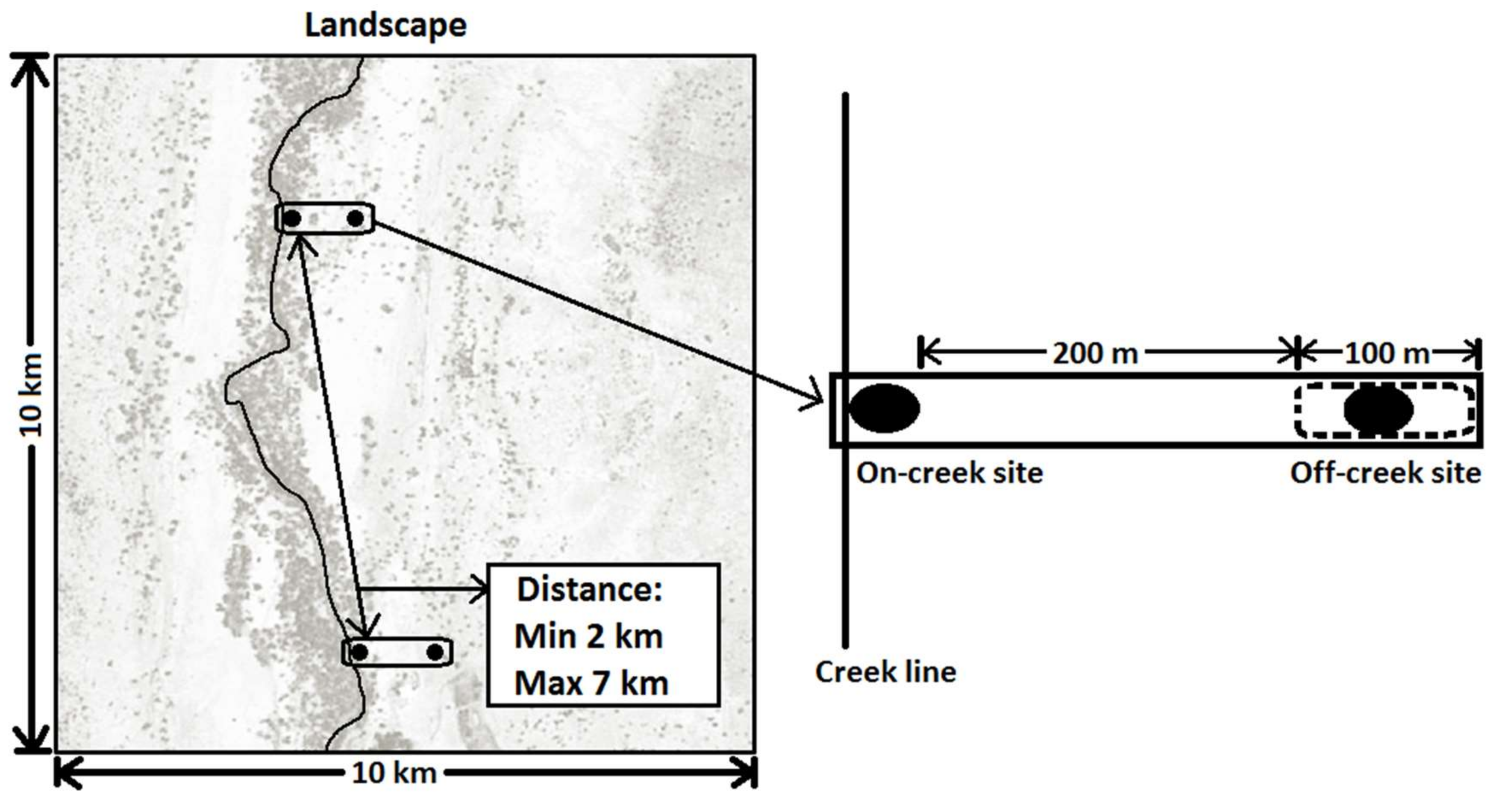
2.2. Survey Design
2.3. Field Sampling and Leaf Spectral Sampling
2.4. Foliar Chemical Analysis
2.5. WV3 Image Acquisition and Pre-Processing
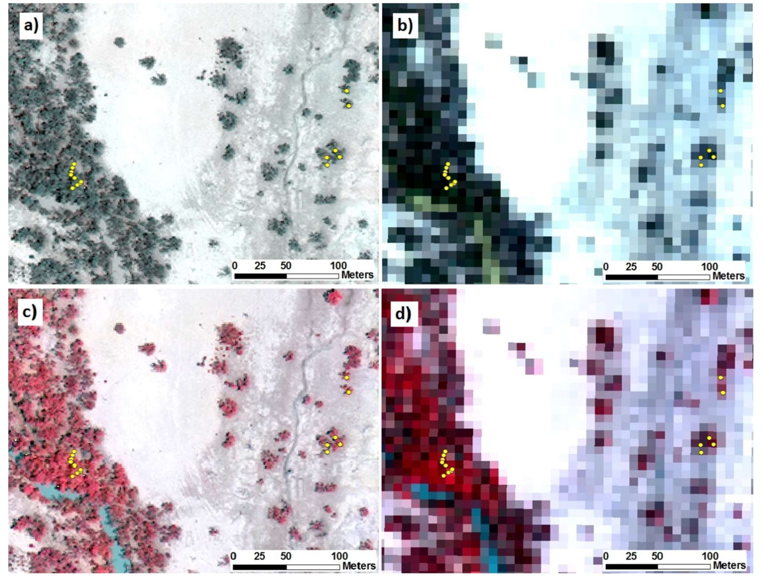
2.6. Collecting Image Spectra of Sampled Trees
2.7. Calculating and Assessing Spectral Indices
2.8. Mapping DigN with Selected Index
2.9. Application of DigN Mapping Method to WV2 Image
2.10. Associating Mapped DigN from WV2 Image with Koala Tree Use Data
3. Results
3.1. Laboratory Measures of Foliar Chemistry
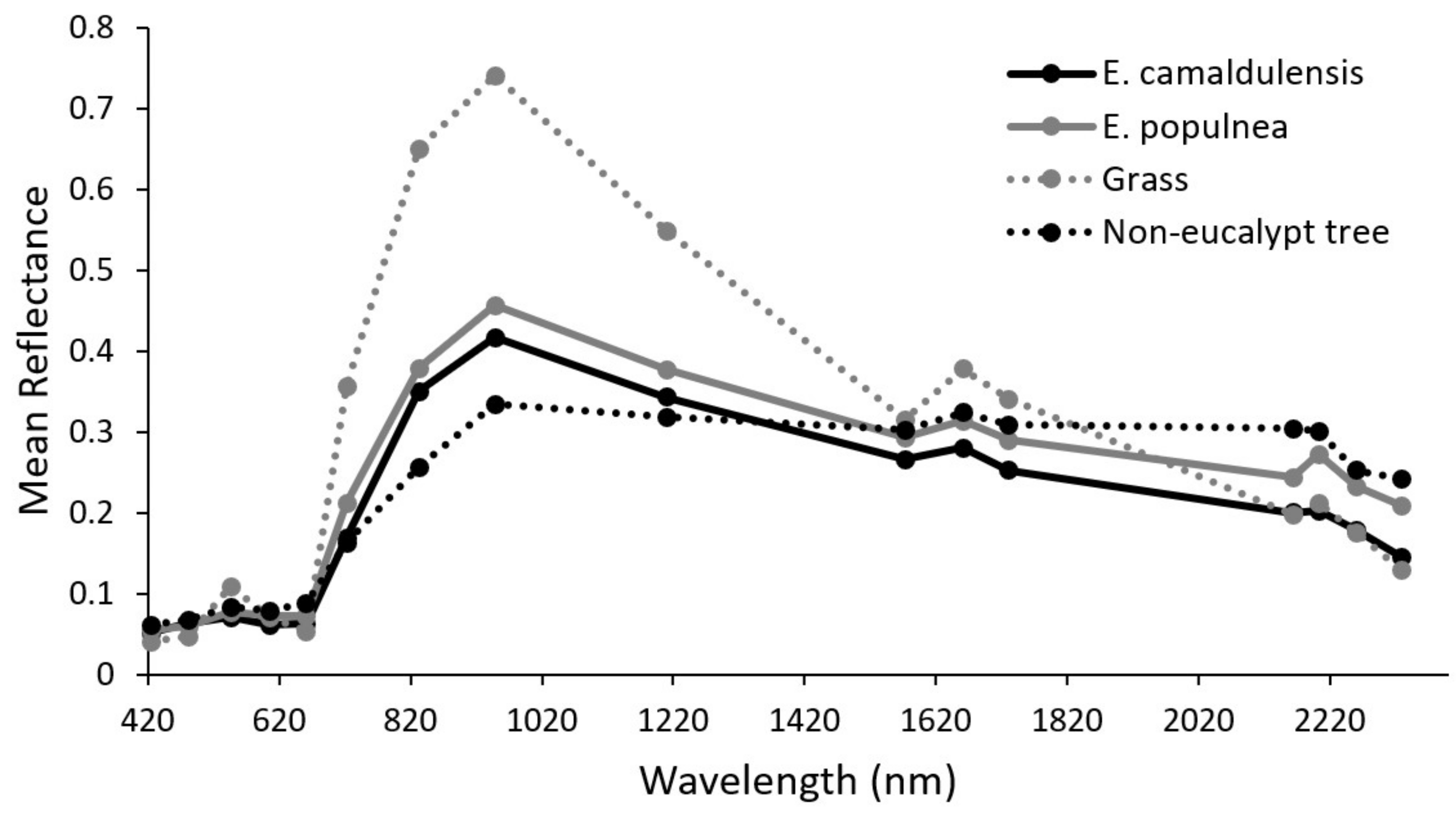
3.2. Estimation of DigN Concentration from Resampled ASD Spectra and WV3 Spectra
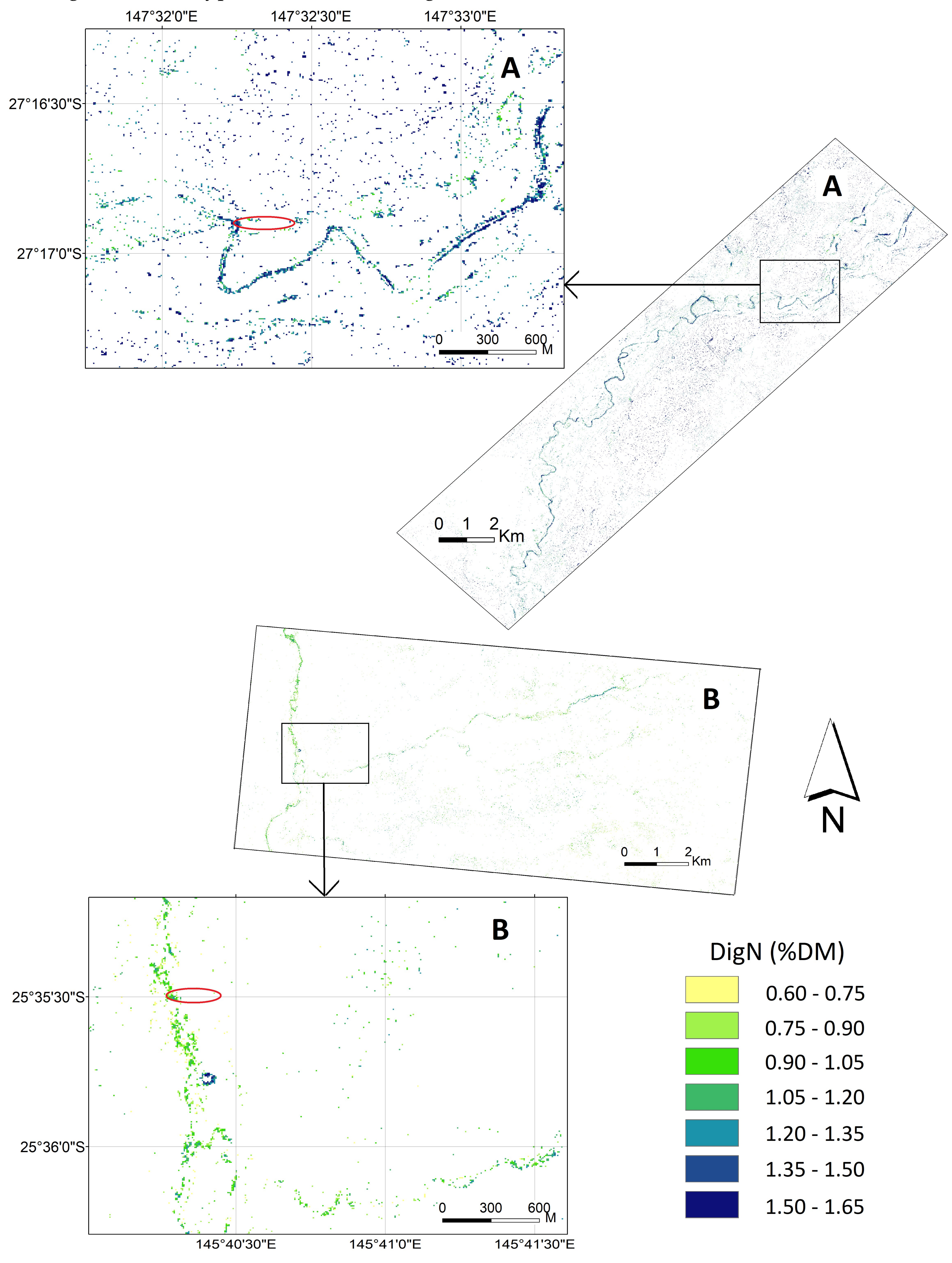
3.3. Mapping DigN with Selected Indices
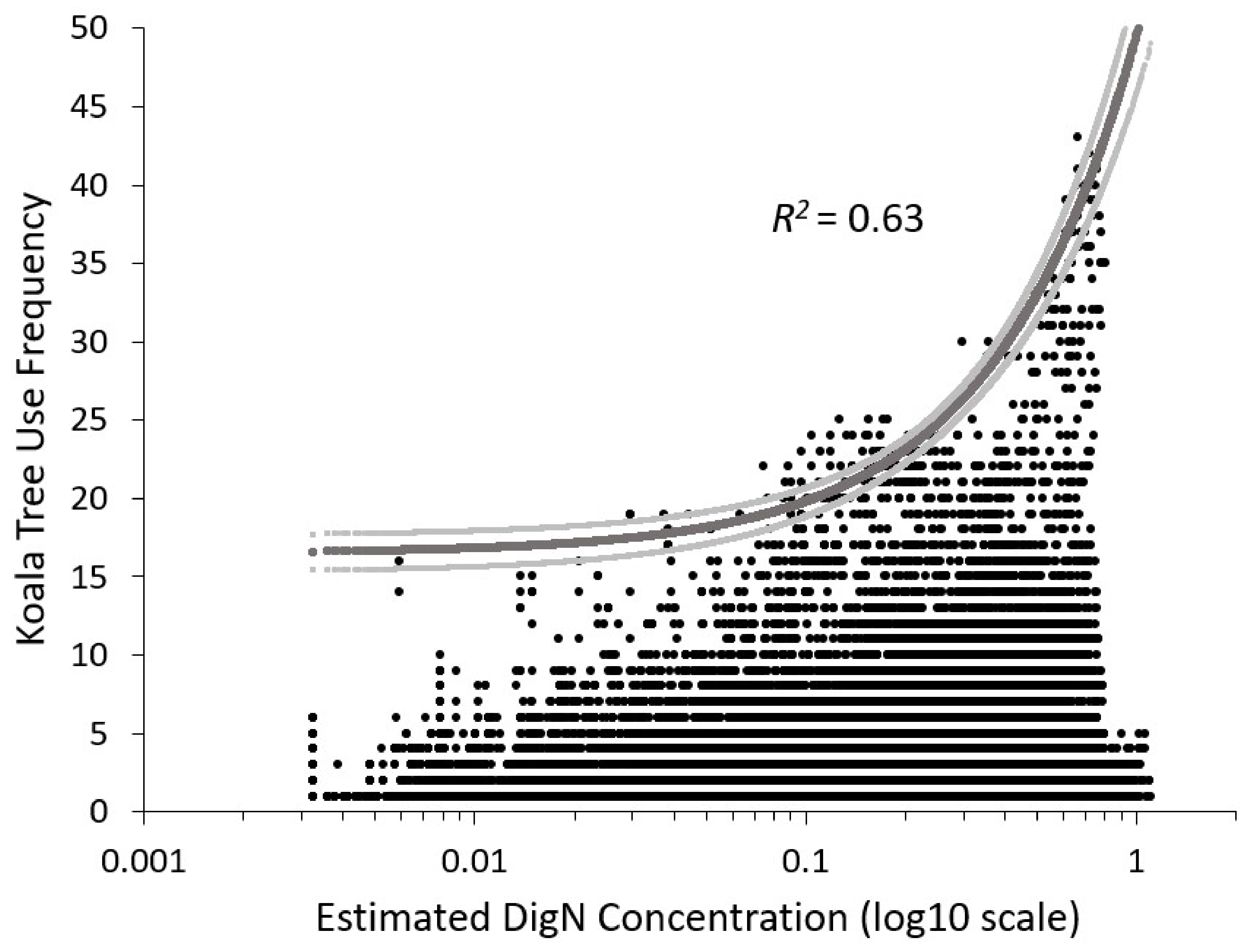
3.4. Relationship between Mapped DigN from WV2 Image with Koala Tree Use
4. Discussion
4.1. Spectral Indices to Estimate and Map Foliar DigN
4.2. Better Performance of WV3 7.5 m Spectra than 1.24 m Spectra
4.3. Mapped DigN to Evaluate Koala Habitat Suitability
5. Conclusions
Supplementary Materials
Author Contributions
Funding
Acknowledgments
Conflicts of Interest
References
- Environment Protection Authority. Koala Habitat Mapping Pilot: NSW State Forests. Available online: www.epa.nsw.gov.au (accessed on 12 May 2016).
- Callaghan, J.; McAlpine, C.; Thompson, J.; Mitchell, D.; Bowen, M.; Rhodes, J.; de Jong, C.; Sternberg, R.; Scott, A. Ranking and mapping koala habitat quality for conservation planning on the basis of indirect evidence of tree-species use: A case study of Noosa Shire, south-eastern Queensland. Wildl. Res. 2011, 38, 89–102. [Google Scholar] [CrossRef]
- GHD. South East Queensland Koala Habitat Assessment and Mapping Project. Available online: https://data.qld.gov.au/dataset/koala-planning-areas-version-1-2-south-east-queensland-data-package (accessed on 21 April 2018).
- Lunney, D.; Phillips, S.; Callaghan, J.; Coburn, D. Determining the distribution of koala habitat across a shire as a basis for conservation: A case study from Port Stephens, New South Wales. Pac. Conserv. Biol. 1998, 4, 186–196. [Google Scholar] [CrossRef]
- McAlpine, C.; Rhodes, J.; Callaghan, J.; Bowen, M.; Lunney, D.; Mitchell, D.; Pullar, D.; Possingham, H. The importance of forest area and configuration relative to local habitat factors for conserving forest mammals: A case study of koalas in Queensland, Australia. Biol. Conserv. 2006, 132, 153–165. [Google Scholar] [CrossRef]
- Moore, B.; Wallis, I.; Marsh, K.; Foley, W. The role of nutrition in the conservation of the marsupial folivores of eucalypt forests. In Conservation of Australia’s Forest Fauna; Lunney, D., Ed.; Royal Zoological Society of New South Wales: Mosman, Australia, 2004; pp. 549–575. [Google Scholar]
- Woinarski, J.; Burbidge, A. Phascolarctos Cinereus. Available online: https://www.iucnredlist.org/species/16892/21960344 (accessed on 5 June 2017).
- Marsh, K.; Moore, B.; Wallis, I.; Foley, W. Feeding rates of a mammalian browser confirm the predictions of a ‘foodscape’ model of its habitat. Oecologia 2014, 174, 873–882. [Google Scholar] [CrossRef] [PubMed]
- Moore, B.; Lawler, I.; Wallis, I.; Beale, C.; Foley, W. Palatability mapping: A koala’s eye view of spatial variation in habitat quality. Ecology 2010, 91, 3165–3176. [Google Scholar] [CrossRef] [PubMed]
- Munks, S.A.; Corkrey, R.; Foley, W.J. Characteristics of arboreal marsupial habitat in the semi-arid woodlands of northern Queensland. Wildl. Res. 1996, 23, 185–195. [Google Scholar] [CrossRef]
- Wu, H.; McAlpine, C.A.; Seabrook, L.M. The dietary preferences of koalas, Phascolarctos cinereus, in southwest Queensland. Aust. Zool. 2012, 36, 93–102. [Google Scholar] [CrossRef]
- Mertl-Millhollen, A.S.; Rambeloarivony, H.; Miles, W.; Kaiser, V.; Gray, L.; Dorn, L.; Williams, G.; Rasamimanana, H. The influence of tamarind tree quality and quantity on Lemur catta behavior. In Ringtailed Lemur Biology; Springer: New York, NY, USA, 2006; pp. 102–118. [Google Scholar]
- Simmen, B.; Tamaud, L.; Hladik, A. Leaf nutritional quality as a predictor of primate biomass: Further evidence of an ecological anomaly within prosimian communities in Madagascar. J. Trop. Ecol. 2012, 28, 141–151. [Google Scholar] [CrossRef]
- DeGabriel, J.; Wallis, I.; Moore, B.; Foley, W. A simple, integrative assay to quantify nutritional quality of browses for herbivores. Oecologia 2008, 156, 107–116. [Google Scholar] [CrossRef]
- DeGabriel, J.L.; Moore, B.D.; Foley, W.J.; Johnson, C.N. The effects of plant defensive chemistry on nutrient availability predict reproductive success in a mammal. Ecology 2009, 90, 711–719. [Google Scholar] [CrossRef] [PubMed]
- Skidmore, A.K.; Ferwerda, J.G.; Mutanga, O.; Van Wieren, S.E.; Peel, M.; Grant, R.C.; Prins, H.H.T.; Balcik, F.B.; Venus, V. Forage quality of savannas—Simultaneously mapping foliar protein and polyphenols for trees and grass using hyperspectral imagery. Remote Sens. Environ. 2010, 114, 64–72. [Google Scholar] [CrossRef]
- Eitel, J.; Long, D.; Gessler, P.; Smith, A. Using in-situ measurements to evaluate the new RapidEye™ satellite series for prediction of wheat nitrogen status. Int. J. Remote Sens. 2007, 28, 4183–4190. [Google Scholar] [CrossRef]
- Govender, M.; Chetty, K.; Naiken, V.; Bulcock, H. A comparison of satellite hyperspectral and multispectral remote sensing imagery for improved classification and mapping of vegetation. Water 2008, 34, 147–154. [Google Scholar]
- Youngentob, K.; Renzullo, L.; Held, A.; Jia, X.; Lindenmayer, D.; Foley, W. Using imaging spectroscopy to estimate integrated measures of foliage nutritional quality. Methods Ecol. Evol. 2012, 3, 416–426. [Google Scholar] [CrossRef]
- Adjorlolo, C.; Mutanga, O.; Cho, M.A. Estimation of canopy nitrogen concentration across C3 and C4 grasslands using Worldview-2 multispectral data. IEEE J. Sel. Top. Appl. Earth Obs. Remote Sens. 2014, 7, 4385–4392. [Google Scholar] [CrossRef]
- Zengeya, F.; Mutanga, O.; Murwira, A. Linking remotely sensed forage quality estimates from WorldView-2 multispectral data with cattle distribution in a savanna landscape. Int. J. Appl. Earth Obs. Geoinf. 2013, 21, 513–524. [Google Scholar] [CrossRef]
- Bagheri, N.; Ahmadi, H.; Alavipanah, S.K.; Omid, M. Multispectral remote sensing for site-specific nitrogen fertilizer management. Pesqui. Agropecu. Bras. 2013, 48, 1394–1401. [Google Scholar] [CrossRef]
- Boegh, E.; Houborg, R.; Bienkowski, J.; Braban, C.F.; Dalgaard, T.; Van Dijk, N.; Dragosits, U.; Holmes, E.; Magliulo, V.; Schelde, K.; et al. Remote sensing of LAI, chlorophyll and leaf nitrogen pools of crop- and grasslands in five European landscapes. Biogeosciences 2013, 10, 6279–6307. [Google Scholar] [CrossRef]
- Reyniers, M.; Vrindts, E. Measuring wheat nitrogen status from space and ground-based platform. Int. J. Remote Sens. 2006, 27, 549–567. [Google Scholar] [CrossRef]
- Zandler, H.; Brenning, A.; Samimi, C. Potential of space-borne hyperspectral data for biomass quantification in an arid environment: Advantages and limitations. Remote Sens. 2015, 7, 4565–4580. [Google Scholar] [CrossRef]
- Chemura, A.; Mutanga, O.; Odindi, J.; Kutywayo, D. Mapping spatial variability of foliar nitrogen in coffee (Coffea arabica L.) plantations with multispectral Sentinel-2 MSI data. ISPRS J. Photogramm. Remote Sens. 2018, 138. [Google Scholar] [CrossRef]
- Verma, N.; Lamb, D.; Reid, N.; Wilson, B. Comparison of canopy volume measurements of scattered eucalypt farm trees derived from high spatial resolution imagery and LiDAR. Remote Sens. 2016, 8, 388. [Google Scholar] [CrossRef]
- Davies, N.; Gramotnev, G.; Seabrook, L.; Bradley, A.; Baxter, G.; Rhodes, J.; Lunney, D.; McAlpine, C. Movement patterns of an arboreal marsupial at the edge of its range: A case study of the koala. Mov. Ecol. 2013, 1, 8. [Google Scholar] [CrossRef] [PubMed]
- Ream, B. Mapping Eucalypts in South-West Queensland: Answering the Question Can Fine Resolution Satellite Remote Sensing Be Used to Map Eucalypt Composition. Ph.D. Thesis, The University of Queensland, Brisbane, Australia, 2013. [Google Scholar]
- Seabrook, L.; McAlpine, C.; Rhodes, J.; Baxter, G.; Bradley, A.; Lunney, D. Determining range edges: Habitat quality, climate or climate extremes? Divers. Distrib. 2014, 20, 95–106. [Google Scholar] [CrossRef]
- Australian Government Bureau of Meteorology Climate Data Online. Available online: http://www.bom.gov.au/water/landscape/ (accessed on 31 October 2016).
- Rouse, J.; Harlan, J.; Haas, R.; Schell, J.; Deering, D. Monitoring the Vernal Advancement and Retrogradation (Green Wave Effect) of Natural Vegetation; Remote Sensing Center, Texas A&M University: College Station, TX, USA, 1974. [Google Scholar]
- Haboudane, D.; Miller, J.; Tremblay, N.; Zarco-Tejada, P.; Dextraze, L. Integrated narrow-band vegetation indices for prediction of crop chlorophyll content for application to precision agriculture. Remote Sens. Environ. 2002, 81, 416–426. [Google Scholar] [CrossRef]
- Herrmann, I.; Karnieli, A.; Bonfil, D.; Cohen, Y.; Alchanatis, V. SWIR-based spectral indices for assessing nitrogen content in potato fields. Int. J. Remote Sens. 2010, 31, 5127–5143. [Google Scholar] [CrossRef]
- Rondeaux, G.; Steven, M.; Baret, F. Optimization of soil-adjusted vegetation indices. Remote Sens. Environ. 1996, 55, 95–107. [Google Scholar] [CrossRef]
- Daughtry, C.; Walthall, C.; Kim, M.; de Colstoun, E.B.; McMurtrey, J. Estimating corn leaf chlorophyll concentration from leaf and canopy reflectance. Remote Sens. Environ. 2000, 74, 229–239. [Google Scholar] [CrossRef]
- Haboudane, D.; Miller, J.; Pattey, E.; Zarco-Tejada, P.; Strachan, I. Hyperspectral vegetation indices and novel algorithms for predicting green LAI of crop canopies: Modeling and validation in the context of precision agriculture. Remote Sens. Environ. 2004, 90, 337–352. [Google Scholar] [CrossRef]
- Marsh, K.J.; Moore, B.D.; Wallis, I.R.; Foley, W.J. Continuous monitoring of feeding by koalas highlights diurnal differences in tree preferences. Wildl. Res. 2014, 40, 639–646. [Google Scholar] [CrossRef]
- Cade, B.; Noon, B. A gentle introduction to quantile regression for ecologists. Front. Ecol. Environ. 2003, 1, 412–420. [Google Scholar] [CrossRef]
- Davies, N.; (The University of Queensland, Brisbane, Australia). Personal communication, 2014.
- Stalenberg, E.; Wallis, I.; Cunningham, R.; Allen, C.; Foley, W. Nutritional correlates of koala persistence in a low-density population. PLoS ONE 2014, 9, e113930. [Google Scholar] [CrossRef] [PubMed]
- Mutanga, O.; Adam, E.; Adjorlolo, C.; Abdel-Rahman, E.M. Evaluating the robustness of models developed from field spectral data in predicting African grass foliar nitrogen concentration using WorldView-2 image as an independent test dataset. Int. J. Appl. Earth Obs. Geoinf. 2015, 34, 178–187. [Google Scholar] [CrossRef]
- Curran, P.J. Remote sensing of foliar chemistry. Remote Sens. Environ. 1989, 30, 271–278. [Google Scholar] [CrossRef]
- Soukupova, J.; Rock, B.N.; Albrechtova, J. Spectral characteristics of lignin and soluble phenolics in the near infrared- a comparative study. Int. J. Remote Sens. 2002, 23, 3039–3055. [Google Scholar] [CrossRef]
- Coops, N.; Smith, M.; Martin, M.; Ollinger, S. Prediction of eucalypt foliage nitrogen content from satellite-derived hyperspectral data. IEEE Trans. Geosci. Remote Sens. 2003, 41, 1338–1346. [Google Scholar] [CrossRef]
- William, P.C. Implementation of Near-infrared technology. In Near-Infrared Technology: In the Agricultural and Food Industries, 2nd ed.; Williams, P.C., Norris, K., Eds.; American Association of Cereal Chemists: St. Paul, MN, USA, 2001; pp. 145–169. [Google Scholar]
- Curran, P.; Dungan, J.; Peterson, D. Estimating the foliar biochemical concentration of leaves with reflectance spectrometry. Remote Sens. Environ. 2001, 76, 349–359. [Google Scholar] [CrossRef]
- Ferwerda, J.; Skidmore, A.; Stein, A. A bootstrap procedure to select hyperspectral wavebands related to tannin content. Int. J. Remote Sens. 2006, 27, 1413–1424. [Google Scholar] [CrossRef]


| Band Name | Wavelength (nm) | Spatial Resolution |
|---|---|---|
| MUL1: Coastal | 400–450 | 1.24 m |
| MUL2: Blue | 450–510 | 1.24 m |
| MUL3: Green | 510–580 | 1.24 m |
| MUL4: Yellow | 585–625 | 1.24 m |
| MUL5: Red | 630–690 | 1.24 m |
| MUL6: Red Edge | 705–745 | 1.24 m |
| MUL7: NIR1 | 770–895 | 1.24 m |
| MUL8: NIR2 | 860–1040 | 1.24 m |
| SWIR1 | 1195–1225 | 7.5 m |
| SWIR2 | 1550–1590 | 7.5 m |
| SWIR3 | 1640–1680 | 7.5 m |
| SWIR4 | 1710–1750 | 7.5 m |
| SWIR5 | 2145–2185 | 7.5 m |
| SWIR6 | 2185–2225 | 7.5 m |
| SWIR7 | 2235–2285 | 7.5 m |
| SWIR8 | 2295–2365 | 7.5 m |
| Spectral Index | Formula | N1.24 | N7.5 | Reference |
|---|---|---|---|---|
| Single band | Ra | 8 | 16 | |
| First derivative | Da−b = (Ra − Rb) / (λa −λb) | 7 | 15 | |
| Normalized difference indices (NDI) | NDIa−b = (Ra − Rb) / (Ra + Rb) | 28 | 120 | [20] |
| Transformed chlorophyll absorption in reflectance index (TCARI) | TCARI = 3[(Red edge − Red) − 0.2(Red edge − Green) (Red edge / Red)] | 1 | 1 | [33] |
| Optimized soil adjusted vegetation index (OSAVI) | OSAVI = 1.16[(NIR1 − Red) / (NIR1 + Red + 0.16)] | 1 | 1 | [35] |
| Transformed chlorophyll absorption in reflectance index 1510 (TCARI1510) | TCARI1510 = 3[(Red edge − SWIR2) − 0.2(Red edge -Green) (Red edge / SWIR2)] | 0 | 1 | Adjusted from [34] |
| Optimized soil adjusted vegetation index 1510 (OSAVI1510) | OSAVI1510 = 1.16[(NIR1 − SWIR2) / (NIR1 + SWIR2 + 0.16)] | 0 | 1 | |
| Modified chlorophyll absorption in reflectance index (MCARI) | MCARI = [(Red edge − Red) − 0.2(Red edge − Green)] (Red edge / Red) | 1 | 1 | [36] |
| Modified triangle vegetation index 2 (MTVI2) | MTVI2 = [1.8(NIR1 − Green) − 3.75(Red − Green)] / sqrt [(2NIR1 + 1) ^2 − 6NIR1 + 5sqrt(Red) − 0.5] | 1 | 1 | [37] |
| Combined index | TCARI / OSAVI | 1 | 1 | [17] |
| MCARI / MTVI2 | 1 | 1 | ||
| TCARI1510 / OSAVI1510 | 0 | 1 | [34] |
| Response Variable | Samples Size | Mean | Min | Max | SD | CV (%) |
|---|---|---|---|---|---|---|
| N | 64 | 1.65 | 1.09 | 2.20 | 0.22 | 13.12 |
| N 1.24 m | 49 | 1.65 | 1.09 | 2.20 | 0.22 | 13.62 |
| N 7.5 m | 27 | 1.66 | 1.20 | 2.20 | 0.23 | 13.56 |
| DigN | 64 | 1.12 | 0.35 | 1.86 | 0.33 | 29.12 |
| DigN 1.24 m | 49 | 1.14 | 0.35 | 1.86 | 0.34 | 29.86 |
| DigN 7.5 m | 27 | 1.20 | 0.35 | 1.86 | 0.35 | 29.46 |
| Spectral Index | Resampled ASD | WV3 1.24 m | WV3 7.5 m | |||||||
|---|---|---|---|---|---|---|---|---|---|---|
| R2 | p | RMSE | R2 | p | RMSE | R2 | p | RMSE | ||
| Previous Indices | MCARI | 0.00 | 0.674 | 0.324 | 0.03 | 0.242 | 0.332 | 0.18 | 0.026 | 0.312 |
| MTVI2 | 0.02 | 0.254 | 0.324 | 0.13 | 0.011 | 0.315 | 0.42 | <0.001 | 0.264 | |
| MCARI/MTVI 2 | 0.02 | 0.214 | 0.320 | 0.00 | 0.692 | 0.336 | 0.04 | 0.327 | 0.339 | |
| TCARI | 0.12 | 0.005 | 0.304 | 0.14 | 0.009 | 0.313 | 0.08 | 0.147 | 0.331 | |
| TCARI1510 | 0.05 | 0.069 | 0.316 | - | - | - | 0.01 | 0.612 | 0.344 | |
| TCARI/OSAVI | 0.07 | 0.031 | 0.312 | 0.20 | 0.001 | 0.302 | 0.23 | 0.012 | 0.304 | |
| TCARI1510/OSAVI1510 | 0.02 | 0.304 | 0.322 | - | - | - | 0.01 | 0.694 | 0.345 | |
| Single band | Coastal | 0.14 | 0.002 | 0.300 | 0.34 | <0.001 | 0.274 | 0.45 | <0.001 | 0.257 |
| Blue | 0.11 | 0.007 | 0.305 | 0.29 | <0.001 | 0.284 | 0.36 | <0.001 | 0.277 | |
| SWIR3 | 0.48 | <0.001 | 0.235 | - | - | - | 0.06 | 0.222 | 0.335 | |
| First D | DRed edge-NIR1 | 0.04 | 0.136 | 0.319 | 0.05 | 0.137 | 0.329 | 0.36 | <0.001 | 0.276 |
| DSWIR6-7 | 0.52 | <0.001 | 0.225 | - | - | - | 0.15 | 0.049 | 0.319 | |
| DSWIR7-8 | 0.51 | <0.001 | 0.226 | - | - | - | 0.00 | 0.937 | 0.346 | |
| NDI | Coastal-NIR1 | 0.13 | 0.004 | 0.303 | 0.40 | <0.001 | 0.262 | 0.70 | <0.001 | 0.191 |
| Coastal-NIR2 | 0.13 | 0.004 | 0.303 | 0.45 | <0.001 | 0.250 | 0.66 | <0.001 | 0.202 | |
| Coastal-SWIR1 | 0.12 | 0.005 | 0.305 | - | - | - | 0.32 | 0.002 | 0.285 | |
| Coastal-SWIR3 | 0.08 | 0.027 | 0.312 | - | - | - | 0.12 | 0.074 | 0.324 | |
| Blue-NIR1 | 0.09 | 0.018 | 0.301 | 0.32 | <0.001 | 0.277 | 0.60 | <0.001 | 0.218 | |
| Blue-NIR2 | 0.09 | 0.018 | 0.310 | 0.36 | <0.001 | 0.269 | 0.55 | <0.001 | 0.232 | |
| Blue-SWIR1 | 0.08 | 0.025 | 0.311 | - | - | - | 0.27 | 0.006 | 0.296 | |
| Green-Yellow | 0.03 | 0.143 | 0.319 | 0.19 | 0.002 | 0.303 | 0.34 | 0.001 | 0.281 | |
| Red Edge-NIR1 | 0.02 | 0.294 | 0.321 | 0.19 | 0.002 | 0.302 | 0.46 | <0.001 | 0.255 | |
| Red Edge-NIR2 | 0.02 | 0.298 | 0.321 | 0.34 | <0.001 | 0.274 | 0.34 | 0.001 | 0.281 | |
© 2019 by the authors. Licensee MDPI, Basel, Switzerland. This article is an open access article distributed under the terms and conditions of the Creative Commons Attribution (CC BY) license (http://creativecommons.org/licenses/by/4.0/).
Share and Cite
Wu, H.; Levin, N.; Seabrook, L.; Moore, B.D.; McAlpine, C. Mapping Foliar Nutrition Using WorldView-3 and WorldView-2 to Assess Koala Habitat Suitability. Remote Sens. 2019, 11, 215. https://doi.org/10.3390/rs11030215
Wu H, Levin N, Seabrook L, Moore BD, McAlpine C. Mapping Foliar Nutrition Using WorldView-3 and WorldView-2 to Assess Koala Habitat Suitability. Remote Sensing. 2019; 11(3):215. https://doi.org/10.3390/rs11030215
Chicago/Turabian StyleWu, Huiying, Noam Levin, Leonie Seabrook, Ben D. Moore, and Clive McAlpine. 2019. "Mapping Foliar Nutrition Using WorldView-3 and WorldView-2 to Assess Koala Habitat Suitability" Remote Sensing 11, no. 3: 215. https://doi.org/10.3390/rs11030215
APA StyleWu, H., Levin, N., Seabrook, L., Moore, B. D., & McAlpine, C. (2019). Mapping Foliar Nutrition Using WorldView-3 and WorldView-2 to Assess Koala Habitat Suitability. Remote Sensing, 11(3), 215. https://doi.org/10.3390/rs11030215