Comparison of Two Synergy Approaches for Hybrid Cropland Mapping

Abstract

Cropland maps at regional or global scales typically have large uncertainty and are also inconsistent with each other. The substantial uncertainty in these cropland maps limits their use in research and management efforts. Many synergy approaches have been developed to generate hybrid cropland maps with higher accuracy from existing cropland maps. However, few studies have compared the advantages, disadvantages, and regional suitability of these approaches. To close this knowledge gap, this study aims to compare two representative synergy methods of cropland mapping: Geographically weighted regression (GWR) and modified fuzzy agreement scoring (MFAS). We assessed how the sample size, quality of input satellite-based maps, and various landscapes influence the accuracy of the synergy maps based on these two methods. The GWR model is a regression analysis predominantly dependent on the cropland percentage of the training samples, while the MFAS method is largely influenced by the consistency of input datasets, and the training samples only play an auxiliary role. Therefore, the GWR method was relatively more sensitive to the number of training samples than the MFAS method. The quality of input maps had a significant impact on both methods, particularly on MFAS. In regions with heterogeneous landscapes and high elevations, the croplands are generally more fragmented, and the consistency of the input satellite-based maps was lower; the application of cropland percentage samples could compensate for the low dataset consistency. Therefore, GWR is more suitable for regions with heterogeneous landscapes, while MFAS is more appropriate for regions with homogeneous landscapes. The MFAS method uses cropland area from the agricultural statistics to calibrate the initial synergy maps, while the GWR model only considers the spatial distribution of cropland and does not make use of the distribution information of cropland area. The MFAS method showed a higher correlation with the statistical data, while GWR model exhibited a stronger relationship with cropland percentage. Our study reveals the advantages, disadvantages, and regional suitability of the two main types of synergy methods (regression analysis methods and data consistency scoring methods) and can inform future synergy cropland mapping efforts.

1. Introduction

Cropland is a fundamental resource for human existence and societal development [1,2], as it provides most of the products (e.g., food commodities, feed, fiber, and biofuels) that humans rely on for survival [3]. Croplands also play an important role in the global carbon cycle and regulate the climate by releasing greenhouse gases (e.g., methane, nitrous oxide). Accurate information on cropland distribution is thus of great significance for agricultural monitoring, yield estimation, and food security assessment, and can also inform both climate policymaking and efforts to meet zero hunger of the sustainable development goals (SDGs) of the United Nations for 2030 [4,5,6].

Over the past several decades, remote sensing has become the predominant method for acquiring large-scale cropland extent information. Some regional and global cropland maps with spatial resolution varying from 30 m to 1 km have been derived from remote sensing and made freely available to the public. The widely used global cropland maps include the global land cover database of the year 2000 (GLC2000) [7], University of Maryland (UMd) land cover layer [8], the Moderate Resolution Imaging Spectroradiometer land product Collection 5 (MODIS C5) [9], MODIS Cropland dataset [10], and the 30 m global land cover data product (GlobeLand30) [11]. Cropland mapping using remote sensing at regional or global scales is generally a massive task that is labor-intensive and time-consuming. For instance, hundreds of scientists were involved in the development of the GlobeLand30 over the years of 2010–2014 [11]. Despite the tremendous efforts, these datasets were found to be inconsistent with each other because of the difference in sensors, classification schemes, and classification methods [5,12,13]. The substantial uncertainty in these land cover/cropland maps limits their application in research and management [14,15,16].

In order to solve the above issue, synergy approaches have been recently developed to create hybrid cropland maps by integrating existing cropland datasets [17,18,19,20]. These synergy approaches can be generally classified into two groups: Regression analysis methods and data consistency scoring methods [5,21]. The former group first establishes a regression relationship between training samples and input datasets, and then uses it to predict the probability of the occurrence of cropland in the non-sampled region. The regression models are typically based on a large number of training samples. Regression analysis has been used to generate hybrid land cover maps at regional and global scales. Kinoshita et al. [22] created a global land cover and probability map through logistic regression. See et al. [18] used a logistic geographically weighted regression (GWR) method to establish global land cover products at 1 km spatial resolution. In addition, Schepaschenko et al. [20] used the GWR model to produce a global forest cover map. The second group of synergy approaches builds a score table based on the consistency of the input land-cover products and selects pixels with high confidence for synergy. For example, Jung et al. [23] developed a fuzzy agreement scoring method to produce a new joint 1 km global land cover product. Following Jung et al. [23], Fritz et al. [4] used a modified fuzzy agreement scoring (MFAS) synergy method to generate a synergy cropland map at the global scale. Lu et al. [5] generated a synergy cropland map of China using a new hierarchical optimization synergy approach.

Assessing performance of synergy approaches in an objective manner is fundamental to synergy cropland mapping. It can help users to select a method for mapping and assess the uncertainties of results. The most common approach for performance assessment is to compare the accuracies of synergy results with test samples. For example, Clinton et al. [24] compared nine synergy methods for the derivation of three global land cover maps, and Lesiv et al. [25] compared five synergy methods for creating hybrid forest cover maps using the Geo-Wiki [26,27] crowdsourced data. These two studies indicated that GWR had better performance in global land cover mapping than other synergy methods. However, the above studies are only limited to comparing various regression analysis methods, not including data consistency scoring methods. More importantly, these studies only compared the spatial accuracy of the results and did not analyze the adaptabilities of various input datasets, training samples, and landscapes.

To overcome such problems, this study compared and analyzed the advantages, disadvantages, and regional adaptabilities of regression analysis methods and data consistency scoring methods. We chose the GWR and MFAS that are the most widely used as the representative methods respectively [5,21], and used seven satellite-based cropland maps to create synergy cropland maps. China is taken as the study area due to its large territory and high agricultural landscape heterogeneity. Three different experiments are conducted to compare the GWR model and MFAS method in terms of sample size, quality of input products, and landscapes. Three statistical measures, including overall accuracy (OA), coefficient of determination (R²), and area difference rate (ADR), were calculated to analyze the results of the synergy mapping.

2. Principles of the two synergy methods

2.1. Geographical Weighted Regression

GWR is a spatial analytical method employing locational information and smoothing techniques for regression models, in which regression parameters vary with different geographic locations [28]. Therefore, GWR usually has better simulation results for large areas than other regression methods. The principle of GWR is that the geographical locations of the independent variables in the regression and the observations are weighted by distance, and those closer to the studied locations have more influence on the parameter estimates. The GWR equation can be expressed as follows:

$$y_i={\beta }_0\left(u_i,v_i\right)+{\displaystyle \sum _{t=1}^n{\beta }_t}\left(u_i,v_i\right)X_{it}+{\epsilon }_i$$

(1)

where $\left(u_i,v_i\right)$ are the coordinates of sample $i$; ${\beta }_0\left(u_i,v_i\right)$ is the intercept term; ${\beta }_t\left(u_i,v_i\right)$ is a geographical location function indicating the t-th regression coefficient of sample $i$; ${\epsilon }_i$ is the random error term of sample $i$; $X_{it}$ is the cropland percentage of $t$ input maps in the training sample $i$, and $y_i$ is the actual percentage of cropland in training sample $i$. n is the number of input maps. The estimation of the regression coefficients is based on a weighted least squares method as shown in the following equation:

$${\beta }_{\mathrm{t}}\left(u_i,v_i\right)={\left(X^{T}W\left(u_i,v_i\right)X\right)}^{-1}{X}^{T}W\left(u_i,v_i\right)Y$$

(2)

where $X$ is the matrix of the independent variables; $X^T$ is the transpose of $X$; $W\left(u_i,v_i\right)$ is the spatial weight matrix whose diagonal elements represent the geographical weights of observations near $i$; $Y$ is the matrix of the dependent variables. The adaptive kernel function based on a bi-square distance decay function is used to obtain the geographical weights. The optimal bandwidth of the bi-square function is determined by the Akaike Information Criterion (AIC).

The regression coefficients of the training samples are calculated by GWR, while the regression coefficients of other pixels are calculated by the inverse distance weighted (IDW) interpolation method. Finally, the cropland percentage map is calculated using the linear regression as follows:

$$y_k=a_{0\left(u_k,v_k\right)}+a_{1\left(u_k,v_k\right)}\times x_{1\left(u_k,v_k\right)}+\dots +a_{n\left(u_k,v_k\right)}\times x_{n\left(u_k,v_k\right)}$$

(3)

where $y_k$ is the cultivated land cover at each location $k$; $\left(u_k,v_k\right)$ is the two-dimensional vector of location $k$; $x_1\cdots x_n$ are the percentage of cropland from the individual input maps; $a_0$ and $a_1\cdots a_n$ are the intercept term and regression coefficients at location $k$ calculated using GWR and IDW interpolation, respectively; and $n$ is the number of input maps.

2.2. Modified Fuzzy Agreement Scoring

The logic of the MFAS method is that pixels with greater agreement among existing cropland data products are more likely to truly be cropland pixels [4,29]. The input maps are firstly ranked by their accuracy assessment, and then a score table is established for different map combinations according to the map ranks. The cropland areas from the agricultural statistics are used as the standard to select pixels with high ranks until the accumulated cropland area is close to the cropland area statistics.

The input cropland maps are first ranked to create an initial synergy map. Specifically, the training samples are used to assess the accuracy of each individual cropland map, and the rank of each map is determined based on its accuracy (i.e., the higher accuracy indicates a higher rank). A score table is then established based on the ranks and agreement of input maps. For example, when five different maps are employed, the values of the score table range from 1 to 32, as shown in Table S1 from the online Supplementary Material. The input maps are transformed into an initial synergy map using the score table. The initial synergy map is then calibrated by the “true” cropland area reported in the agricultural statistics. The pixels with high score values are selected and the total cropland area of these pixels is calculated based on the average cropland percentage and pixel area. The allocation process continues until the total cropland area is very close to the true area obtained from the agricultural statistics.

In this research, the synergy processing is conducted for each province. For each province, the accuracy of each input map is evaluated at first and the ranking of each individual input dataset is determined. The score table of each province is then established to obtain an initial synergy map. Finally, the provincial cropland areas from the agricultural statistics are used to generate the synergy cropland map by calibrating the initial synergy map.

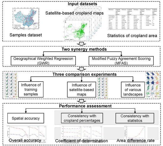
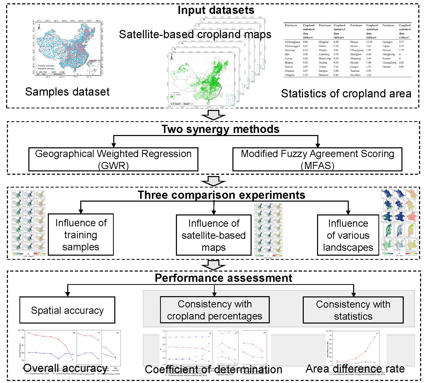
3. Data and Experiment Design

We designed three comparison experiments using various sets of training samples, multiple cropland maps with different accuracy, and different landscapes (Figure 1). We chose China as our study area (Figure 2). A total of seven satellite-based cropland maps at varying spatial resolution were used in this study. The results of experiments were assessed and compared by spatial accuracy, consistency with cropland percentage of validation samples, and consistency with cropland area from the agricultural statistics.

3.1. Data and processing

Seven satellite-based cropland maps, including GlobeLand30, Climate Change Initiative land cover product (CCI-LC), MODIS Collection5, MODIS Cropland, GlobCover 2009, Unified Cropland, and the National land use/cover database of China (NLUD-C) 2010 were used for synergy cropland mapping of China in 2010. The GlobeLand30 map is at 30 m spatial resolution and was produced based on Landsat and HJ-1 satellite images using a pixel-object-knowledge method [30]. The CCI-LC map is a 300 m global land cover dataset based on the Medium Resolution Imaging Spectrometer Instrument (MERIS) time series data from 2008 to 2012 [31]. The MODIS Collection 5 land cover map was generated at 500 m spatial resolution based on MODIS bands 1–7 and the enhanced vegetation index (EVI) using a decision tree classification algorithm [9]. The MODIS Cropland map was developed from multiyear MODIS data with 250 m spatial resolution and cropland area statistics using a decision tree classification algorithm [10]. The GlobCover 2009 map is at 300 m spatial resolution and was produced by European Space Agency and the Université catholique de Louvain using time series of MERIS Fine Resolution 2009 mosaics [32]. The 2014 Unified Cropland Layer is at 250 m spatial resolution and was produced by combining the fittest products according to four dimensions: timeliness, legend, resolution, and confidence [33]. The NLUD-C map was produced from Landsat TM/ETM+ images by Chinese Academy of Sciences using human-machine interactive interpretation [34,35].

These cropland maps are based on different map projections, classification schemes, and spatial resolution. The preprocessing of these maps prior to the synergy mapping included projection transformation, cropland definition harmonization, and spatial resolution standardization. These input maps were first projected into the same map projection. We then harmonized the cropland definitions using the Food and Agriculture Organization (FAO) cropland definition as the common definition for the seven maps. The FAO cropland definition includes arable land and permanent crops. Pure cropland and mosaic cropland classes were given high and low weights, respectively [5]. Table S2 from the online Supplementary Material shows the cropland definitions and modified cropland percentage of the input maps. Finally, all maps were resampled to 500 m spatial resolution with the average cropland percentage.

A total of 2800 cropland samples and 2851 noncropland samples were used for the experiments. Among them, 443 cropland samples and 1687 noncropland samples were obtained from Tsinghua University (http://data.ess.tsinghua.edu.cn/). In the collection scheme of samples from Tsinghua University, the entire globe was partitioned by about 7000 equal area hexagons using DGGRID software, and 10 samples were selected randomly in each hexagon [36]. The land cover types were identified by visual interpretation via high resolution images. As there are only 443 cropland samples in China which is not enough for experiments, the other samples were collected from the study of Lu et al. (2017). In the sampling frame of Lu et al. (2017), the samples were selected by using the stratified random sampling method based on the agreement of input cropland maps [5], and their land cover types were identified by Google Earth images (provided by DigitalGlobe’s WorldView-2 satellite sensor and obtained from the Google Earth Pro software) circa 2010. For each of these samples (pixels) that were identified, we estimated the cropland percentage within the 500 m × 500 m pixel using Google Earth images. In this study, we used a stratified random sampling method to divide training samples and validation samples. 70% of the total samples were selected randomly for training, and the rest (847 cropland samples, 848 noncropland samples) were used for validation (Figure S1 from the online Supplementary Material).

The statistics of cropland area in 2010 were acquired from the project of Second National Land Survey, the official national statistics in China. The cropland area was estimated based on survey base maps which were created by remote sensing images, and the definition of cropland was similar to that used by the FAO. In this research, the cropland area statistics at the province level (Table S3 from the online Supplementary Material) were used for calibration in the MFAS method.

3.2. Experiment Description

The accuracy of the seven harmonized cropland maps were assessed using the validation samples (

Table 1. Accuracy and consistency with cropland percentages and statistics of the seven harmonized cropland maps.

Cropland Maps	Overall Accuracy (%)	R2 between Maps and the Cropland Percentage	R2 between Maps and the Cropland Area Statistics
Unified Cropland	81.18	0.68	0.79
GlobeLand30	77.76	0.60	0.80
NLUD-C	76.76	0.55	0.83
MODIS Collection5	76.58	0.38	0.74
CCI-LC	75.69	0.36	0.58
MODIS Cropland	71.86	0.27	0.44
GlobCover 2009	69.50	0.23	0.38

). The maps with accuracy from high to low are Unified Cropland (#1), GlobeLand30 (#2), NLUD-C (#3), MODIS Collection 5 (#4), CCI-LC (#5), MODIS Cropland (#6), and GlobCover2009 (#7).

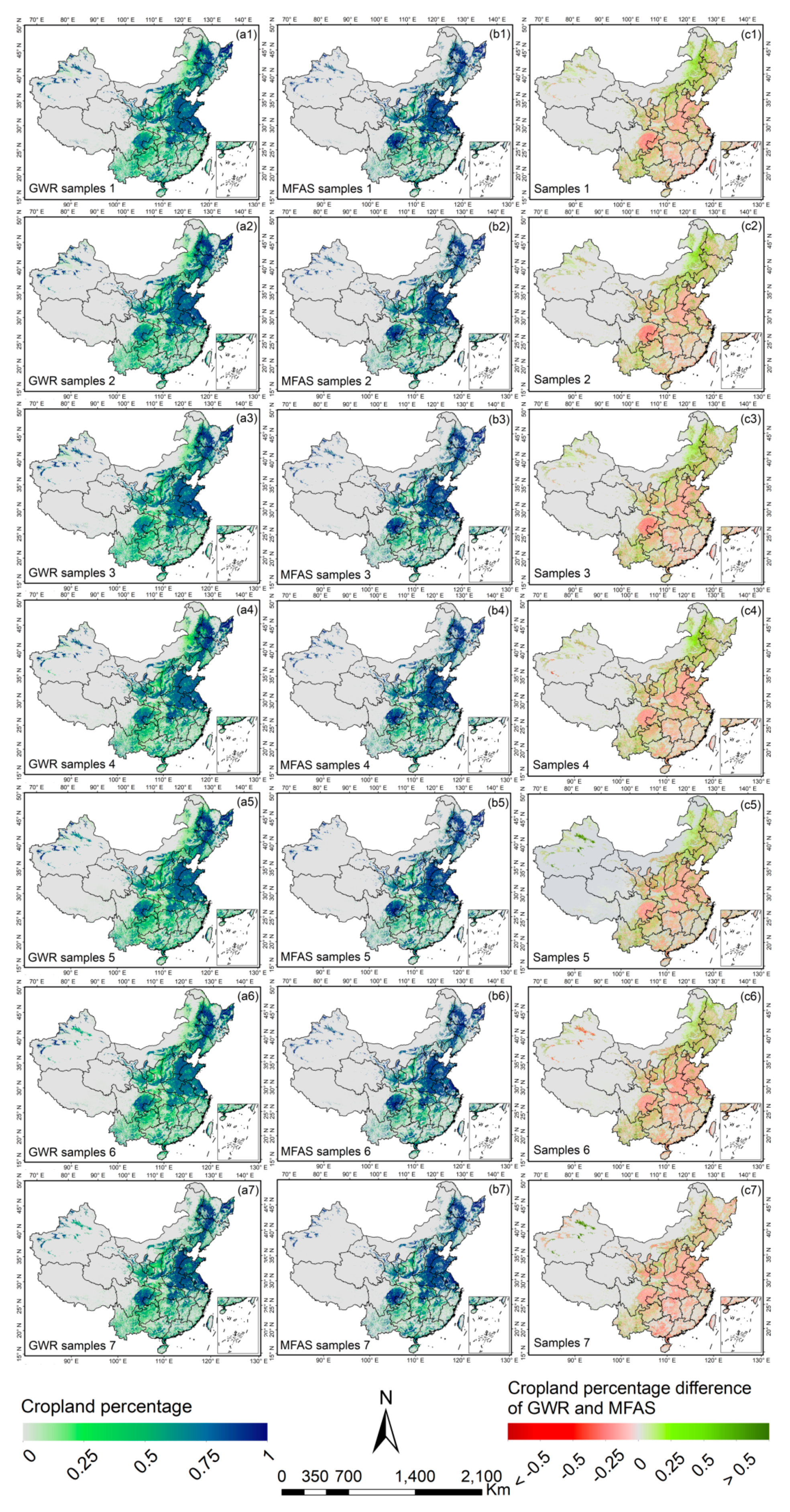
3.2.1. Synergy Cropland Mapping with Various Training Sample Sizes

In this experiment, we analyzed the influence of the size of training samples on the two synergy methods. Seven groups of training samples, including 90%, 70%, 50%, 30%, 10%, 5%, and 1% of the total training samples were randomly selected (

Table 2. The design of the experiment for assessing the influence of the size of training samples for synergy cropland mapping. The cropland maps used are Unified Cropland (#1), GlobeLand30 (#2), and NLUD-C (#3).

	Samples 1	Samples 2	Samples 3	Samples 4	Samples 5	Samples 6	Samples 7
Proportion of total training sample	90%	70%	50%	30%	10%	5%	1%
Cropland training samples	1777	1383	969	574	176	92	15
Noncropland training samples	1783	1386	1009	613	220	106	25
Validation samples	Cropland: 847 Noncropland: 848
Input datasets combination	#1, #2, #3

). In order to achieve best results, we chose the input map combination with the highest average accuracy (Unified Cropland, GlobeLand30, and NLUD-C) for synergy cropland mapping. The resulting maps were then used to evaluate the effects of the training sample size.

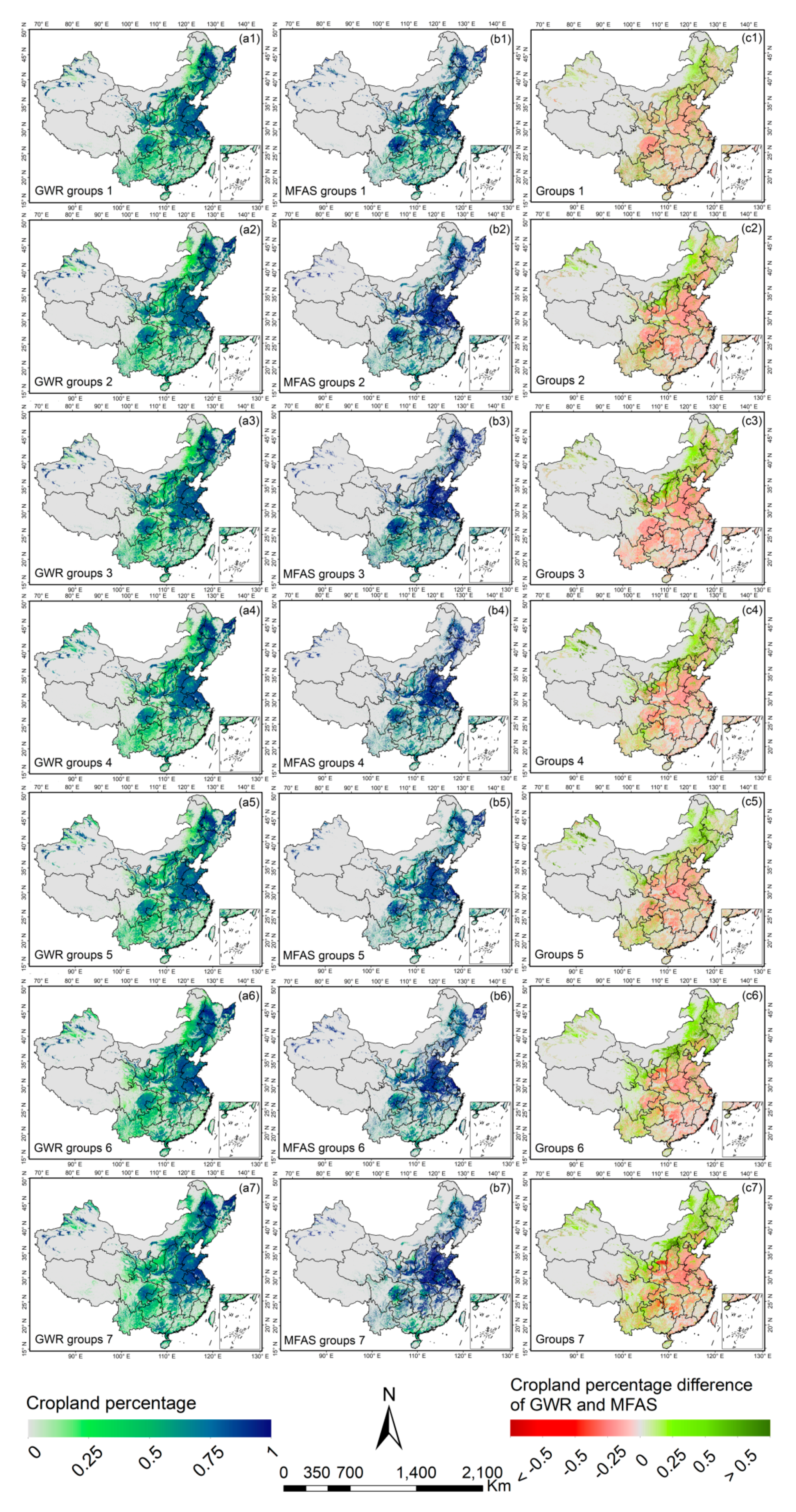
3.2.2. Synergy Cropland Mapping with Different Satellite-Based Maps

In this experiment, we assessed the influence of the quality of the input satellite-based map on the two synergy methods. All the training samples were employed for GWR and MFAS. We calculated the average accuracy of each combination of three input maps, and then selected seven groups of input map combinations, with their average accuracy ranging from high to low (

Table 3. The experiment design of the influence of input satellite-based map quality. The cropland maps used are Unified Cropland (#1), GlobeLand30 (#2), NLUD-C (#3), MODIS Collection 5 (#4), CCI-LC (#5), MODIS Cropland (#6), and GlobCover2009 (#7).

	Group 1	Group 2	Group 3	Group 4	Group 5	Group 6	Group 7
Input map combination	#1, #2, #3	#1, #4, #5	#1, #4, #6	#2, #5, #6	#2, #3, #7	#3, #5, #7	#5, #6, #7
Average accuracy (%)	78.57	77.82	76.54	75.10	74.67	73.98	72.35
Training samples	Cropland: 1953 Noncropland: 2003 Total: 3956
Validation samples	Cropland: 847   Noncropland: 848

). The combination of Unified Cropland, GlobeLand30, and NLUD-C had the highest overall accuracy (78.57%), followed by the combination of Unified Cropland, MODIS Collection 5, and CCI-LC. The combination including CCI-LC, MODIS Cropland, and GlobCover2009 had the lowest accuracy (72.35%). The synergy maps resulting from these experiments were then used to compare and analyze the effects of input satellite-based maps on synergy cropland mapping.

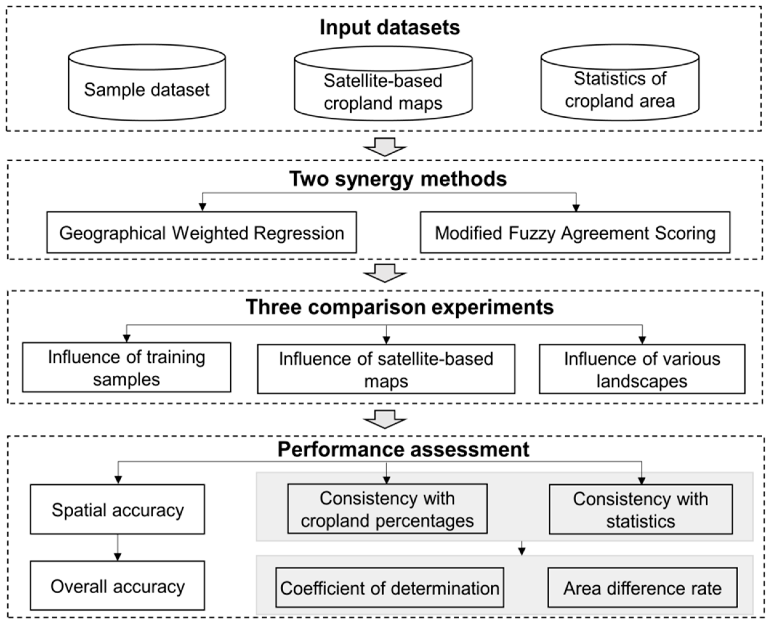
3.2.3. Synergy Cropland Mapping with Various Landscapes

In this experiment, we analyzed the influence of various landscapes on the two synergy methods. A series of studies showed that landscapes have distinct impacts on land cover/cropland mapping [12,13,37]. In China, the mountainous areas are usually characterized by heterogeneous landscapes, while plain areas generally represent homogeneous landscapes. Therefore, we used the elevation as an indicator to select areas with various landscapes for the comparison between GWR and MFAS. Chai et al. [38] divided the geomorphologic forms into plain (<20 m), hill (20–200 m), low mountain (200–500 m), medium mountain (500–1500 m), and high mountain (>1500 m). According to this standard, we chose five provinces including Jiangsu, Anhui, Henan, Shanxi, and Yunnan (Figure 2) for which mean elevations are shown in

Table 4. The experiment design of the influence of various landscapes.

		Test 1	Test 2	Test 3	Test 4	Test 5
Province		Jiangsu	Anhui	Henan	Shanxi	Yunnan
Landscape		Plain	Hill	Low mountain	Medium mountain	High mountain
Average DEM (m)		13.26	119.01	247.59	1160.68	1889.64
Validation samples	Cropland	74	70	70	60	35
	Noncropland	26	30	30	40	65

. All the training samples and input datasets were employed for the synergy mapping based on both GWR and MFAS. Then, results of the five provinces were extracted and assessed by 100 validation samples in each region.

3.3. Performance Assessment

The performance assessment included overall accuracy (OA), coefficient of determination (R²), and area difference rate (ADR), which were mainly calculated in ENVI software and IDL (Interactive Data Language). The overall accuracy (OA) was used to assess the accuracy of the synergy results. The overall accuracy is calculated as follows:

$$OA=\frac{n_c}{n}\times 100\%$$

(4)

where $n_c$ is the number of pixels that were correctly classified, and $n$ is the total number of pixels. According to Pontius and Millones (2010), we did not choose the Kappa coefficient to assess accuracy because it was misleading or flawed for practical applications [39].

The coefficient of determination (R²) was used to evaluate the correlation between the fusion cropland percentage and the cropland percentage identified from high-resolution images (i.e., the cropland percentage from the Google Earth), and the correlation between the fusion provincial cropland area and the cropland area statistical data. The area difference rate (ADR) was used to assess the degree of difference between a single fusion cropland area and a real cropland area. ADR is calculated as follows:

$$ADR=\frac{\left|c_p-s_p\right|}{s_p}\times 100\%$$

(5)

where $c_p$ is the cropland area of a single province $p$ estimated by the synergy map and $s_p$ is the cropland area statistical data of the province $p$ as the reference.

4. Results

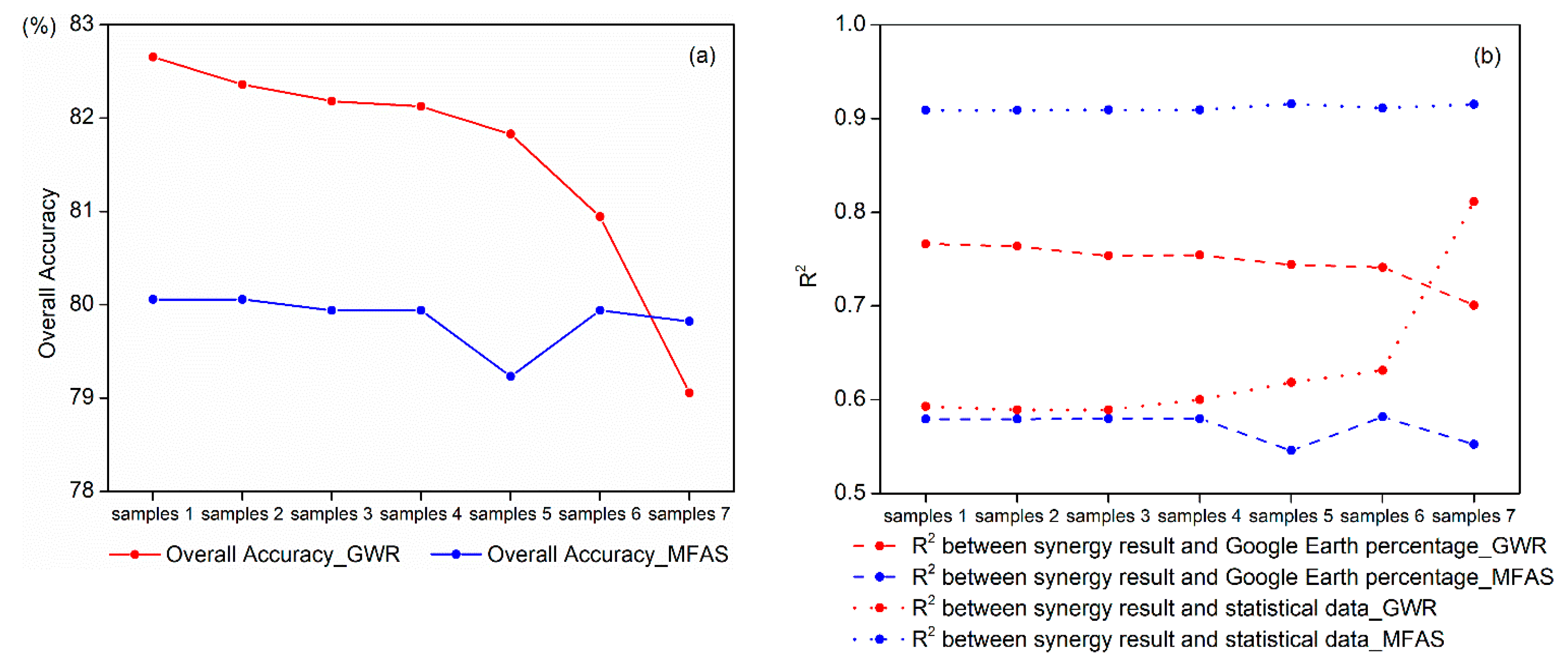
4.1. Influence of Training Samples

The two synergy methods (GWR and MFAS) were employed for cropland mapping with multiple sets of training samples (Table 2). The two methods led to similar cropland distributions but exhibited large differences in cropland percentage (Figure 3). The cropland percentage predicted by MFAS was higher than that by GWR in some regions such as Sichuan Basin, Hunan Province, and North China Plain. This pattern was more obvious when the number of training samples decreased. By contrast, the cropland percentage predicted by GWR was higher than that by MFAS in Inner Mongolia and Xinjiang.

We compared spatial accuracy, consistency with the cropland percentage identified from high-resolution images, and consistency with the statistics to assess how the performances of GWR and MFAS varied with the size of training samples (Figure 4). The overall accuracy of the GWR synergy results slightly decreased with the reduction in the number of training samples, particularly when the number of training samples was less than 10% of the original samples. The training sample size had no significant effects on the overall accuracy of MFAS synergy results (Figure 4a). For the consistency with the cropland percentage identified from high-resolution images, when the training samples decreased, there was a slight reduction in R² between the GWR synergy results and the cropland percentage identified from high-resolution images. The impact of training samples on the R² between the MFAS synergy results and the cropland percentage identified from high-resolution images was small. For the consistency with cropland area statistics, as the training samples decreased, the R² between the GWR synergy results and the cropland area statistical data gradually increased. The R² values between the MFAS synergy results and cropland area statistical data were stable and higher than those of the GWR synergy results (Figure 4b).

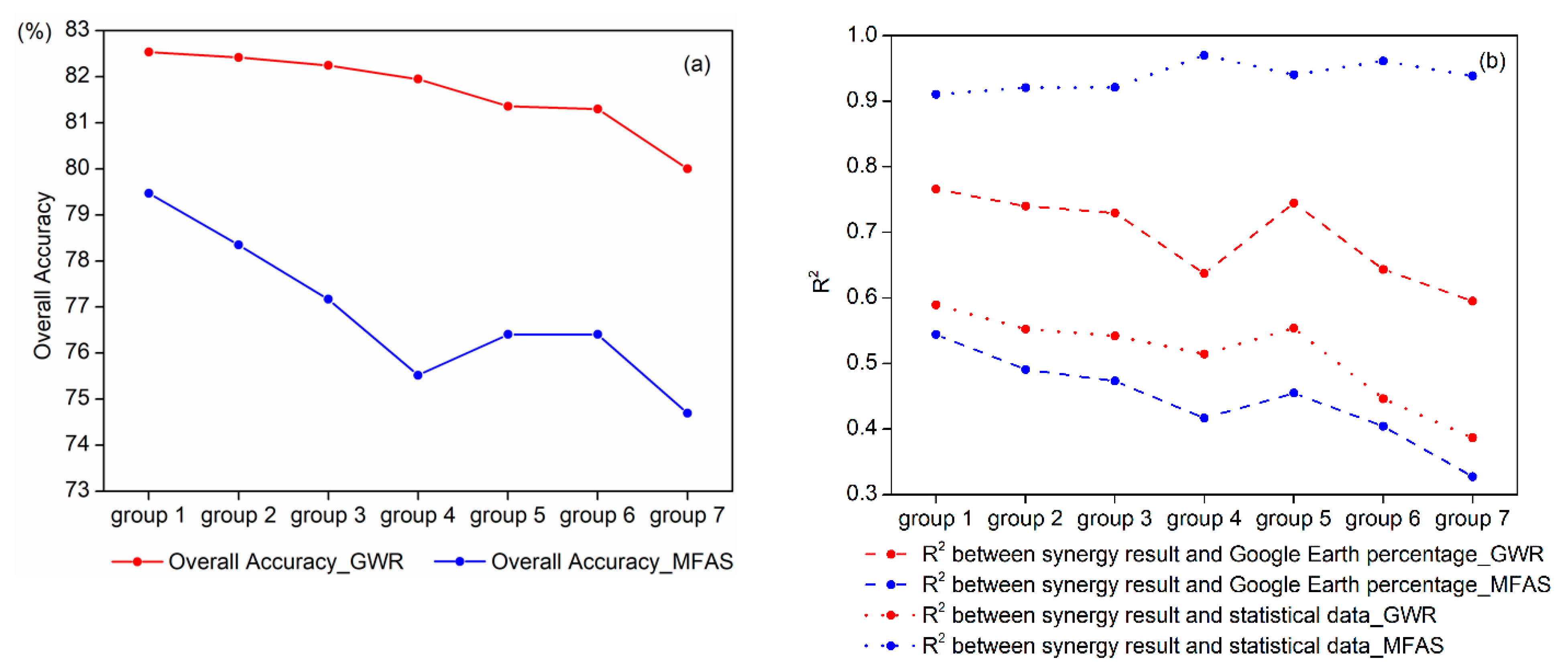
4.2. Influence of Satellite-Based Maps

We selected three of the seven maps to form seven combinations with various average accuracy. These combinations of satellite-based maps were applied for GWR and MFAS to generate synergy cropland maps (Figure 5). With the decrease in the average accuracy of the input maps, the difference in the cropland percentage predicted using the two methods increased, particularly in Shaanxi Province and near the border of Shanxi and Inner Mongolia Provinces (Figure 5c1–c7). When the average accuracy of the input maps was the lowest, the difference between the two methods was the largest.

It is clear that the overall accuracy of the two synergy results decreased as the average accuracy of the input map combination decreased, and MFAS was more sensitive to the quality of input maps compared with GWR (Figure 6a). The R² values between both synergy methods and the cropland percentage identified from high-resolution images decreased with the reduction in the average accuracy of the input map combination. The average accuracy of the input map had significantly higher effects on the MFAS synergy results than on the GWR synergy results (Figure 6b). When the average accuracy of the dataset decreased, the R² between the GWR synergy results and cropland area statistical data gradually decreased. However, the R² between the MFAS synergy results and cropland area statistical data remained at high levels all the time and only slightly changed (Figure 6b).

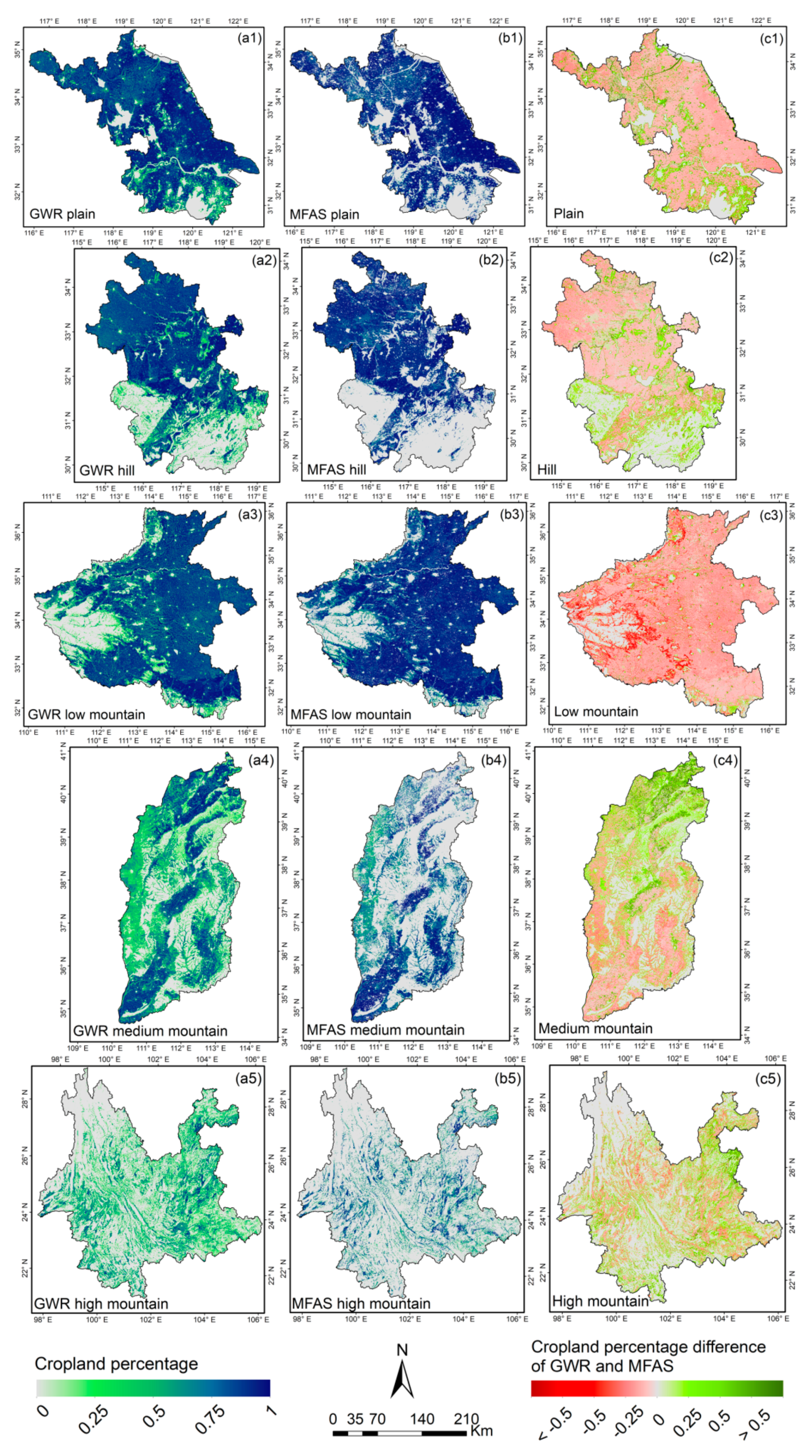
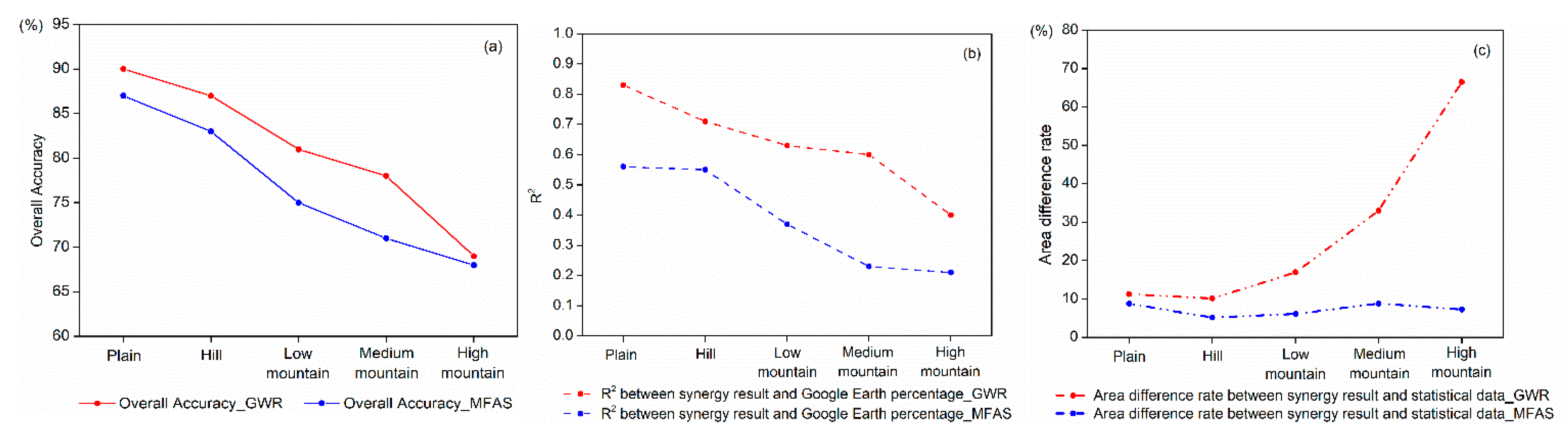
4.3. Influence of Various Landscapes

To evaluate the effects of different landscapes on the synergy mapping of the two methods, we selected five regions of different landscapes for comparative experiments. In plain, hill, and low mountain areas, the percentage of cropland predicted by MFAS was slightly higher than that by GWR (Figure 7). In medium mountain and high mountain areas where the average elevation is above 500 m, the percentage of cropland predicted by GWR was gradually higher than that by MFAS.

This shows that with increases in average elevation, the overall accuracy of the GWR synergy maps decreased (Figure 8a). At elevations higher than 1500 m, the overall accuracy of GWR sharply decreased. The overall accuracy of the MFAS also decreased with the increase in average elevation. When the elevation is higher than 200 m, the overall accuracy of MFAS synergy maps dramatically decreased. The variation trends in R² between both synergy results and the cropland percentage identified from high-resolution images (Figure 8b) were consistent with the overall accuracy trends (Figure 8a). The area difference rate between the cropland area of the GWR synergy results and cropland area statistical data was higher than that between the cropland area of the MFAS synergy results and cropland area statistical data. As the average elevation increased, the gap between the area difference rates of two approaches also gradually increased. Particularly for the GWR model, when the elevation is higher than 500 m, the area difference rate obviously increased (Figure 8c). However, the effect of various landscapes on the area difference rates between the cropland area of the MFAS synergy results and cropland area statistical data was relatively low and not obvious.

5. Discussion

The GWR model is a regression analysis based on the cropland percentage of the training samples [18,40], while the MFAS method mainly depends on the consistency of input datasets, and the training samples only play an auxiliary role [29]. We conducted three experiments to analyze the influence of the size of training samples, the quality of satellite-based cropland maps, and changes in landscapes on the performance of the two methods. GWR generally has higher overall accuracy and better consistency of cropland percentage, while MFAS has better consistency with cropland area statistics.

Training samples are essential input data for the synergy methods. GWR is more sensitive to and dependent on training samples than MFAS. For GWR, the more training samples, the more accurate the synergy map is and the closer the predicted value is to the real value. Previous studies showed that the representativeness in quality and quantity of training samples, as well as their spatial homogeneity, were quite important for the GWR model [20,41,42]. We also found that when the samples were relatively sufficient, the overall accuracy of the GWR synergy maps was slightly higher than that of the MFAS synergy maps. However, when the number of training samples was very small, the overall accuracy of the GWR synergy maps was lower than that of MFAS. With the number of training samples decreasing, the overall accuracy of the GWR maps and the MFAS maps decreased by 3.60% and 1.36%, respectively. GWR was slightly more sensitive to changes in the number of training samples than MFAS.

The quality of input maps has a significant impact on both methods, particularly on MFAS. The MFAS method is based on the data consistency [4,29]. Previous studies have shown that the quality of the input maps is important for synergy methods based on data consistency [5,29,43]. The improvement in the quality of input datasets can improve the accuracy of the resulting synergy maps [29]. Similarly, we found that the quality of the input maps influenced the accuracy of the MFAS synergy maps (Figure 5). Our results indicated that as the quality of the input maps decreased, the overall accuracy of the MFAS and GWR synergy maps decreased by 4.78% and 2.53%, respectively. The GWR method was less affected because the cropland percentage of the training samples was directly used.

The landscape is another important factor influencing the performance of the two synergy methods. Our results showed that the accuracy of the MFAS synergy maps was significantly affected by landscapes when the elevation is higher than 200 m. The GWR synergy maps were significantly affected only when the elevation is above 1500 m. The quality of the training samples and input maps was related to the landscape pattern. In heterogeneous regions with high elevation, the croplands are generally fragmented, and the consistency of the input satellite-based maps is typically lower [13]. Our results showed that MFAS was more sensitive to the changes in landscape. In the absence of higher resolution and more accurate input cropland maps, GWR was better than MFAS for heterogeneous areas. Lesiv et al. [25] also indicated that, in global forest mapping, GWR was more suited to regions with highly fragmented landscapes than other methods.

Compared to the GWR model, the MFAS method can generate synergy maps with a higher correlation with the cropland statistics. That is because MFAS uses the statistics data to calibrate the initial synergy maps, while the GWR model only considers the spatial distribution of cropland and does not involve the distribution of cropland areas. Schepaschenko et al. [20] compared a “best guess” hybrid global forest map by GWR and a hybrid global forest map calibrated with FAO FRA (Forest Resource Assessment) statistics. Their research showed that at the national scale, there were some differences between forest area based on GWR and forest area calibrated by FAO statistics partly because FAO FRA considers forest as land use rather than land cover [20]. Similarly, GWR considers cropland as land cover, while MFAS considers cropland as land use. It should be noted that when the number of the training samples decreased, the correlation between the GWR synergy maps and the cropland statistics increased. The reason is that the three input datasets used for synergy are highly correlated with statistical data. When the number of training samples decreased, the influence of input maps on the fusion results became larger, the prediction results were closer to the input maps which were used for regression, and the correlation between the GWR synergy result and the statistical data increased.

Cropland percentage predicted by the GWR has higher consistency with the cropland percentage identified from high-resolution image, compared with MFAS. GWR uses cropland percentage samples for regression, while MFAS employs the agreement of input maps to conduct experiments. In the MFAS method, the samples are only used to assess the overall accuracy of the input maps and to establish a detailed scoring table. However, GWR generally overestimated cropland percentage, such as some areas in the south and northwest of China. In these areas, the cropland is relatively fragmented and scarce [44]. Meanwhile, in the GWR model, regression parameters depend on geographical locations [28], and those pixels closer to croplands are more likely to be predicted as cropland areas. Many rivers and lakes are usually surrounded by croplands because of sufficient water supply for irrigation. The cropland percentage of those pixels at the junction of croplands and rivers/lakes was overestimated.

Method selection is dependent on the input data, landscape, and application purpose. The input data is the vital baseline information for synergy mapping. Because GWR is more dependent on training samples, when training samples are insufficient, MFAS is a better choice. For homogeneous regions, the input cropland products usually have higher accuracies and better consistencies. Therefore, MFAS is also a good alternative because of its easier and faster operation. For heterogeneous regions, GWR is a better choice because it outperforms other methods [25]. MFAS can generate a synergy map which has higher correlation with cropland statistics; therefore, this method is recommended for synergy map applications that require accuracy cropland area, such as yield estimation [45] and crop distribution mapping [46]. Meanwhile, for some applications, such as cropland fragmentation analysis [47], GWR is suitable to generate synergy maps because of its accurate cropland percentage. In this study, we only compared the two synergy methods GWR and MFAS. In the future, we will make more comparison experiments, including Naive Bayes and Logistic Regression among others, to provide more references for method selection.

6. Conclusions

Identifying the advantages and limitations of different synergy methods is critical for generating accurate spatial distribution information for synergy cropland mapping. In this study, we assessed and compared the influences of the size of training samples, quality of satellite-based cropland maps, and changes in landscapes on the performance of two synergy methods: MFAS and GWR. We also analyzed the advantages, disadvantages, and regional adaptabilities of regression analysis methods and data consistency scoring methods. When the number of training samples was relatively large, the GWR method had a higher overall accuracy than the MFAS method. The MFAS method was less dependent on the samples, and thus it is more suitable where the number of samples is relatively small. The quality of the satellite-based maps influenced both methods, particularly MFAS. Furthermore, GWR was less sensitive to changes in landscapes than MFAS. Cropland areas estimated by MFAS were more correlated with cropland area statistical data, while the cropland percentage predicted by GWR was closer to the values as identified from high-resolution images in magnitude. The GWR model is more suitable for regions with heterogeneous landscapes such as hills and low mountain areas, but the premise is that the cropland is more widely distributed. On the contrary, MFAS is more suitable for regions with homogeneous landscapes such as plain areas. MFAS is adequate for producing a global or regional large-scale cropland map that can be used in a global economic, biophysical, and other land use model, because it deals with cropland maps as land use types. If the GWR maps are applied for land use models, calibration by statistical data (such as FAO) is necessary. MFAS is more economical than GWR, because it is less dependent on sample data and computing resources.

References

1. Foley, J.A.; Ramankutty, N.; Brauman, K.A.; Cassidy, E.S.; Gerber, J.S.; Johnston, M.; Mueller, N.D.; O’Connell, C.; Ray, D.K.; West, P.C.; et al. Solutions for a cultivated planet. Nature 2011, 478, 337–342. [Google Scholar] [CrossRef] [PubMed] [Green Version]
2. Kearney, J. Food consumption trends and drivers. Philos. Trans. R. Soc. B 2010, 365, 2793–2807. [Google Scholar] [CrossRef] [PubMed] [Green Version]
3. Godfray, H.; Beddington, J.; Crute, I.; Haddad, L.; Lawrence, D.; Muir, J.; Pretty, J.; Robinson, S.; Thomas, S.; Toulmin, C. Food security: The challenge of feeding 9 billion people. Science 2010, 327, 812–818. [Google Scholar] [CrossRef] [PubMed]
4. Fritz, S.; See, L.; Mccallum, I.; You, L.; Bun, A.; Moltchanova, E.; Duerauer, M.; Albrecht, F.; Schill, C.; Perger, C.; et al. Mapping global cropland and field size. Glob. Chang. Biol. 2015, 21, 1980–1992. [Google Scholar] [CrossRef] [Green Version]
5. Lu, M.; Wu, W.; You, L.; Chen, D.; Zhang, L.; Yang, P.; Tang, H. A synergy cropland of china by fusing multiple existing maps and statistics. Sensors 2017, 17, 1613. [Google Scholar] [CrossRef] [PubMed]
6. Stansfield, J. The United Nations sustainable development goals (SDGs): A framework for intersectoral collaboration. Whanake Pac. J. Community Dev. 2017, 3, 38–49. [Google Scholar]
7. Bartholome, E.; Belward, A.S. GLC2000: A new approach to global land cover mapping from earth observation data. Int. J. Remote Sens. 2005, 26, 1959–1977. [Google Scholar] [CrossRef]
8. Hansen, M.; Defries, R.; Townshend, J.; Sohlberg, R. Global land cover classification at 1 km spatial resolution using a classification tree approach. Int. J. Remote Sens. 2000, 21, 1331–1364. [Google Scholar] [CrossRef] [Green Version]
9. Friedl, M.; Sulla-Menashe, D.; Tan, B.; Schneider, A.; Ramankutty, N.; Sibley, A.; Huang, X. MODIS collection 5 global land cover: Algorithm refinements and characterization of new datasets. Remote Sens. Environ. 2010, 114, 168–182. [Google Scholar] [CrossRef]
10. Pittman, K.; Hansen, M.; Beckerreshef, I.; Potapov, P.; Justice, C. Estimating global cropland extent with multi-year MODIS data. Remote Sens. 2010, 2, 1844–1863. [Google Scholar] [CrossRef]
11. Chen, J.; Chen, J.; Liao, A.; Cao, X.; Chen, L.; Chen, X.; Peng, S.; Han, G.; Zhang, H.; He, C.; et al. Concepts and key techniques for 30 m global land cover mapping. Acta Geod. Cartogr. Sinica 2014, 43, 551–557. (In Chinese) [Google Scholar]
12. Wu, W.; Shibasaki, R.; Yang, P.; Zhou, Q.; Tang, H. Remotely sensed estimation of cropland in China: A comparison of the maps derived from four global land cover datasets. Can. J. Remote Sens. 2008, 34, 467–479. [Google Scholar] [CrossRef]
13. Lu, M.; Wu, W.; Zhang, L.; Liao, A.; Peng, S.; Tang, H. A comparative analysis of five global cropland datasets in China. Sci. China Earth Sci. 2016, 59, 2307–2317. [Google Scholar] [CrossRef]
14. Congalton, R.; Gu, J.; Yadav, K.; Ozdogan, M. Global land cover mapping: A review and uncertainty analysis. Remote Sens. 2014, 6, 12070–12093. [Google Scholar] [CrossRef]
15. Yu, L.; Wang, J.; Clinton, N.; Xin, Q.; Zhong, L.; Chen, Y.; Gong, P. FROM-GC: 30 m global cropland extent derived through multisource data integration. Int. J. Digit. Earth 2013, 6, 521–533. [Google Scholar] [CrossRef]
16. Liang, L.; Gong, P. Evaluation of global land cover maps for cropland area estimation in the conterminous United States. Int. J. Digit. Earth 2015, 8, 102–117. [Google Scholar] [CrossRef]
17. Castanedo, F. A review of data fusion techniques. Sci. World J. 2013, 2013, 704504. [Google Scholar] [CrossRef]
18. See, L.; Schepaschenko, D.; Lesiv, M.; McCallum, I.; Fritz, S.; Comber, A.; Perger, C.; Schill, C.; Zhao, Y.; Maus, V.; et al. Building a hybrid land cover map with crowdsourcing and geographically weighted regression. ISPRS J. Photogramm. Remote Sens. 2015, 103, 48–56. [Google Scholar] [CrossRef] [Green Version]
19. Verburg, P.; Neumann, K.; Nol, L. Challenges in using land use and land cover data for global change studies. Glob. Chang. Biol. 2011, 17, 974–989. [Google Scholar] [CrossRef] [Green Version]
20. Schepaschenko, D.; See, L.; Lesiv, M.; Mccallum, I.; Fritz, S.; Salk, C.; Moltchanova, E.; Perger, C.; Shchepashchenko, M.; Shvidenko, A.; et al. Development of a global hybrid forest mask through the synergy of remote sensing, crowdsourcing and FAO statistics. Remote Sens. Environ. 2015, 162, 208–220. [Google Scholar] [CrossRef]
21. Chen, D.; WU, W.; Lu, M.; Hu, Q.; Zhou, Q. Progresses in land cover data reconstruction method based on multi-source data fusion. Chin. J. Agric. Resour. Reg. Plan. 2016, 37, 62–70. (In Chinese) [Google Scholar]
22. Kinoshita, T.; Iwao, K.; Yamagata, Y. Creation of a global land cover and a probability map through a new map integration method. Int. J. Appl. Earth Obs. Geoinf. 2014, 28, 70–77. [Google Scholar] [CrossRef]
23. Jung, M.; Henkel, K.; Herold, M.; Churkina, G. Exploiting synergies of global land cover products for carbon cycle modeling. Remote Sens. Environ. 2006, 101, 534–553. [Google Scholar] [CrossRef]
24. Clinton, N.; Yu, L.; Gong, P. Geographic stacking: Decision fusion to increase global land cover map accuracy. Glob. Land Cover Mapp. Monit. 2015, 103, 57–65. [Google Scholar] [CrossRef]
25. Lesiv, M.; Moltchanova, E.; Schepaschenko, D.; See, L.; Shvidenko, A.; Comber, A.; Fritz, S. Comparison of data fusion methods using crowdsourced data in creating a hybrid forest cover map. Remote Sens. 2016, 8, 261. [Google Scholar] [CrossRef]
26. Fritz, S.; McCallum, I.; Schill, C.; Perger, C.; Grillmayer, R.; Achard, F.; Kraxner, F.; Obersteiner, M. Geo-wiki.org: The use of crowdsourcing to improve global land cover. Remote Sens. 2009, 1, 345–354. [Google Scholar] [CrossRef]
27. Fritz, S.; McCallum, I.; Schill, C.; Perger, C.; See, L.; Schepaschenko, D.; van der Velde, M.; Kraxner, F.; Obersteiner, M. Geo-wiki: An online platform for improving global land cover. Environ. Model. Softw. 2012, 31, 110–123. [Google Scholar] [CrossRef]
28. Fotheringham, A.S.; Charlton, M.E.; Brunsdon, C. Geographically weighted regression: A natural evolution of the expansion method for spatial data analysis. Environ. Plan. A 1998, 30, 1905–1927. [Google Scholar] [CrossRef]
29. Fritz, S.; You, L.; Bun, A.; See, L.; Mccallum, I.; Schill, C.; Perger, C.; Liu, J.; Hansen, M.; Obersteiner, M. Cropland for sub-saharan Africa: A synergistic approach using five land cover data sets. Geophys. Res. Lett. 2011, 38, 155–170. [Google Scholar] [CrossRef]
30. Chen, J.; Chen, J.; Liao, A.; Cao, X.; Chen, L.; Chen, X.; He, C.; Han, G.; Peng, S.; Lu, M.; et al. Global land cover mapping at 30 m resolution: A POK-based operational approach. ISPRS J. Photogramm. Remote Sens. 2015, 103, 7–27. [Google Scholar] [CrossRef]
31. Defourny, P.; Kirches, G.; Brockmann, C.; Boettcher, M.; Peters, M.; Bontemps, S.; Lamarche, C.; Schlerf, M.; Santoro, M. Land Cover CCI: Product User Guide Version 2. Available online: http://maps.elie.ucl.ac.be/CCI/viewer/download/ESACCI-LC-PUG-v2.5.pdf (accessed on 8 February 2018).
32. Bontemps, S.; Defourny, P.; Bogaert, E.; Arino, O.; Kalogirou, V.; Perez, J. GLOBCOVER 2009. Products Description and Validation Report. Available online: https://core.ac.uk/download/pdf/11773712.pdf (accessed on 8 February 2018).
33. Waldner, F.; Fritz, S.; Di Gregorio, A.; Defourny, P. Mapping priorities to focus cropland mapping activities: Fitness assessment of existing global, regional and national cropland maps. Remote Sens. 2015, 7, 7959–7986. [Google Scholar] [CrossRef]
34. Zhang, Z.; Wang, X.; Zhao, X.; Liu, B.; Yi, L.; Zuo, L.; Wen, Q.; Liu, F.; Xu, J.; Hu, S. A 2010 update of National land use/cover database of China at 1: 100000 scale using medium spatial resolution satellite images. Remote Sens. Environ. 2014, 149, 142–154. [Google Scholar] [CrossRef]
35. Ning, J.; Liu, J.; Kuang, W.; Xu, X.; Zhang, S.; Yan, C.; Li, R.; Wu, S.; Hu, Y.; Du, G.; et al. Spatiotemporal patterns and characteristics of land-use change in China during 2010–2015. J. Geogr. Sci. 2018, 28, 547–562. [Google Scholar] [CrossRef]
36. Gong, P.; Wang, J.; Yu, L.; Zhao, Y.; Zhao, Y.; Liang, L.; Niu, Z.; Huang, X.; Fu, H.; Liu, S.; et al. Finer resolution observation and monitoring of GLC: First mapping results with Landsat TM and ETM+ data. Int. J. Remote Sens. 2013, 34, 2607–2654. [Google Scholar] [CrossRef]
37. Xiong, J.; Thenkabail, P.; Gumma, M.; Teluguntla, P.; Poehnelt, J.; Congalton, R.; Yadav, K.; Thau, D. Automated cropland mapping of continental Africa using Google Earth engine cloud computing. ISPRS. J. Photogramm. 2017, 126, 225–244. [Google Scholar] [CrossRef]
38. Chai, Z. The Suggestion of Using Relative Altitude to Divide the Geomorphologic Forms. In Geographical Society of China. Theses of Geomorphology; Science Press: Beijing, China, 1983; pp. 90–97. (In Chinese) [Google Scholar]
39. Pontius, R.G.; Millones, M. Death to Kappa: Birth of quantity disagreement and allocation disagreement for accuracy assessment. Int. J. Remote Sens. 2011, 32, 4407–4429. [Google Scholar] [CrossRef]
40. Schepaschenko, D.; Shvidenko, A.; Lesiv, M.; Ontikov, P.; Shchepashchenko, M.V.; Kraxner, F. Estimation of forest area and its dynamics in Russia based on synthesis of remote sensing products. Contemp. Probl. Ecol. 2015, 8, 811–817. [Google Scholar] [CrossRef] [Green Version]
41. Zhong, L.; Gong, P.; Biging, G.S. Efficient corn and soybean mapping with temporal extendability: A multi-year experiment using Landsat imagery. Remote Sens. Environ. 2014, 140, 1–13. [Google Scholar] [CrossRef]
42. Hu, Q.; Ma, Y.; Xu, B.; Song, Q.; Tang, H.; Wu, W. Estimating sub-pixel soybean fraction from time-series modis data using an optimized geographically weighted regression model. Remote Sens. 2018, 10, 491. [Google Scholar] [CrossRef]
43. Pérez-Hoyos, A.; García-Haro, F.; San-Miguel-Ayanz, J. A methodology to generate a synergetic land-cover map by fusion of different land-cover products. Int. J. Appl. Earth Obs. Geoinf. 2012, 19, 72–87. [Google Scholar] [CrossRef]
44. Chen, D.; Yu, Q.; Hu, Q.; Xiang, M.; Zhou, Q.; Wu, W. Cultivated land change in the Belt and Road Initiative region. J. Geogr. Sci. 2018, 28, 1580–1594. [Google Scholar] [CrossRef]
45. Monfreda, C.; Ramankutty, N.; Foley, J.A. Farming the planet: 2. Geographic distribution of crop areas, yields, physiological types, and net primary production in the year 2000. Global Biogeochem. Cycles 2008, 22, GB1022. [Google Scholar] [CrossRef]
46. You, L.; Wood, S.; Wood-Sichra, U.; Wu, W. Generating global crop distribution maps: From census to grid. Agr. Syst. 2014, 127, 53–60. [Google Scholar] [CrossRef] [Green Version]
47. Yu, Q.; Hu, Q.; Vliet, J.; Verburg, P.; Wu, W. GlobeLand30 shows little cropland area loss but greater fragmentation in China. Int. J. Appl. Earth. Obs. 2018, 66, 37–45. [Google Scholar] [CrossRef]
Figure 1. The flowchart of the comparison experiments.
Remotesensing 11 00213 g001
Figure 2. The study area: China and five provinces (Jiangsu, Anhui, Henan, Shanxi, Yunnan). The Digital Elevation Model (DEM) represents the landscapes of the study area. Synergy cropland mapping with various training sample sizes and synergy cropland mapping with different satellite-based maps were conducted in China. Synergy cropland mapping with various landscapes were conducted in five provinces.
Remotesensing 11 00213 g002
Figure 3. Synergy cropland results of: Geographically weighted regression (GWR) (left panel) and modified fuzzy agreement scoring (MFAS) (middle panel) and their difference images (right panel). Panels from top to bottom represent synergy results with various sample sets as shown in Table 2.
Remotesensing 11 00213 g003
Figure 4. Performance assessment and comparisons including spatial accuracy (a), consistency with cropland percentages, and consistency with cropland area from the statistics using various sample sets (b).
Remotesensing 11 00213 g004
Figure 5. Synergy cropland maps of GWR (left panel) and MFAS (middle panel) and their difference images (right panel). Panels from top to bottom represent synergy results with various average accuracy of input satellite-based map combinations as shown in Table 3.
Remotesensing 11 00213 g005
Figure 6. Performance assessment and comparisons including spatial accuracy (a), consistency with cropland percentage, and consistency with statistics using input satellite-based map combinations of various average accuracy (b).
Remotesensing 11 00213 g006
Figure 7. Synergy cropland maps of GWR (left panel) and MFAS (middle panel) and their difference images (right panel). Panels from top to bottom represent synergy results with various landscapes as shown in Table 4.
Remotesensing 11 00213 g007
Figure 8. Performance assessment and comparisons including spatial accuracy (a), consistency with cropland percentage (b), and consistency with statistics (c) using various landscapes.
Remotesensing 11 00213 g008