Article

Can We Use the QA4ECV Black-sky Fraction of Absorbed Photosynthetically Active Radiation (FAPAR) using AVHRR Surface Reflectance to Assess Terrestrial Global Change?

1
European Commission, Joint Research Centre, 21027 Ispra, Italy
2
NASA Goddard Space Flight Center, MD 20771, USA
*
Author to whom correspondence should be addressed.
Remote Sens. 2019, 11(24), 3055; https://doi.org/10.3390/rs11243055
Submission received: 16 October 2019 / Revised: 6 December 2019 / Accepted: 14 December 2019 / Published: 17 December 2019
(This article belongs to the Section Biogeosciences Remote Sensing)

Abstract

:
NOAA platforms provide the longest period of terrestrial observation since the 1980s. The progress in calibration, atmospheric corrections and physically based land retrieval offers the opportunity to reprocess these data for extending terrestrial product time series. Within the Quality Assurance for Essential Climate Variables (QA4ECV) project, the black-sky Joint Research Centre (JRC)-fraction of absorbed photosynthetically active radiation (FAPAR) algorithm was developed for the AVHRR sensors on-board NOAA-07 to -16 using the Land Surface Reflectance Climate Data Record. The retrieval algorithm was based on the radiative transfer theory, and uncertainties were included in the products. We proposed a time and spatial composite for providing both 10-day and monthly products at 0.05° × 0.05°. Quality control and validation were achieved through benchmarking against third-party products, including Sea-Viewing Wide Field-of-View Sensor (SeaWiFS) datasets produced with the same retrieval algorithm. Past ground-based measurements, providing a proxy of FAPAR, showed good agreement of seasonality values over short homogeneous canopies and mixed vegetation. The average difference between SeaWiFS and QA4ECV monthly products over 2002–2005 is about 0.075 with a standard deviation of 0.091. We proposed a monthly linear bias correction that reduced these statistics to 0.02 and 0.001. The complete harmonized long-term time series was then used to address its fitness for the purpose of analysis of global terrestrial change.

1. Introduction

The majority of solar radiation available to the Earth system is absorbed at or near the oceanic and continental surface. This energy is ultimately released to the atmosphere through fluxes of infrared radiation, as well as sensible and latent heat. The phytosphere, which itself accounts for most of biomass, affects these exchanges with the atmosphere through a contact surface (leaves) estimated to be larger than the surface of the entire planet [1]. The state and the evolution of terrestrial vegetation are characterized by a large number of physical, biochemical, and physiological variables. Few of these are directly observable from space, but they jointly determine the fraction of absorbed photosynthetically active radiation (FAPAR) that acts as an integrated indicator of the status and health of plant canopies and can be retrieved by space remote sensing techniques [2,3,4]. FAPAR plays a critical role in the global carbon cycle and in the determination of the primary productivity of the biosphere [5,6,7].
The properties of terrestrial surfaces thus concern a large number of users in such applications including agriculture, forestry, environmental monitoring, etc. [8,9,10]. Since plant canopies significantly affect the spectral and directional reflectance of solar radiation, the analysis of these reflectances leads to a better understanding of fundamental processes controlling the biosphere. This supports the policies of sustainable resources exploitation and the control of the effectiveness of any adopted rules and regulations. FAPAR is recognized as one of the terrestrial essential climate variables (ECVs) by the global climate observing system (GCOS) [11,12].
Three FAPAR products from Advanced Very-High-Resolution Radiometer (AVHRR) are currently available: the Global Inventory Modeling and Mapping Studies GIMMS3 products [13], NOAA’s National Centers for Environmental Information (NCEI) AVHRR FAPAR [14] and the Global LAnd Surface Satellite (GLASS) [15]. Xiao et al. (2018) [16] compared these three products and found that they are spatially consistent with a strong discrepancy over tropical forest regions at latitudes from 55°N to 65°N.
In the context of an FP-7 European project—Quality Assurance for Essential Climate Variables (QA4ECV), the Joint Research Centre (JRC)-FAPAR algorithm was designed for the AVHRR Land Surface Reflectance Climate Data Record v5.0 [17]. Further to the previously mentioned products, we generated three temporal scales (daily, 10-day, and monthly) at 0.05° × 0.05° with associated grid cell uncertainties. In addition, the 10-day and monthly data were regridded at 0.5° × 0.5°. Uncertainties were included in each processing step from error propagation to temporal and spatial composites. These various spatial and temporal datasets enabled validation of native products against ground-based measurements, and then how these datasets were used for global-scale analysis were explored. A generic system for implementation and evaluation of quality assurance (QA) was applied to provide traceability information [18]. In summary, the JRC-FAPAR retrieval method was used to assess the presence on the ground of live green vegetation. The main procedure provided an estimate of “green” FAPAR in the plant canopy. It is important to note that the retrieval value corresponds to the black-sky FAPAR at the time of data acquisition. Past JRC-FAPAR algorithms have been optimized for various optical instruments and operationally implemented with data from the Sea-Viewing Wide Field-of-View Sensor (SeaWiFS) [19], MEdium Resolution Imaging Spectrometer (MERIS) [20,21] and Copernicus Sentinel-3 Ocean and Land Colour Instrument (OLCI) [22]. Validation exercises at a medium spatial resolution have been performed for SeaWiFS [23,24], MERIS [24,25] and OLCI [26,27].
Recent studies of global terrestrial change, such as assessment of global “greenness”, exploited various Earth observation (EO) products [28]. At the same time, discussions on the fitness of several products for trend analysis showed that the results changed as a function of the products [29]. This means that, before any global analysis can be undertaken, both a validation process and a verification process are mandatory to assess, if a space product can be used to assess terrestrial global change. In addition, it is important to highlight that the uncertainty associated to the product should be available at each grid cell level. This information also helps to ingest these EO products into climate or land assimilation schemes.
In this paper, we therefore proposed to evaluate QA4ECV products against in situ and third-party data before using them for assessing terrestrial global change. We first presented the seasonal behaviour and magnitude of FAPAR against the in situ data, together with NCEI FAPAR products [14,30] and the JRC-Two-Stream Inversion Package (TIP) [31]. All the results were discussed, taking into account each respective FAPAR definition using outcomes from [32]. Secondly, we performed a more generic quality control over the QA4ECV virtual validation land sites defined in [33] from 1982 to 2006 using monthly products at 0.05° × 0.05°. The evaluation was then completed through direct comparisons against JRC-FAPAR daily global products from the SeaWiFS at 0.05° × 0.05° for the years 1999 and 2003 corresponding to the AVHRR2 and AVHRR3 satellites, respectively. A further comparison of the monthly products at 0.5° × 0.5° over 1998–2005 then allowed us to propose and apply a monthly-grid linear correction over the entire time series to harmonize all products from 1982 to 2006. We finally analyzed QA4ECV long time series and uncertainties in order to illustrate and discuss the global change of terrestrial surfaces. The paper was ended with a conclusion section.

2. Data Used

The AVHRR surface reflectance products [17,34] were used as inputs to derive the black-sky FAPAR. This dataset was produced using state-of-the-art algorithms for geolocation, calibration, cloud screening, and atmospheric and surface directional effect correction, to be able to achieve a data record as consistent as possible. The latter data were converted to bidirectional reflectance factors (BRFs) as done by [14] but using the native view zenith angles instead of the nadir view.
NCEI FAPAR daily products were used during comparison exercises against ground-based measurements. These were produced from an artificial neural network (ANN) calibrated using the Moderate Resolution Imaging Spectroradiometer (MODIS) FAPAR as training datasets [14]. This ANN was optimized over six land cover classes, but no retrieval was available over a bare or very sparsely vegetated area. The NCEI FAPAR refers to direct illumination, i.e., the black-sky FAPAR at local noon, which has the same leaf scattering albedo definition as that of the MODIS [14]. In addition, the JRC-TIP FAPAR was processed using the MODIS Collection 6 surface albedo and retrieved under the “green” foliage assumption. This permitted us to keep the assumption on the leaf scattering albedo used in the QA4ECV products. The JRC-TIP FAPAR was defined as the white-sky FAPAR, i.e., diffuse component. Because of these different definitions, we expected some bias as shown in [32].
The JRC products derived from the SeaWiFS were then used for a comparison of daily (0.05° × 0.05°) and monthly (0.5° × 0.5°) products at a global scale. These products were processed using the same retrieval algorithm with top-of-atmosphere (TOA) reflectances used as inputs [19].
Significant efforts were devoted in the past to the validation of surface products such as FAPAR [23,35,36,37]. However, ground-based FAPAR products suitable for validation can only be measured in fields with significant levels of difficulty. They are often a proxy of FAPAR, either derived from leaf area index (LAI) measurements or from the fraction of intercepted PAR (FIPAR). Impacts of different types of internal variability of an extinction coefficient (a rate of how the radiation is absorbed by a medium), together with the resolution of the sampled domain, were already analysed for clouds [38]. They established conditions, where three-dimensional (3D) effects can be anticipated to play a major role in the radiation transfer regime. Gobron et al. (2006) extrapolated their results to terrestrial land covers by associating the main radiative transfer regimes against statistical properties of the leaf extinction coefficient within the spatial domain of investigation [23]. In summary, the “fast” variability regime is associated with statistically homogeneous canopy, in which exists a Poisson distribution of the leaf density. The “slow” variability regime is associated with canopies, where the leaf angle distribution (LAD) is close enough to be locally homogeneous such that average local-scale flux values are representative. The last case, the “resonant” regime, is defined, where the spatial complexity is such that a typical photon beam samples various types of structures between entering and escaping the canopy.
Table 1 summarizes ground-based approaches to assessing insitu FAPAR values over different sites as done in [23], and Table 2 recapitulates the geolocations of field sites together with their transfer regimes and land cover types.

3. Methods

BRFs representing the AVHRR NOAA like surface data were created using the “semi-discrete” radiative transfer model [43] that represents the spectral and directional reflectances of horizontally homogeneous plant canopies and computes the values of the black-sky FAPAR. The sampling of vegetation parameters, such as LAI, height of canopies, leaf radius, soil albedo, and angular values, was chosen to cover a wide range of environmental and observation conditions. These simulations constituted the basic information used to optimize the algorithm for each AVHRR sensor on-board NOAA-07, -09, -11, and -14 platforms, taking into account their respective spectral responses. Once these simulated datasets were created, the design of the algorithm consisted in defining the mathematical combination of two spectral bands that best accounted for the variations of the variable of interest (in this case, it was the “green” black-sky FAPAR) on the basis of (simulated) measurements, while minimizing the effect of perturbing factors such as angular effects. The coefficients for each NOAA platform were detailed in [44].
The associated daily uncertainty, σ, was expressed as one standard deviation using the error propagation theory and derivatives. In order to compute daily σ, we set the surface reflectance uncertainties at 10%. In the temporal (spatial) composite method, additional uncertainties corresponded to the standard deviation of the FAPAR after removal of outliers. In the regridded products, the FAPAR at 0.5° × 0.5° corresponded to the weighted average of individual grid cell values, and the uncertainties were computed using the quadratic mean.
When performing, at the original resolution, the benchmark comparison of daily products, we first computed the accuracy (A) that statistically represented the mean bias between QA4ECV values and SeaWiFS products as proposed in [45]. We also provided the precision, P, which indicated the repeatability and was computed as the standard deviation of the estimates around the reference values corrected for the mean bias (accuracy). Finally, U was the actual statistical deviation of the estimates from the reference that included the mean bias [46]. The results were discussed in comparison to the QA4ECV FAPAR uncertainties, σ, as well as the spatial standard deviation, Sdev.
Next, a monthly linear correction was proposed to harmonize all the different NOAA products, as these suffered from calibration issues as shown in Section 4.5. This was done using the products over 2002–2005 by optimizing linear equations such as Equation (1):
Q m , x , y = a m S m , x , y + b m ,
where Q and S are the QA4ECV and SeaWiFS monthly products, respectively; m represents the month, and (x, y) is the coordinates of the grid cell at 0.5° × 0.5°; the coefficients a(m) and b(m) are optimized for each month using data from 2002 to 2005.

4. Benchmark Results

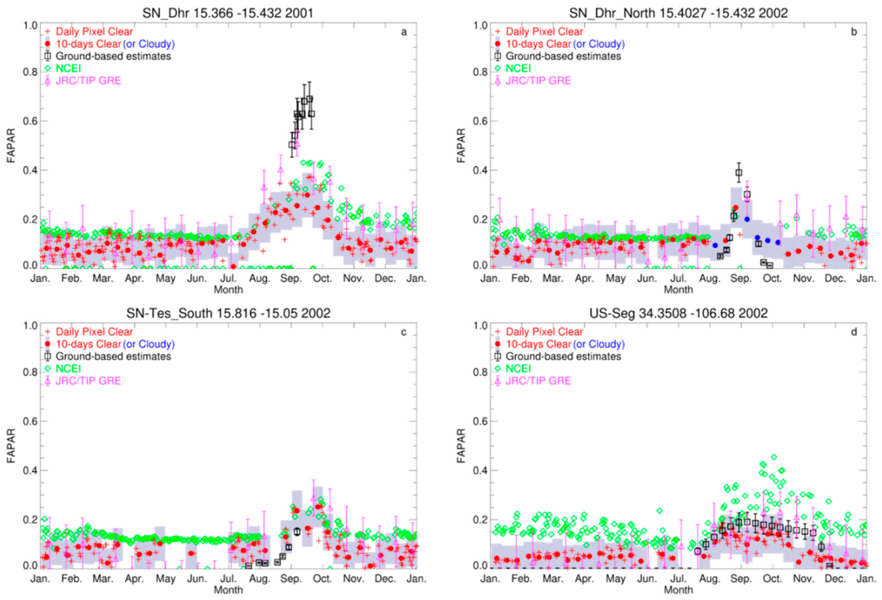
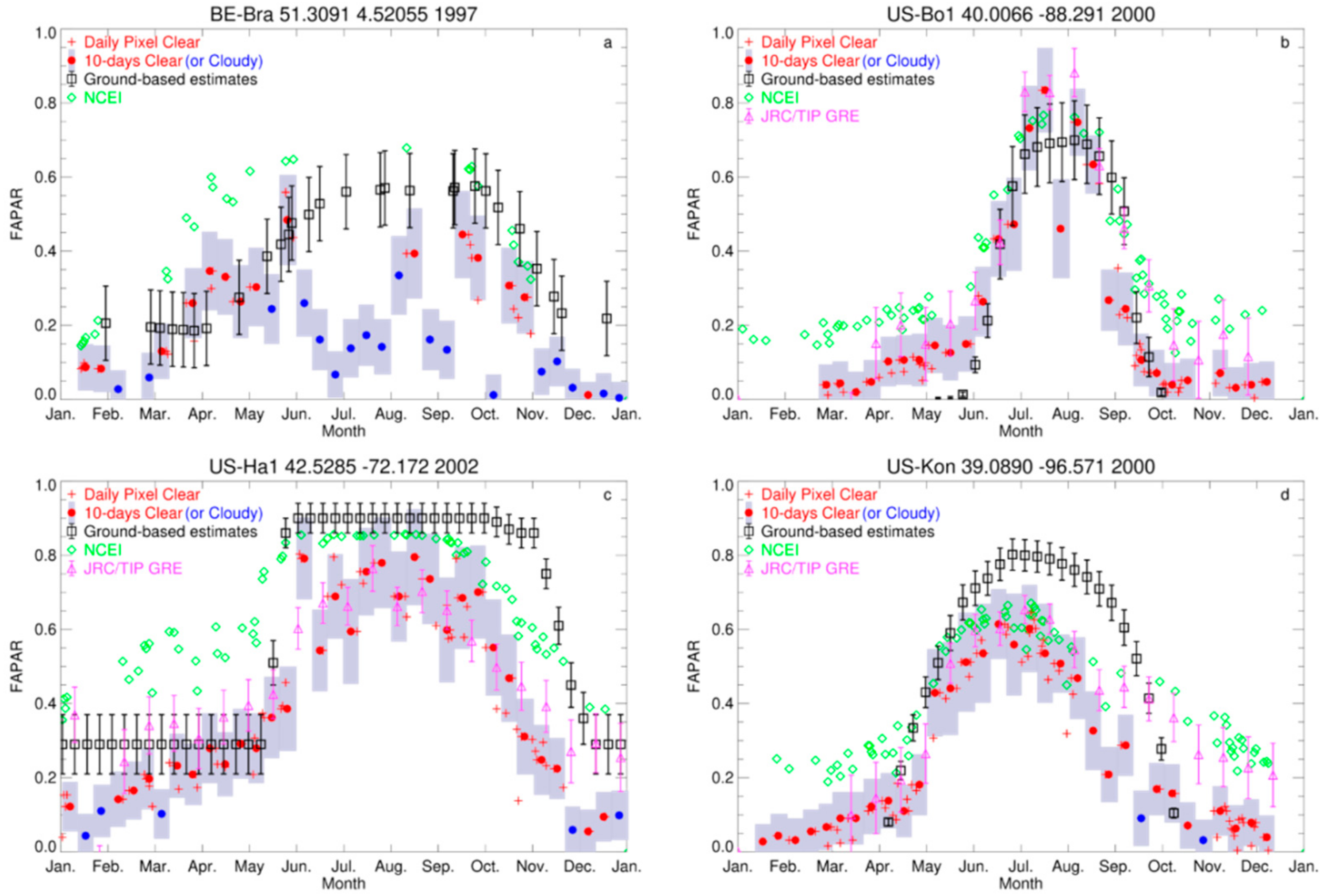
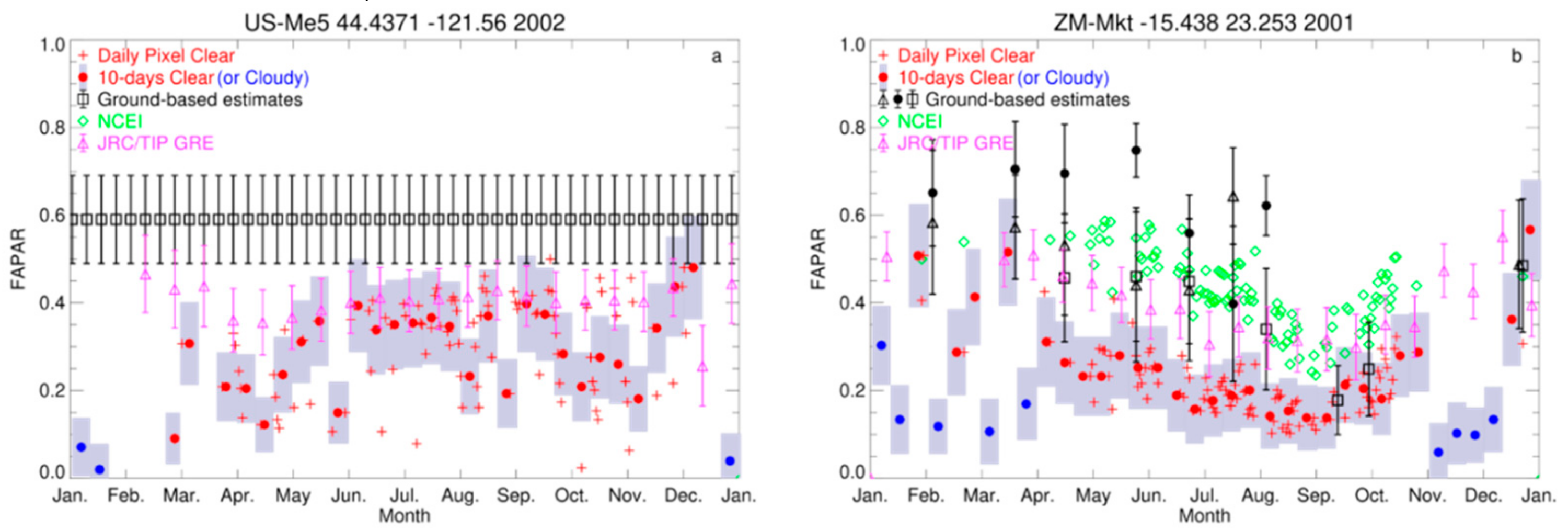
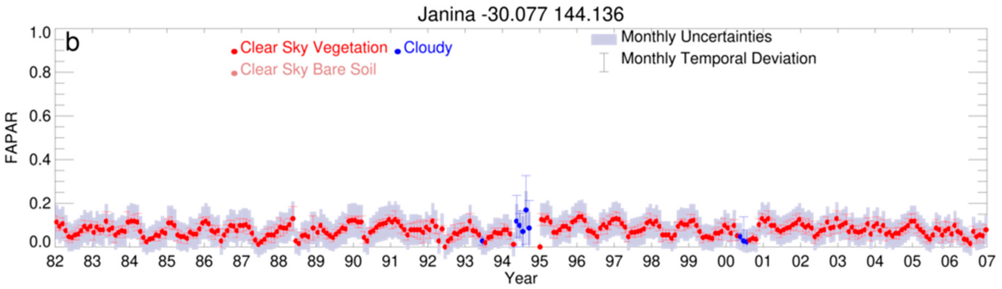
4.1. Validation Using Ground-Based Measurements

Figure 1 displays the time series of FAPAR space products together with ground-based estimates available from three sites located in Senegal, i.e., SE-Dhr (15.366°N, −15.432°E), SE-Dhr_North (15.402°N, −15.432°E), and SN-Tes (15.883°N, −15.05°E), and one at Sevilletta, USA, i.e., US-Seg (34.35°N, −106.69°E). These time series were associated with the radiation transfer in “regime 1” corresponding to the “fast” variability category. The QA4ECV product flag is indicated in red (blue) colour, when a vegetation (cloud) condition was detected, whereas the grey shade indicates temporal deviation. Ground-based estimates are plotted in black. The FAPAR baseline values over these sites are very low, and signatures of the different vegetation phenological cycles (for both the growing and senescence periods) were remarkably well-identified by both space and ground-based estimates. Moreover, the amplitudes, both the maxima and the minima, are in very good agreement amongst all products, although the space retrievals tended to slightly underestimate the ground-based values over SN-Dhr during the peak growing season (Figure 1a). Indeed, at this site, the landscape exhibited significant spatial heterogeneity not sampled by the ground-based measurements. NCEI values are slightly higher than the values of QA4ECV and JRC-TIP products, especially over the desert grassland (panel d). This may be due to leaf colour assumption differences. Pinty et al. (2011) [31] illustrated that the assumption of green leaf resulted in low values in FAPAR. These differences were limited to a range from 0.05 to 0.20 as a function of vegetation’s density. Indeed, the green hypothesis implies that a limited amount of scattering material, i.e., relatively low LAI values, is needed to match the observed data in the near-infrared band. At the same time, since the interception process mainly controlled the fraction absorbed in the visible band, relatively low LAI values in turn imposed a lower fraction of the radiation absorbed in the canopy layer. Both the JRC-TIP and QA4ECV-FAPAR products agree well with each other within their respective uncertainties.
The results over vegetation conditions belonging to the “slow variability” category, i.e., radiation transfer in “regime 2”, are displayed in Figure 2. In the case of the BE-Bra site (51.309°N, 4.52°E) (panel a), the amplitudes during the start and the end of the growing season estimated from remote sensing and ground-based measurements are in very good agreement, except for the QA4ECV results, as a lot of cloud contamination is present (blue dots). The estimated ground-based FAPAR values over the agricultural field site identified as US-Bo1 (40.006°N, −88.29°E) follow a well-defined pattern that was correctly measured by the QA4ECV products and the JRC-TIP (panel b). NCEI daily values reveal higher levels than other measurements from January up to June and after September. The third comparison performed with “regime 2” canopy conditions was conducted at the Harvard site (identified as US-Ha1), which is a mixture of conifer and hardwood forests (panel c). JRC-TIP and QA4ECV datasets were compared very well with each other including during the growing period. During the summer season, all space products then systematically showed lower values compared to those of the ground-based estimations, where vegetation got very dense. The largest differences occurred during the senescent period, where a time delay of about one month was observed between the FAPAR signatures given by space and ground-based datasets.
Both remote sensing and ground-based estimations of FAPAR over the US-Kon tall-grass prairie site (39.089°N, −96.571°E) indicated the occurrence of a pronounced vegetation seasonal cycle (panel d). JRC-TIP and QA4ECV estimations were well correlated along the cycle, although the QA4ECV products had a slightly lower bias at the end of the period. In these two sites, the bias occurring during the period of senescence was a consequence of using total (in ground-based estimations), instead of green (as assumed in the retrieval algorithm), values when assessing the FAPAR values.
The comparison results of ground-based and space-retrieved FAPAR over the US-Me5 site (44.437°N, −121.56°E), associated with “regime 3” are shown in Figure 3a. The two main interesting findings are as following: (1) neither source of information indicated a strong seasonal cycle, as could be expected over a pine conifer forest; and (2) the discrepancy in the FAPAR amplitudes between space and ground-based datasets was extremely high (by a factor of nearly 2). Both JRC-TIP and QA4ECV products showed the same amplitude of values, whereas NCEI did not provide any values. This is indeed a typical class of vegetated canopies deviating significantly from 1D statistically homogeneous situations. In this instance, the classical Beer–Bouguer–Lambert (BBL) law of exponential attenuation applies, only if the 3D radiative effects are adequately parameterized, which is not the case in the ground-based measurements.
The additional ground-based dataset associated with “regime 3” is over ZM-Mkt (–15.438°N, 23.253°E), derived from a collection and an analysis of the canopy gap fraction using the Tracing Radiation and Architecture of Canopies (TRAC) instrument in a mixed shrubland/woodland environment [20]. This instrument measures the canopy “gap size” distribution and the canopy “gap fraction” from radiation transmittance. These data provide a proxy for FAPAR, as they are used to derive the FIPAR. Figure 3b shows the time series of the FAPAR space products in 2001 together with the three transects of measurements (FIPAR spatial averages with associated standard deviations) collected by the TRAC instrument. The agreement between NCEI values and ground-based estimations is good, despite the spatial scale differences. QA4ECV-FAPAR products had lower systematical biases by about 0.2 on average during the two dry seasons. However, we have a high correlation between the two estimations. During the second wet season, we obtained opposite results of NCEI products in situ overestimate, whereas QA4ECV results were closer. It should be recalled that the contamination of the FIPAR measurements by the wooden elements of the canopy favours a bias towards green absorption values. This characteristic is higher during dry seasons, when the relative contribution to the leaf-only absorption process decreases, especially with such a sparse vegetation cover.

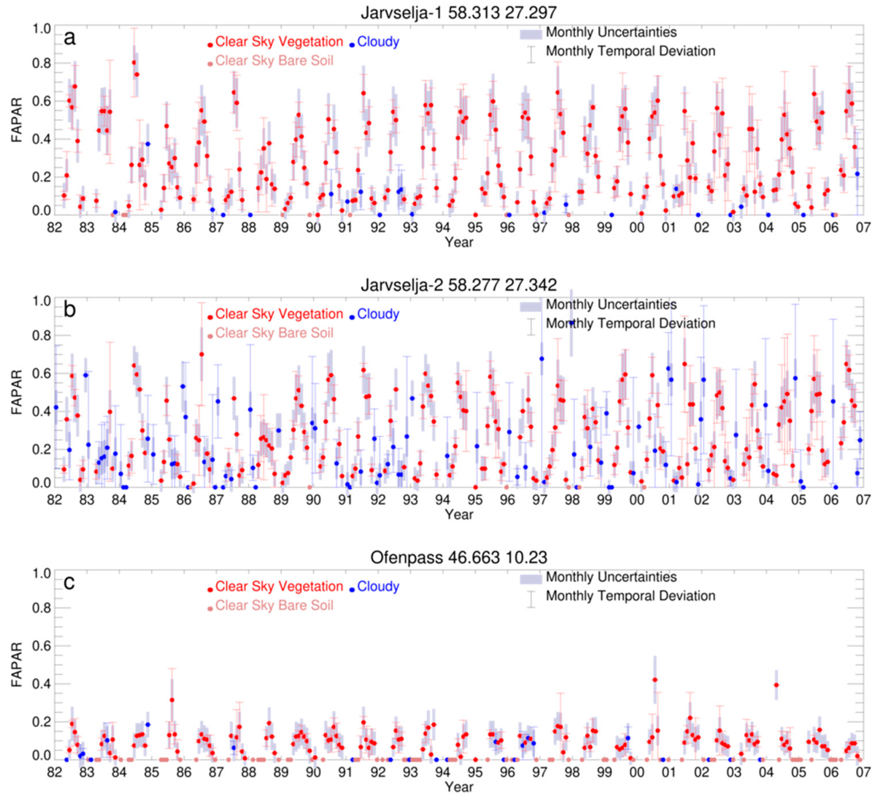
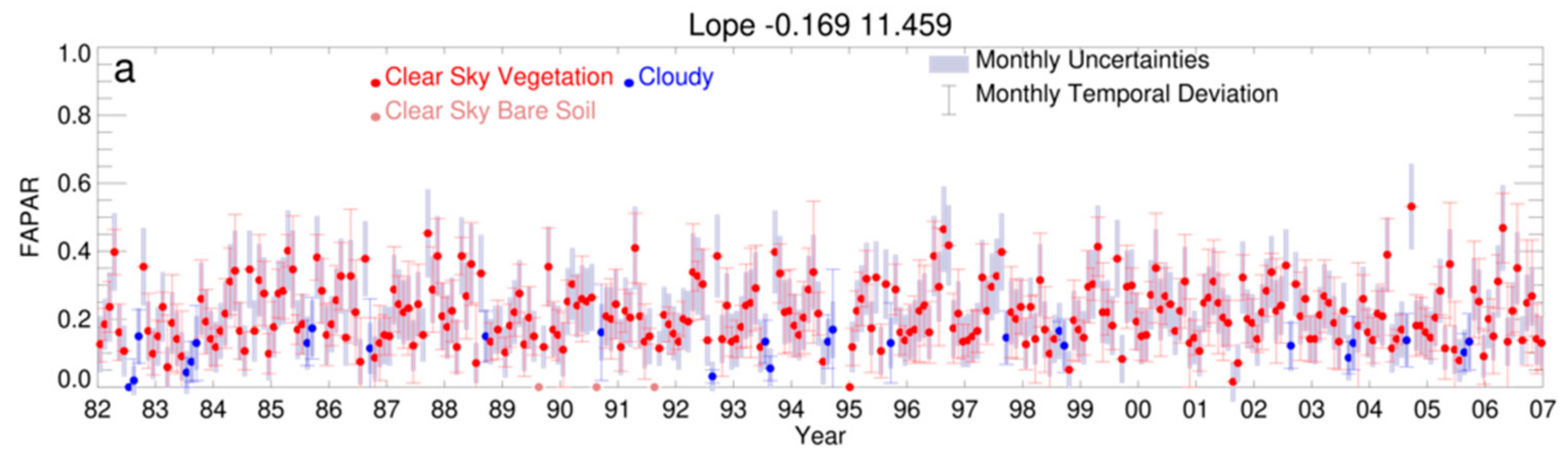
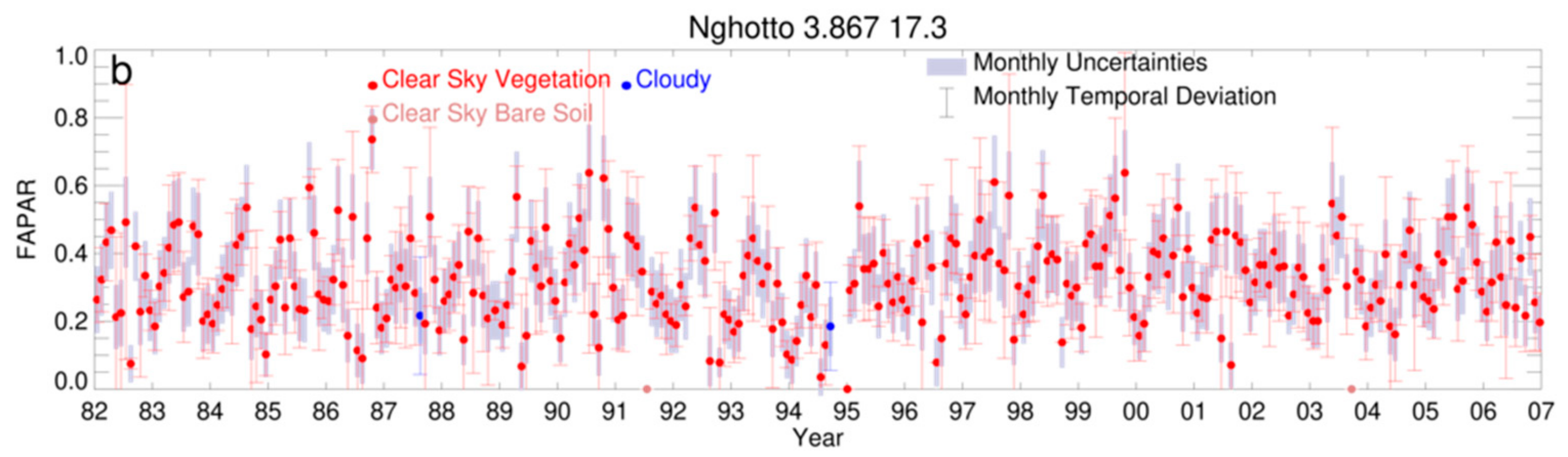
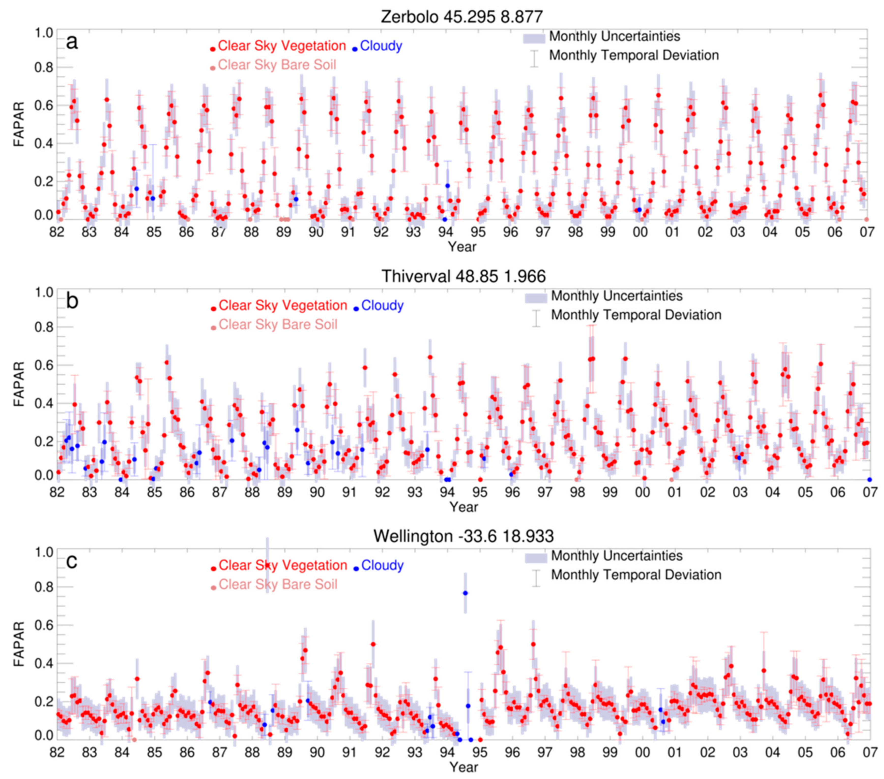
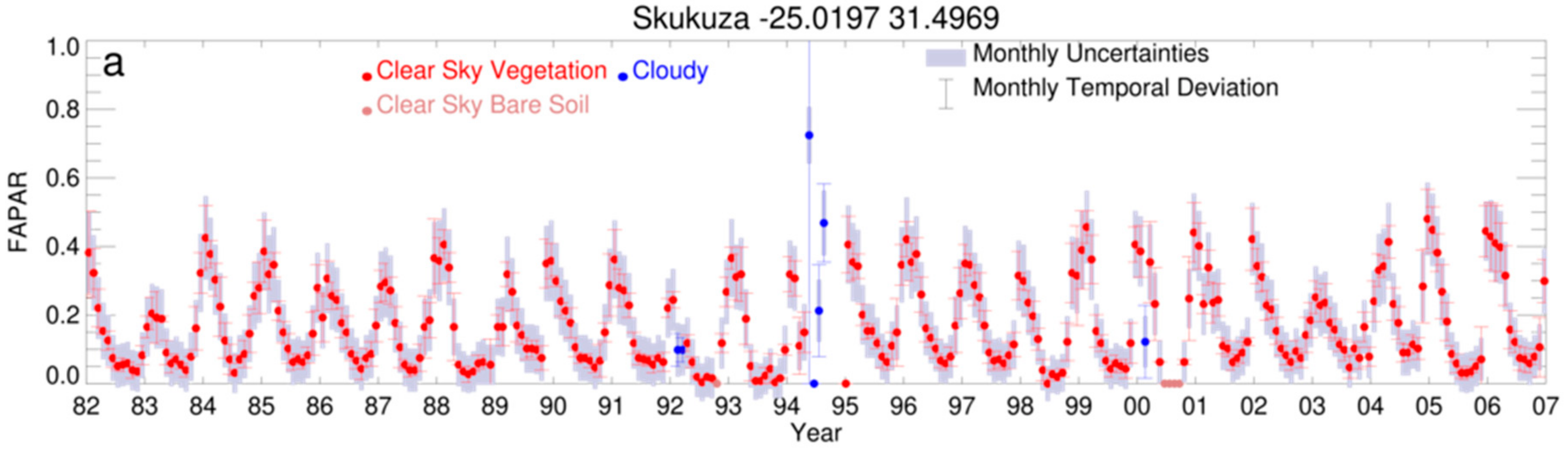
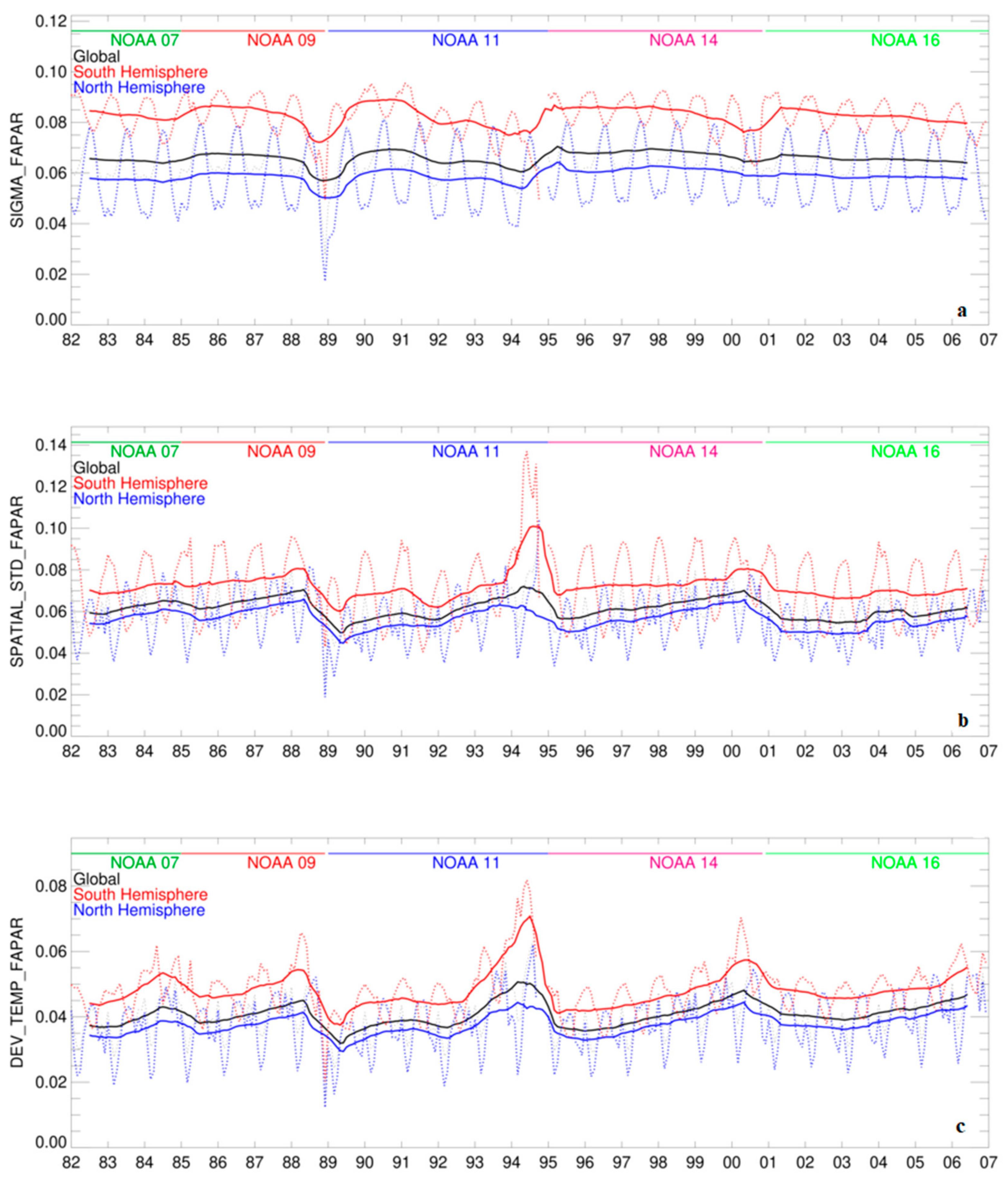
4.2. Quality Control of Monthly Time Series over 1982–2006

We presented here the time series of AVHRR-FAPAR monthly products at 0.05° × 0.05° over the QA4ECV validation sites for different types of land cover shown in Table 3.
The time series of birch stand/pine stand forests sites are plotted in Figure 4. Red (pink) dots correspond to QA4ECV best representative FAPAR best representative values at vegetation (soil) pixels. Blue symbols indicate an NCEI cloud flag, meaning that no clear sky days were found during the time composite period. Shade bars indicate the uncertainties of the best representative day, whereas error bars represent the temporal standard deviations during a month. The intra-annual seasonalities from 1982 to 2006 are in general well-represented, except for a few months, for which outliers were detected. The level of FAPAR over Ofenpass was very low compared to that of Jarvselja-2, even though both were covered by pine stand forests. The theoretical range of FAPAR that was expected over pine-stand summer (winter) virtual scenes across Ofenpass varied from 0.3 (0.2) to 0.6 (0.3), depending on the sun zenith angles (not shown here). Over Jarvselja-1, slightly higher values were obtained. During the Northern Hemisphere winter seasons, brighter surfaces were detected over this site, resulting in null FAPAR values. Over Jarvselja-2, QA4ECV monthly products still contained a lot of data contaminated by clouds, especially during winter seasons. The two tropical forest sites’ results are plotted in Figure 5.
The FAPAR values over the Lope forest are lower when compared to those for Nghotto, and their respective maxima are 0.4 and 0.6. However, it was shown that when the JRC-AVHRR retrieval algorithm was applied to simulate surface reflectance, outputs were much higher than with real data, which means that atmospheric correction may suffer from cloud contamination at the 0.05° × 0.05° scale as is often the case over these tropical regions [23].
FAPAR time series over three different types of crops are displayed in Figure 6. Panel a shows time series over the Zerbolo site covered by a short rotation poplar forest. Panels b and c correspond to wheat (Thiverval) and citrus orchard (Wellington) crops, respectively. Over this latter site, few outliers appeared, one in 1988 and some in 1994, when input data suffered from three months of missing artefacts in the Southern Hemisphere. One can notice that the products represent very well the expected seasonality for crops each year, with a high level of about 0.7 during summer over Zerbolo.
FAPAR time series over shrub and savanna sites, Skukuza and Janina, are displayed in Figure 7. Over both sites, few outliers appear for three months due to corrupted input data in 1994, for which only one-day results are available (indicated by the absence of error bars). The overall seasonality of both types of vegetation is well-represented over the entire period.

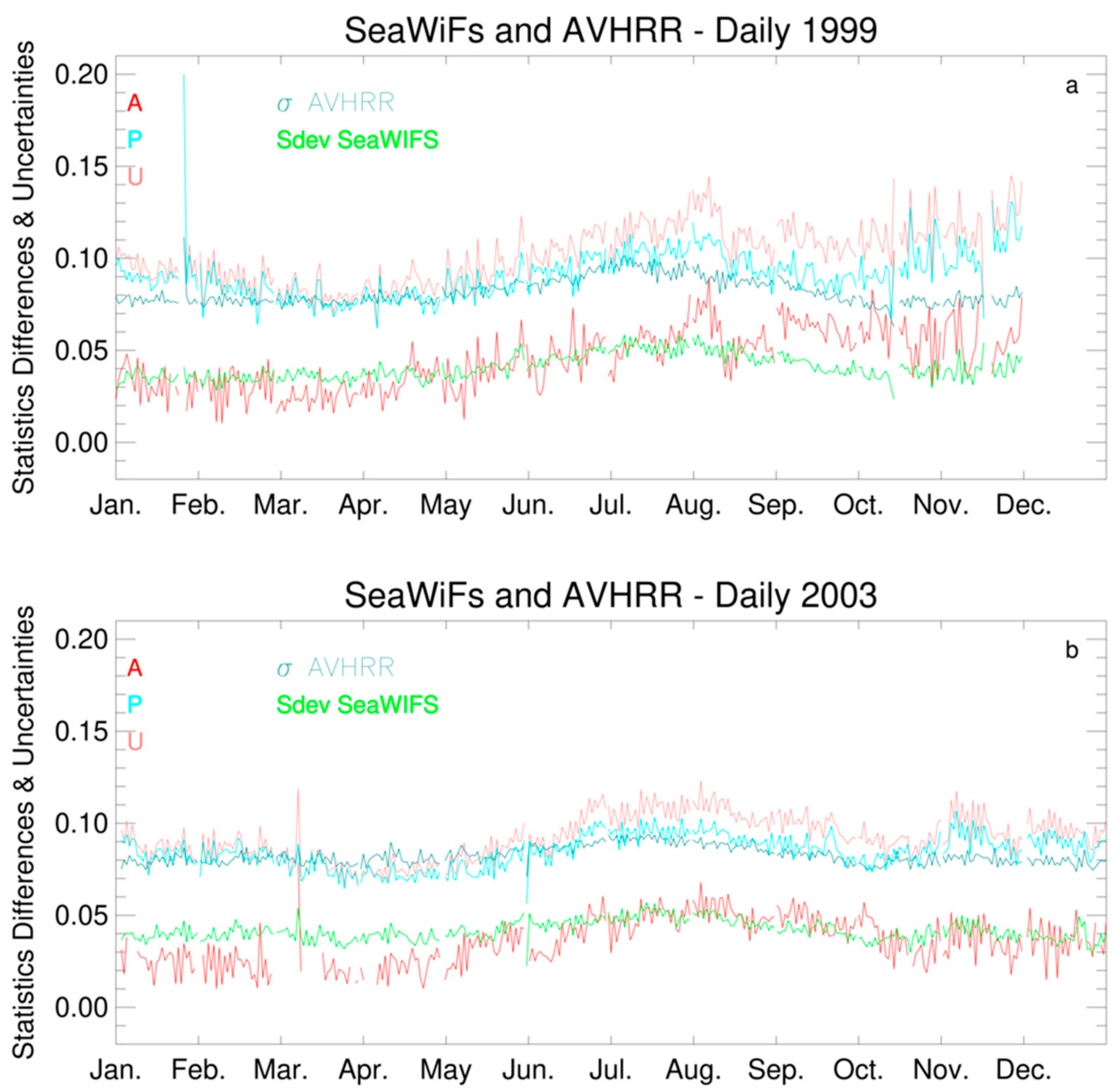
4.3. Daily Products at 0.05° × 0.05°

This section presents the comparison between QA4ECV and SeaWiFS daily products at 0.05° × 0.05° for 1999 and 2003. SeaWiFS products were derived using the same FAPAR retrieval method except that the inputs are the top of atmosphere measurements [19,23]. In order to minimise the impact of the remaining cloud effects in the SeaWiFS aggregated products, data were filtered by keeping only grid cells that contained less than 50% of cloudy pixels. Daily comparison statistics at a global scale are reported in Figure 8. A and U values are plotted in red and pink lines, respectively. In addition, the SeaWiFS spatial standard deviation, Sdev, is displayed in green, whereas the QA4ECV uncertainty, σ, is in blue. We can see that, for 1999 (panel a) and 2003 (panel b), A (U) values are lower than 0.05 (0.10) until July but increase afterwards. U values are smaller or of the same order compared to the actual uncertainties of FAPAR. (A, P, U) are higher in 1999 compared to those in 2003. This may be due to calibration differences of instruments between the NOAA14 (AVHRR2) and NOAA16 (AVHRR3) platforms.

4.4. Monthly Products at 0.5° × 0.5°

This subsection informs on the mean average bias between SeaWiFS and QA4ECV monthly products at 0.5° × 0.5° over the 1998–2005 period. Figure 9a presents longitudinal averages of these differences (reddish/blueish colours showing negative/positive values). SeaWiFS values are lower during the vegetation peak season in the Southern Hemisphere, as it contains many small vegetated canopies, such as in Australia and Southern Africa. For the other places, we can see that SeaWiFS values are often higher than QA4ECV values, especially at the end of 2000 around the equator. Figure 9b presents the density scatter plots of two sensors’ products, and Figure 9c shows the histogram of differences using 8-year data. We found that the mean average difference δ is at 0.0755 with a mean deviation of 0.091. We propose a linear bias correction for each month at grid level as explained in Section 3. The comparisons following this correction are displayed in Figure 10, where the mean average difference δ drops to 0.0011 and the mean deviation reduces to 0.0249. The longitudinal plot (panel a) shows that the absolute agreement is on average less than 0.10.

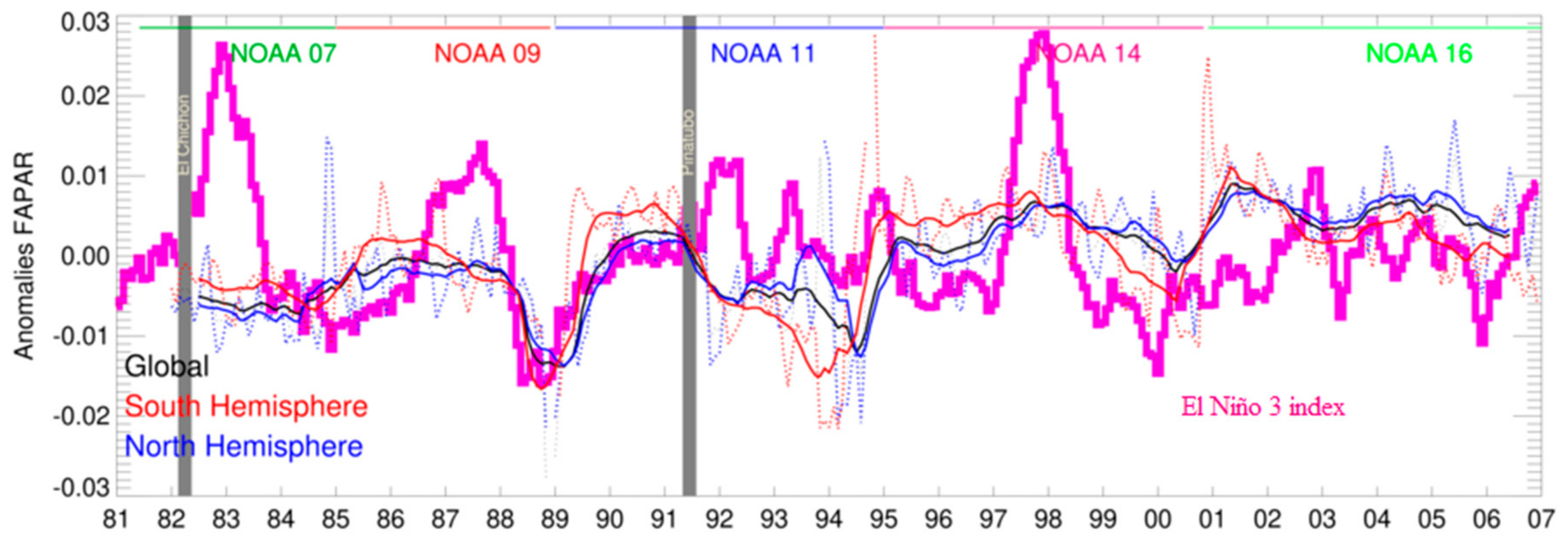
4.5. Global Change Studies: Impact of Calibration

This subsection discusses the level of confidence when using long-term time series for global change studies, as done in the state of climate reports [47,48]. The quality of the AVHRR data was first evaluated by examining the stability of the rectified channels in bands 1 and 2 during the entire period over the CEOS Libya-4 bright calibration site (28.55°N, 23.29°E).
One can easily see some artefacts during the period, especially in the near-infrared (band 2) (Figure 11b). These occurred at the end of 1984, 1987, 1988, 1993, and 2000, and afterwards, the values are more stable. The reasons for this instability concern principally the difficulty of calibration of old sensors and sensor drifts. Previous AVHRR land products suffer from these defects as shown in [13].
The stability of climate data records can be also checked with the time series of uncertainties. Figure 12 displays the three uncertainties provided in the QA4ECV monthly products at 0.5° × 0.5° averaged at a global scale and over the two hemispheres, respectively. We observed that the uncertainties values, σ, are lower than 0.1 (panel a). Both the spatial and temporal standard deviation plots also revealed the nonstability that was found in the previous analysis. These results indicated that we can filter products by applying a total uncertainties threshold.
We also needed to take into account the actual number of grid cells that constituted the global mean for each period that could increase or decrease this global average. In Figure 13, we plotted the global and the Northern/Southern Hemispheres FAPAR anomalies from 1982 to 2006 (using linear-bias-corrected QA4ECV data). It should be noted that, for the spatial average, we removed grid cells, of which either one of the uncertainties or the total was above 0.20. We also removed monthly values, where the number of pixels used for the spatial average was less than 50% of the climatology of the number of pixels.
Figure 13 displays the global and Northern/Southern Hemispheres FAPAR monthly anomalies from 1982 to 2006. Dotted lines correspond to monthly values, whereas solid lines indicate 6-month running averages. The pink histogram indicates the El Niño 3 index anomalies over the same period. The El Niño 3 index corresponds to the area-averaged sea surface temperature (SST) from 5°S to 5°N and from 150°W to 90°W [49,50]. The extreme negative anomaly occurred at the end of 1988 after the 1987 El Niño event, but this result should be interpreted with caution, as it was also at the end of life of the NOAA-09 instrument. The Pinatubo eruption played a strong role with respect to land precipitation and associated drought conditions in 1992 that are evidenced with a negative FAPAR anomaly. More recently, after the strong El Niño event in 1997, one can see that the negative FAPAR anomaly extended until the start of 2001 as was already shown in [51]. Afterwards, the anomalies became positive, and a small positive trend was detectable.

5. Conclusions

This paper presented the performance assessment of the QA4ECV black-sky FAPAR long-term records at different spatial and temporal scales, i.e., at 0.05° × 0.05° and 0.5° × 0.5° for daily, 10-day and monthly periods. Validation was done through comparisons against time series of ground-based estimates, together with NCEI products and JRC-TIP, using a categorization of the ground-based FAPAR datasets according to their most probable radiative transfer regimes. Despite the spatial-scale differences between these ground-based measurements and space products, we found out a relatively good agreement of radiative transfer in “regime 1” and “regime 2”. These past ground-based measurements are, however, only a proxy of FAPAR space products, as they represented the interception rather than the actual absorption by green leaves. Progresses in making better reference validation measurements are ongoing within the European Space Agency (ESA) Fiducial Reference Measurements for Vegetation project (https://frm4veg.org/) that will provide traceable in situ measurements. In addition, the Ground-Based Observations for Validation (GBOV) component of the Copernicus Global Land Products (https://land.copernicus.eu/global/gbov) provides multiyear ground-based observations from existing global networks. However, these projects cannot provide data prior to 2016. Over the QA4ECV virtual validation sites, monthly products at 0.05° × 0.05° were used from 1982 to 2006 to check inter-annual variations and stability and to identify outliers. These results could be useful for further AVHRR calibration improvements and artefact detection.
We also compared the QA4ECV global daily products against SeaWiFS for 1999 and 2003 at 0.05° × 0.05°. Both bias and root mean square deviation (RMSD) were reported together with QA4ECV FAPAR uncertainties and the spatial standard deviation of SeaWiFS. We found larger differences in 1999 compared to those in 2003, because the AVHRR-2 and AVHRR-3 instruments have different calibration features. However, these statistical values were within the product uncertainties. Monthly products at 0.5° × 0.5° between SeaWiFS and QA4ECV were also benchmarked, and we demonstrated that a monthly linear correction can be used for correcting the entire QA4ECV time series, from 1982 onwards, for correcting the stability performance. Recently, Giering, et al. (2019) proposed a framework to establish fundamental satellite data series for climate applications [52]. Here, we applied a simple approach that can bring a solution for merging different sensor products.
We analysed the products over terrestrial surfaces at a global scale as was done in [48,53]. We identified the global changes of terrestrial surfaces that should be interpreted with care because of the instability of AVHRR data. This dataset could be easily extended with products from MERIS, “green” JRC-TIP and Sentinel-3 OLCI, as they represent the same variable. More work is required to explore these data as well as geostationary ones to increase the number of available productive climate data records.

Author Contributions

N.G. conceived, designed and implemented the JRC-AVHRR algorithm and made the performances studies. M.M. and M.R. contributed to the data processing. N.G. wrote the paper. E.V. contributed to the availability of an improved surface reflectance within the QA4ECV project.

Acknowledgments

This research was funded by the European Union FP7 Project—Quality Assurance for Essential Climate Variables (QA4ECV) (grant No.: 607405). The support provided by the European Commission Directorate-General for Internal Market, Industry, Entrepreneurship and SMEs and Copernicus Programme is gratefully acknowledged. The authors thank the two anonymous reviewer’s comments. The first author thanks Olivier Morgan for his proofreading.

Conflicts of Interest

The authors declare no conflicts of interest.

References

  1. Sellers, P.J.; Dickinson, R.E.; Randall, D.A.; Betts, A.K.; Hall, F.G.; Berry, J.A.; Collatz, G.J.; Denning, A.S.; Mooney, H.A.; Nobre, C.A.; et al. Modeling the Exchanges of Energy, Water, and Carbon Between Continents and the Atmosphere. Science 1997, 275, 502–509. [Google Scholar] [CrossRef] [Green Version]
  2. Knyazikhin, Y.; Martonchik, J.V.; Myneni, R.B.; Diner, D.J.; Running, S.W. Synergistic algoritm for estimating vegetation canopy leaf area index and fraction of absorbed photosynthetically active radiation from MODIS and MISR data. Geophys. Res. 1998, 103, 32257–32276. [Google Scholar] [CrossRef] [Green Version]
  3. Disney, M.; Muller, J.P.; Kharbouche, S.; Kaminski, T.; Vossbeck, M.; Lewis, P.; Pinty, B. A New Global fAPAR and LAI Dataset Derived from Optimal Albedo Estimates: Comparison with MODIS Products. Remote Sens. 2016, 8, 275. [Google Scholar] [CrossRef] [Green Version]
  4. Chernetskiy, M.; Gómez-Dans, J.; Gobron, N.; Morgan, O.; Lewis, P.; Truckenbrodt, S.; Schmullius, C. Estimation of FAPAR over Croplands Using MISR Data and the Earth Observation Land Data Assimilation System (EO-LDAS). Remote Sens. 2017, 9, 656. [Google Scholar] [CrossRef] [Green Version]
  5. Knorr, W.; Kaminski, T.; Scholze, M.; Gobron, N.; Pinty, B.; Giering, R.; Mathieu, P.P. Carbon Cycle Data Assimilation with a Generic Phenology Model. J. Geophys. Res. Biogeosci. 2010, 115, G04017. [Google Scholar] [CrossRef] [Green Version]
  6. Kaminski, T.; Knorr, W.; Scholze, M.; Gobron, N.; Pinty, B.; Giering, R.; Mathieu, P.P. Consistent assimilation of MERIS FAPAR and atmospheric CO2 into a terrestrial vegetation model and interactive mission benefit analysis. Biogeosciences 2012, 9, 3173–3184. [Google Scholar] [CrossRef] [Green Version]
  7. Wu, M.; Scholze, M.; Vossbeck, M.; Kaminski, T.; Hoffmann, G. Simultaneous Assimilation of Remotely Sensed Soil Moisture and FAPAR for Improving Terrestrial Carbon Fluxes at Multiple Sites Using CCDAS. Remote Sens. 2018, 11, 27. [Google Scholar] [CrossRef] [Green Version]
  8. Peng, J.; Muller, J.P.; Blessing, S.; Giering, R.; Danne, O.; Gobron, N.; Kharbouche, S.; Ludwig, R.; Muller, B.; Leng, G.; et al. Can We Use Satellite-Based FAPAR to Detect Drought? Sensors 2019, 19, 3662. [Google Scholar] [CrossRef] [Green Version]
  9. Pfeifer, M.; Disney, M.; Quaife, T.; Marchant, R. Terrestrial ecosystems from space: A review of earth observation products for macroecology applications. Glob. Ecol. Biogeogr. 2012, 21, 603–624. [Google Scholar] [CrossRef] [Green Version]
  10. Ceccherini, G.; Gobron, N.; Migliavacca, M. On the Response of European Vegetation Phenology to Hydroclimatic Anomalies. Remote Sens. 2014, 6, 3143–3169. [Google Scholar] [CrossRef] [Green Version]
  11. GCOS. The Global Observing System for Climate: Implementation Needs; Technical Report GCOS-200; World Meteorological Organization: Geneva, Switzerland, 2003. [Google Scholar]
  12. GCOS. Summary Report of the Eleventh Session of the WMO-IOC-UNEP-ICSU (WMO/TD-No.1189); Report Melbourne, Australia, April 7–10 GCOS-87; World Meteorological Organization: Geneva, Switzerland, 2016. [Google Scholar]
  13. Zhu, Z.; Bi, J.; Pan, Y.; Ganguly, S.; Anav, A.; Xu, L.; Samanta, A.; Piao, S.; Nemani, R.R.; Myneni, R.B. Global Data Sets of Vegetation Leaf Area Index (LAI)3g and Fraction of Photosynthetically Active Radiation (FPAR)3g Derived from Global Inventory Modeling and Mapping Studies (GIMMS) Normalized Difference Vegetation Index (NDVI3g) for the Period 1981 to 2011. Remote Sens. 2013, 5, 927–948. [Google Scholar] [CrossRef] [Green Version]
  14. Claverie, M.; Matthews, J.L.; Vermote, E.F.; Justice, C.O. A 30+ Year AVHRR LAI and FAPAR Climate Data Record: Algorithm Description and Validation. Remote Sens. 2016, 8, 263. [Google Scholar] [CrossRef] [Green Version]
  15. Xiao, Z.; Liang, S.; Wang, T.; Jiang, B. Retrieval of Leaf Area Index (LAI) and Fraction of Absorbed Photosynthetically Active Radiation (FAPAR) from VIIRS Time-Series Data. Remote Sens. 2016, 8, 351. [Google Scholar] [CrossRef] [Green Version]
  16. Xiao, Z.; Liang, S.; Sun, R. Evaluation of Three Long Time Series for Global Fraction of Absorbed Photosynthetically Active Radiation (FAPAR) Products. IEEE Trans. Geosci. Remote Sens. 2018, 1–16. [Google Scholar] [CrossRef]
  17. Franch, B.; Vermote, E.F.; Roger, J.C.; Murphy, E.; Becker-Reshef, I.; Justice, C.; Claverie, M.; Nagol, J.; Csiszar, I.; Meyer, D.; et al. A 30+ Year AVHRR Land Surface Reflectance Climate Data Record and Its Application to Wheat Yield Monitoring. Remote Sens. 2017, 9, 296. [Google Scholar] [CrossRef] [Green Version]
  18. Nightingale, J.; Boersma, K.F.; Muller, J.P.; Compernolle, S.; Lambert, J.; Blessing, S.; Giering, R.; Gobron, N.; De Smedt, I.; Coheur, P.; et al. Quality Assurance Framework Development Based on Six New ECV Data Products to Enhance User Confidence for Climate Applications. Remote Sens. 2018, 10, 1254. [Google Scholar] [CrossRef] [Green Version]
  19. Gobron, N.; Pinty, B.; Mélin, F.; Taberner, M.; Verstraete, M.M. Sea Wide Field-of-View Sensor (SeaWiFS)—An Optimized FAPAR Algorithm—Theoretical Basis Document; European Commission, Institute for Environment and Sustainability: Ispra, Italy, 2002. [Google Scholar]
  20. Gobron, N.; Aussédat, O.; Pinty, B.; Taberner, M.; Verstraete, M.M. Medium Resolution Imaging Spectrometer (MERIS)—Level 2 Land Surface Products—Algorithm Theoretical Basis Document-Revision 3.0; EUR Report No. 21387 EN; European Commission, Institute for Environment and Sustainability: Ispra, Italy, 2004. [Google Scholar]
  21. Gobron, N. Envisat’s Medium Resolution Imaging Spectrometer (MERIS) Algorithm Theoretical Basis Document: FAPAR and Rectified Channels Over Terrestrial Surfaces. Eur. Rep. 2011, 24844. [Google Scholar] [CrossRef]
  22. Gobron, N. Ocean and Land Colour Instrument (OLCI) FAPAR and Rectified Channels Over Terrestrial Surfaces Algorithm Theoretical Basis Document; Technical Report; Institute for Environment and Sustainability, European Commission: Brussels, Belgium, 2011. [Google Scholar]
  23. Gobron, N.; Pinty, B.; Aussedat, O.; Chen, J.M.; Cohen, W.B.; Fensholt, R.; Gond, V.; Huemmrich, K.F.; Lavergne, T.; Mélin, F.; et al. Evaluation of FAPAR Products for Different Canopy Radiation Transfer Regimes: Methodology and Results using JRC Products Derived from SeaWiFS against ground-based estimations. J. Geophys. Res. Atmos. 2006, 111. [Google Scholar] [CrossRef]
  24. Tao, X.; Liang, S.; Wang, D. Assessment of five global satellite products of fraction of absorbed photosynthetically active radiation: Intercomparison and direct validation against ground-based data. Remote Sens. Environ. 2015, 163, 270–285. [Google Scholar] [CrossRef]
  25. Gobron, N.; Pinty, B.; Aussédat, O.; Taberner, M.; Faber, O.; Mélin, F.; Lavergne, T.; Robustelli, M.; Snoeij, P. Uncertainty estimates for the FAPAR operational products derived from MERIS—Impact of top-of-atmosphere radiance uncertainties and validation with field data. Remote Sens. Environ. 2008, 112, 1871–1883. [Google Scholar] [CrossRef]
  26. Gobron, N.; Dash, J.; Lopez Baeza, E.; Cescatti, A.; Gitelson, A.; Gruening, C.; Schmullius, C.; Widlowski, J.L. SENTINEL-3 Ocean Land Color Imager (OLCI): Land products and Validation. In Proceedings of the 2013 ESA Living Planet Symposium, Edinburgh, UK, 9–13 September 2013. [Google Scholar]
  27. Gobron, N.; Morgan, O.; Adams, J.; Brown, L.; Dash, J.; Lanconnelli, J.; Marioni, M.; Robustelli, M.; Suyker, A.E. Evaluation of Sentinel-3A and Sentinel-3B OLCI FAPAR. Remote Sens. 2020. in preparation. [Google Scholar]
  28. Zhu, Z.; Piao, S.; Myneni, R.B.; Huang, M.; Zeng, Z.; Canadell, J.G.; Ciais, P.; Sitch, S.; Friedlingstein, P.; Arneth, A.; et al. Greening of the Earth and its drivers. Nat. Clim. Chang. 2016, 6, 791–795. [Google Scholar] [CrossRef]
  29. Jiang, C.; Ryu, Y.; Fang, H.; Myneni, R.; Claverie, M.; Zhu, Z. Inconsistencies of interannual variability and trends in long-term satellite leaf area index products. Glob. Chang. Biol. 2017, 23, 4133–4146. [Google Scholar] [CrossRef] [PubMed]
  30. Claverie, M.; Vermote, E. NOAA Climate Data Record (CDR) of Leaf Area Index (LAI) and Fraction of Absorbed Photosynthetically Active Radiation (FAPAR), Version 4; NOAA National Centers for Environmental Information: Washington, DC, USA, 2014. [CrossRef]
  31. Pinty, B.; Andredakis, I.; Clerici, M.; Kaminski, T.; Taberner, M.; Verstraete, M.M.; Gobron, N.; Plummer, S.; Widlowski, J.L. Exploiting the MODIS albedos with the Two-stream Inversion Package (JRC-TIP): 1. Effective leaf area index, vegetation, and soil properties. J. Geophys. Res. Atmos. 2011, 116. [Google Scholar] [CrossRef]
  32. Lanconelli, C.; Gobron, N.; Adams, J.; Danne, O.; Blessing, S.; Robustelli, M.; Kharbouche, S.; Muller, J.P. Report on the Quality Assessment of Land ECV Retrieval Algorithms; Scientific and Technical Report JRC109764; European Commission, Joint Research Centre: Ispra, Italy, 2018. [Google Scholar]
  33. Gobron, N.; Adams, J.; Brennan, J.; Disney, M.; Govaerts, Y.; Mio, C. QA4ECV: Descriptions of Virtual Validation Sites; Report JRC97694; European Commission: Brussels, Belgium, 2015. [Google Scholar]
  34. Vermote, E. NOAA Climate Data Record (CDR) of AVHRR Surface Reflectance, Version 5. NOAA National Centers for Environmental Information: Washington, DC, USA, 2019. [Google Scholar] [CrossRef]
  35. Huemmrich, K.F.; Privette, J.L.; Mukelabai, M.; Myneni, R.B.; Knyazikhin, Y. Time-series Validation of MODIS Land Biophysical Products in a Kalahari Woodland, Africa. Int. J. Remote Sens. 2005, 26, 4381–4398. [Google Scholar] [CrossRef]
  36. Wang, Y.; Woodcock, C.E.; Buermann, W.; Stenberg, P.; Voipio, P.; Smolander, H.; Hame, T.; Tian, Y.; Hu, J.; Knyazikhin, Y.; et al. Evaluation of the MODIS LAI Algorithm at a Coniferous Forest Site in Finland. Remote Sens. Environ. 2004, 91, 114–127. [Google Scholar] [CrossRef]
  37. Shabanov, N.V.; Wang, Y.; Buermann, W.; Dong, J.; Hoffman, S.; Smith, G.R.; Tian, Y.; Knyazikhin, Y.; Myneni, R.B. Effect of Foliage Spatial Heterogeneity in the MODIS LAI and FPAR Algorithm over Broadleaf Forests. Remote Sens. Environ. 2003, 85, 410–423. [Google Scholar] [CrossRef] [Green Version]
  38. Davis, A.B.; Marshak, A. Photon Propagation in Heterogeneous Optical Media with Spatial Correlations: Enhanced Mean Free-paths and Wider-than-exponential Free-path Distributions. J. Quant. Spectrosc. Radiat. Transf. 2004, 84, 3–34. [Google Scholar] [CrossRef]
  39. Fensholt, R.; Sandholt, I.; Rasmussen, M.S. Evaluation of MODIS LAI, fAPAR and the relation between fAPAR and NDVI in a semi-arid environment using in situ measurements. Remote Sens. Environ. 2004, 91, 490–507. [Google Scholar] [CrossRef]
  40. Turner, D.P.; Ritts, W.D.; Cohen, W.B.; Maeirsperger, T.K.; Gower, S.T.; Kirschbaum, A.A.; Running, S.W.; Zhao, M.; Wofsy, S.C.; Dunn, A.L.; et al. Site-level evaluation of satellite-based global terrestrial gross primary production and net primary production monitoring. Glob. Chang. Biol. 2005, 11, 666–684. [Google Scholar] [CrossRef]
  41. Privette, J.; Tian, Y.; Roberts, G.; Scholes, R.; Wang, Y.; Caylor, K.; Frost, P.; Mukelabai, M. Vegetation structure characteristics and relationships of Kalahari woodlands and savannas. Glob. Chang. Biol. 2004, 10, 281–291. [Google Scholar] [CrossRef] [Green Version]
  42. Gond, V.; de Pury, D.D.D.; Veroustraete, F.; Ceulemans, R. Seasonal variations in leaf area index, leaf chlorophyll, and water content; scaling-up to estimate fAPAR and carbon balance in a multilayer, multispecies temperate forest. Tree Physiol. 1999, 19, 673–679. [Google Scholar] [CrossRef] [Green Version]
  43. Gobron, N.; Pinty, B.; Verstraete, M.M.; Govaerts, Y. A Semi-Discrete Model for the Scattering of Light by Vegetation. J. Geophys. Res. 1997, 102, 9431–9446. [Google Scholar] [CrossRef]
  44. Gobron, N. QA4ECV Algorithm Theoretical Basis Document for JRC AVHRR FAPAR; Eur Report; European Commission: Brussels, Belgium, 2017. [Google Scholar]
  45. Pinty, B.; Clerici, M.; Andredakis, I.; Kaminski, T.; Taberner, M.; Verstraete, M.M.; Gobron, N.; Plummer, S.; Widlowski, J.L. Exploiting the MODIS albedos with the Two-stream Inversion Package (JRC-TIP): 2. Fractions of transmitted and absorbed fluxes in the vegetation and soil layers. J. Geophys. Res. Atmos. 2011, 116. [Google Scholar] [CrossRef] [Green Version]
  46. Vermote, E.F.; Kotchenova, S. Atmospheric correction for the monitoring of land surfaces. J. Geophys. Res. Atmos. 2008, 113. [Google Scholar] [CrossRef]
  47. Gobron, N. [GLOBAL CLIMATE] Terrestrial vegetation dynamics [in ‘State of the Climate in 2016’]. Bull. Am. Meteorol. Soc. 2017, 98, S57. [Google Scholar] [CrossRef] [Green Version]
  48. Gobron, N. Terrestrial vegetation dynamics [in “State of the Climate in 2018”]. Bull. Am. Meteorol. Soc. 2019, 100, S63–S64. [Google Scholar] [CrossRef] [Green Version]
  49. Rayner, N.A.; Parker, D.E.; Horton, E.B.; Folland, C.K.; Alexander, L.V.; Rowell, D.P.; Kent, E.C.; Kaplan, A. Global analyses of sea surface temperature, sea ice, and night marine air temperature since the late nineteenth century. J. Geophys. Res. Atmos. 2003, 108. [Google Scholar] [CrossRef]
  50. Available online: https://www.esrl.noaa.gov/psd/gcos_wgsp/Timeseries/Nino3/ (accessed on 16 October 2019).
  51. Knorr, W.; Gobron, N.; Scholze, M.; Kaminski, T.; Schnur, R.; Pinty, B. Impact of Terrestrial Biosphere Carbon Exchanges on the Anomalous CO2 Increase in 2002–2003. Geophys. Res. Lett. 2007. [Google Scholar] [CrossRef]
  52. Giering, R.; Quast, R.; Mittaz, J.P.D.; Hunt, S.E.; Harris, P.M.; Woolliams, E.R.; Merchant, C.J. A Novel Framework to Harmonise Satellite Data Series for Climate Applications. Remote Sens. 2019, 11, 2. [Google Scholar] [CrossRef] [Green Version]
  53. Gobron, N.; Robustelli, M. Monitoring the state of the global terrestrial surfaces. In Proceedings of the 2013 ESA Living Planet Symposium, Edinburgh, UK, 9–13 September 2013. [Google Scholar]
Figure 1. Time series associated with the radiation transfer in “regime 1” (fast variability) over SE-Dhr (15.366°N, −15.432°E) (a), SE-Dhr_North (15.402°N, −15.432°E) (b), SN-Tes (15.883°N, −15.05°E) (c), and US-Seg (34.35°N, −106.69°E) (d). The QA4ECV products are plotted in red with dotted (cross) symbols for 10-day (daily) values. Blue points indicate values with the remaining cloud flags. Ground-based estimates are black squares. NCEI daily products are plotted with green diamond symbols, and JRC-TIP products are represented with pink triangles. The error (shade) bars correspond to the uncertainties of each product when available.
Remotesensing 11 03055 g001
Figure 2. Time series associated with the radiation transfer in “regime 2” (slow variability) over BE-Bra (51.309°N, 4.52°E) (a), US-Bo1 (40.006°N, −88.29°E) (b), US-Ha1 (42.52°N, −72.172°E) (c), and US-Kon (39.089°N, −96.571°E) (d). The QA4ECV products are plotted in red dotted (cross) symbols for 10-day (daily) values. Blue points indicate values with the remaining cloud flags. Ground-based estimates are black squares. NCEI daily products are plotted with green diamond symbols, and JRC-TIP products are represented with pink triangles. The error (shade) bars correspond to the uncertainties of each product when available.
Remotesensing 11 03055 g002
Figure 3. Time series associated with the radiation transfer in “regime 3” (resonant variability) over the US-Me5 site (44.437°N, −121.56°E) (a) and the ZM-Mkt site (–15.438°N, 23.253°E) (b). The QA4ECV products are plotted in red dotted (cross) symbols for 10-day (daily) values. Blue points indicate values with the remaining cloud flags. Ground-based estimates are black squares. NCEI daily products are plotted with green diamond symbols, and JRC-TIP products are represented with pink triangles. The error (shade) bars correspond to the uncertainties of each product when available.
Remotesensing 11 03055 g003
Figure 4. Time series of FAPAR monthly products over QA4ECV forest sites: (a) Jarvselha-1; (b) Jarvselha-2; and (c) Ofenpass. Red and brown dotted symbols indicate vegetation and bare soil flags, respectively, whereas blue ones indicate cloud. Error and shade bars correspond to monthly uncertainties and temporal deviations, respectively.
Remotesensing 11 03055 g004
Figure 5. Time series of FAPAR monthly products over QA4ECV tropical forest sites: (a) Lope and (b) Nghotto. Red and brown dotted symbols indicate vegetation and bare soil flags, respectively, whereas blue ones indicate cloud. Error and shade bars correspond to monthly uncertainties and temporal deviations, respectively.
Remotesensing 11 03055 g005aRemotesensing 11 03055 g005b
Figure 6. Time series of FAPAR monthly products over QA4ECV crops sites: (a) Zerbolo; (b) Thiverval; and (c) Wellington. Red and brown dotted symbols indicate vegetation and bare soil flags, respectively, whereas blue ones indicate cloud. Error and shade bars correspond to monthly uncertainties and temporal deviations, respectively.
Remotesensing 11 03055 g006
Figure 7. Time series of FAPAR monthly products over QA4ECV shrub (a) and savanna (b) sites. Red and brown dotted symbols indicate vegetation and bare soil flags, respectively, whereas blue ones indicate cloud. Error and shade bars correspond to monthly uncertainties and temporal deviations, respectively.
Remotesensing 11 03055 g007aRemotesensing 11 03055 g007b
Figure 8. Daily statistics (A, P, U) and products uncertainties (σ, Sdev) in 1999 (a) and 2003 (b). A represents the mean bias, P represents the precision, and U represents the accuracy. Sdev is the abbreviation of spatial standard deviation.
Remotesensing 11 03055 g008
Figure 9. (a) Longitudinal averages of monthly differences between SeaWiFS and QA4ECV FAPAR over 1998–2005. (b) Density scatter plots of SeaWiFS and QA4ECV, where the colour scale represents the number of pixels. (c) Histogram of their differences.
Remotesensing 11 03055 g009
Figure 10. (a) Longitudinal averages of monthly differences between SeaWiFS and QA4ECV FAPAR with linear bias correction over 1998–2005. (b) Density scatter plots of SeaWiFS and QA4ECV, where the colour scale represents the number of pixels. (c) Histogram of their differences.
Remotesensing 11 03055 g010
Figure 11. Rectified channels over the Libya-4 CEOS calibration site in band 1 (a) and band 2 (b).
Remotesensing 11 03055 g011
Figure 12. Uncertainties averaged at a global scale (black lines), over the Southern (red) and Northern (blue) Hemispheres of error propagations (a), spatial standard deviation (b), and temporal deviation (c) from 1982 to 2006. Dashed lines represent monthly values, and solid lines represent 6-month running averages.
Remotesensing 11 03055 g012
Figure 13. The global and Northern/Southern Hemispheres FAPAR anomalies from 1982 to 2006 plotted in black, blue, and red, respectively. Dotted lines denote monthly anomalies, and solid lines indicate 6-month running averages. The pink histogram indicates the El Niño 3 index anomalies over the same period.
Remotesensing 11 03055 g013
Table 1. Ground-based measurements types.
Field Site IdentificationSummary of Approaches to Domain-Averaged Fraction of Absorbed Photosynthetically Active Radiation (FAPAR) Estimations
SN-Dhr
SN-Tes
Based on the Beer–Lambert–Bouguer (BBL) law with measurements of leaf angle distribution (LAD) functions
FAPAR (µ0 (a)) derived from the balance between the vertical fluxes
Leaf area index (LAI) derived from PCA-LICOR (b)
US-SegBased on the BBL law with an extinction coefficient equal to 0.5 (c)
LAI derived from specific leaf area data and harvested above ground biomass
Advanced procedure to account for spatio-temporal changes of a local LAI
US-Bo1Based on the BBL law with an extinction coefficient equal to 0.5 (c)
LAI derived from specific leaf area data and harvested above ground biomass
Advanced procedure to account for spatio-temporal changes of a local LAI
US-Ha1Based on the BBL law with an extinction coefficient equal to 0.58 (c)
LAI derived from optical PCA-LICOR data
Advanced procedure to account for spatio-temporal changes of a local LAI
BE-BraBased on full one-dimensional (1D) radiation transfer models
LAI derived from optical PCA-LICOR data
Time-dependent linear mixing procedure weighted by species composition
US-KonBased on the BBL law with an extinction coefficient equal to 0.5 (c)
LAI derived from optical PCA-LICOR data
Advanced procedure to account for spatio-temporal changes of a local LAI
US-Me5Based on the BBL law with an extinction coefficient equal to 0.5 (c)
LAI derived from optical PCA-LICOR data
Advanced procedure to account for spatio-temporal changes of a local LAI
ZM-MktBased on the fraction of intercepted PAR estimated from the Tracing Radiation and Architecture of Canopies (TRAC) data slight contaminated by woody canopy elements
(a) Cosine of the sun zenith angle; (b) Plant canopy analyser (PCA); (c) Extinction coefficient taken as a constant, i.e., independent of the sun zenith angle.
Table 2. Anticipated radiation regimes (a) of field sites.
1. “Fast variability”
Short and homogeneous over a 1–2 km distance
2. “Slow variability”
Mixed vegetation with
different land cover types
3. “Resonant variability”
Intermediate height
and low density
SN-Dhr [39]:
semiarid grass savannah
US-Bo1 [40]:
corn and soybean
US-Me5 [40]:
dry needleleaf forest
SN-Tes [39]:
semiarid grass savannah
US-Ha1 [40]:
conifer/broadleaf forest
ZM-Mkt [41]:
shrubland/woodland
US-Seg [40]:
desert grassland
BE-Bra [42]:
conifer/broadleaf/shrub forest
US-Kon [40]:
grassland/shrubland/cropland
(a) Based on the analysis in [38].
Table 3. QA4ECV validation sites.
SiteLatitude (° N+)Longitude (° N+)Land Cover
Jarvselja-158.31327.297Birch stand
Jarvselja-258.27727.296Pine stand
Ofenpass46.66310.230Pine stand
Lope−0.16911.459Tropical forest
Nghotto3.86717.300Tropical forest
Zerbolo45.2958.877Short rotation forest (poplar)
Thiverval-Grignon48.851.966Wheat
Wellington−33.60018.933Citrus orchard
Skukuza−25.019731.4969Savannah
Janina−30.077144.136Shrubland

