Badland Erosion and Its Morphometric Features in the Tropical Monsoon Area

Abstract

Climatically driven processes are important controls on the Earth’s surface and on interactions between the hydrological cycle and erosion in drainage basins. As a result, landscape forms such as hillslope topography can be used as an archive to reconstruct historical climatic conditions. Recent progress in the Structure-from-Motion (SfM) photogrammetric technique allows for the construction of high-resolution, low-cost topography data using remote-controlled unmanned aerial vehicle (UAV) surveys. Here, we present the climatic effects on the hillslope erosion rate that can be obtained from the drainage frequency of hillslopes. We quantify the centimeter-scale accuracy of surveys across 72 badland hillslopes in SE Taiwan, which is a tropical monsoon area with an annual precipitation of over 2 m. Our observations indicate that climatic erosion results in a higher drainage frequency and the number of furrows, instead of drainage density. Additionally, the morphometric slope index (MSI) has a strong positive correlation with erosion and its rate but shows a negative correlation with drainage length and a positive correlation with inclination. This suggests that the erosion pattern is due to gravitational mass wasting instead of hydrological erosion. MSI should always be calculated relying on the normalized slope length and is less applicable to landslide-dominated erosion. We, therefore, suggest that UAV-driven digital elevation models (DEMs) are integrated into erosion mapping to aid in identifying erosion patterns. We highlight the unique opportunity for cross-climate zone comparative studies offered by badland landscapes and differential rainfall patterns, with remote sensing techniques and the morphometric slope index.

1. Introduction

Landscapes evolve under the influence of external drivers and can be used as an archive for reconstructing historical climatic conditions. Badlands are a common landscape formation in softer sedimentary rocks and clay-rich sediment and are distributed across climate zones, e.g., Midwestern North America, as well as the Mediterranean and Asian tropical monsoon areas. Meanwhile, badlands are especially sensitive to environmental change due to dense drainage systems and sharp slopes in barren areas. Therefore, badlands lend a unique opportunity to extend the understanding of climatic signatures in landscapes.

Nevertheless, studies comparing high-resolution digital elevation model (DEM)-based morphometric analyses of badland hillslope development in different climate zones are still limited. Meanwhile, the hydrological erosion in badlands also causes high denudation rates and corresponding geohazards globally [1]. For example, gully erosion in Te Weraroa Stream, New Zealand affected ∼6% of the drainage basin and produced 28.7 Mt of sediment within 30 years [2]. In contrast, reforestation as a protection of the land surface can reduce the area of badlands and the expected erosion rate [3,4]. In tropical monsoon areas, badlands in Taiwan caused extensive landslides, mudflow [5], and denudation rates of around 9–13 cm per year [6], resulting in the Erren river, with its drainage area mostly in the mudstone badlands, having the highest mean sediment yield in the world of over 10⁵ t/km²/yr [7]. Therefore, simple and systematic constraints on erosion help to improve the understanding of interactions of the lithosphere and the hydrosphere in topography.

Several studies have measured morphological features in badland areas, with multiple-scale measuring tools. Erosion pins [8,9,10] have traditionally been used for obtaining direct measurements, although they destroy the original surface and are also limited in terms of spatial resolution [11]. In contrast, remote sensing has recently gained popularity for its wide spatial coverage, high resolution, and ability to access hard-to-reach areas. Remote sensing methods, such as imagery from satellites, manned gyrocopters, and unmanned aerial vehicles (UAV) [12,13,14,15,16], as well as laser scanning [17,18,19,20], are widely used to create high-resolution DEMs for detailed analyses. Benefitting from the recent progress in the Structure-from-Motion (SfM) photogrammetric technique (e.g., [13,21]), high-resolution topography data can also be obtained through UAV surveys. Additionally, UAV surveys have relatively low operational costs and are convenient, providing low-cost (in terms of time and budget) and high-spatial-resolution DEMs (e.g., [13,21]). Consequently, they have been used in various fields, such as rescue (e.g., [22,23,24]), active fault mapping (e.g., [25,26,27]), the study of fluvial processes (e.g., [28,29,30]), and the study of landslides (e.g., [31,32,33,34,35]). With high-resolution topography datasets, GIS-based morphometric analysis can also be conducted to derive additional morphological information [36,37,38,39].

The morphometric slope index (MSI) was developed to analyze Calanchi erosion in northern Sicily, Italy. Calanchi is a specific term for badlands in Italy which has dense drainage systems and steep clayey slopes [36]. The methodology builds a relationship among morphometric features, erosion type, process and volume, in slope scale. However, the Calanchi area is mainly distributed in the Mediterranean climate. In this study, we would like to apply this method to the mudstone badland area in SE Taiwan, which is a tropical monsoon area with an annual precipitation of over 2 m. Therefore, it provides an opportunity to verify the applicability of MSI to a specific alternate climate region with spring monsoons and typhoons in summer. Furthermore, comparing the two types of badland hillslope evolutions, in Italy and Taiwan, could also extend the understanding of climatic signatures in badland areas. In this contribution, the data from UAVs are used to create high-resolution aerial images and DEMs for the calculation of MSI and morphometric features. This study aims to evaluate the development of badland hillslopes in Taiwan using MSI, and establish the relationship between MSI and other topographic features. The quantitation of slope-scale erosion volumes during typhoon events would extend the understanding of erosion patterns induced by high-intensity rainfall.

2. Materials and Methods

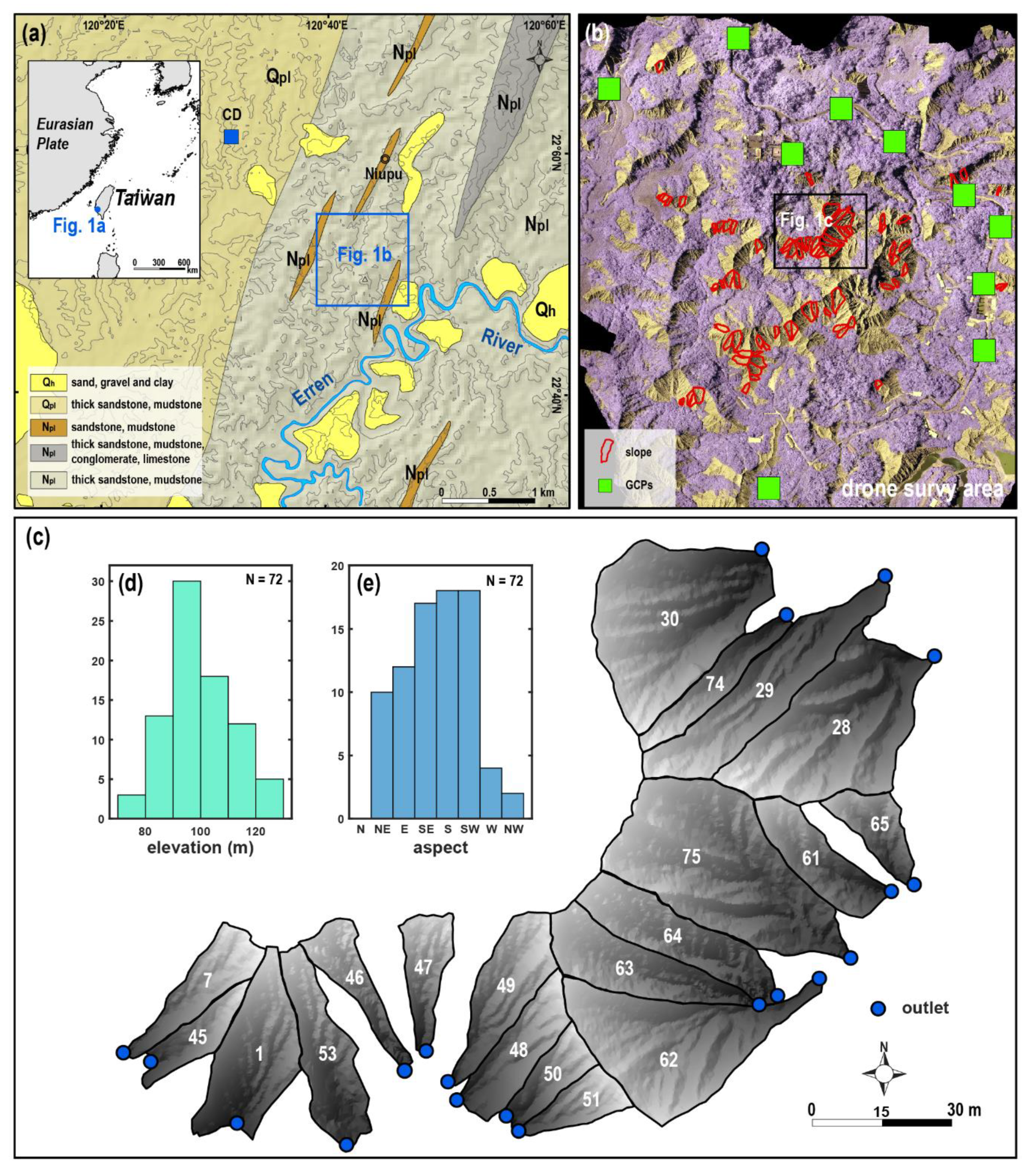
2.1. Study Area

Our study area comprises about 1 km² of badlands landscape in Tainan County, SW Taiwan (Figure 1a). This area hosts a military facility with high levels of security and, therefore, has undergone little intensive development in the past. Consequently, the area exhibits a natural landscape without extensive human disturbance and is, therefore highly suitable for a landscape-development study. It has a hot and wet tropical climate with major rainfalls from the seasonal monsoon and typhoons. The rainy season is between May and October and accounts on average for 89% of the total annual rainfall (2118 mm). The peak is in August with >400 mm of monthly rainfall on average. The average monthly rainfall is typically <40 mm from November to April.

The stratigraphy of the study area is dominated by clay and sandstone, which are prone to erosion caused by rainfall. As rainfall infiltrates the mudstone, the ionic bond link is destroyed and then releases strain energy, causing slaking. Illite (30.54%) and chlorite (28.70%) are the main minerals in the mudstone [5]. There is also a large proportion of soluble salt, which is easily dissolved by rainfall to form sodium ions. The sodium ions make soil particles disperse easily and result in slaking of the mudstone. After a long dry period, the mudstone surface shrinks and then forms cracks and crusts, 8–10 cm thick on the weathered surface layer and the cracks are preferential routes for infiltration. Plus, the alternate climate makes the annual erosional cycle in the the badland hillslope.

The typical badlands landscape is composed of steep slopes, dense rills, and gullies, as well as pipes or tunnels. Several studies have focused on the slope evolution of the mudstone areas in Taiwan. Yen [40] mentioned that the homogeneous lithology controlling the gradient tends to form hillslopes of 40–50° during the erosion process, followed by a parallel slope retreat. However, the longitudinal sections of the mudstone badlands slope are not completely linear, consisting of a steep slope in the upper part and a gentle slope in the lower part. The two steps in the slope indicate that the badlands slope evolution is simultaneously driven by gravity and water erosion. This implies that it is the external force, rather than tectonic movement, that mainly controls the form of the hillslope [40]. Yen and Chen [41] developed the landscape evolution of the mudstone badlands slope—drainage density, roughness, and local slope gradient would increase in the young state and decline the relief by climatic erosion and then eventually reach stabilization.

2.2. DEMs Created from UAV Surveys

UAV surveys were conducted between July and August of 2017. The dates of the acquisition were chosen according to the weather conditions. The two consequent typhoons (July 29–August 01), Nesat and Haitang, packed 579 mm of rainfall with the maximum rainfall intensity of 74 mm/h likely causing severe erosion in the mudstone areas. We conducted UAV surveys to collect surface near-infrared (NIR) images for DEM generation and ortho-rectification with a Canon s110 camera and an eBee Classic drone [43]. Detailed information on this equipment is provided in

Table 1. Information on the UAV surveys and resulting DEMs.

Date	Rainfall in This Period (mm)	Number of Images Obtained	Flight Height (m)	GSD (cm/pixel)	RMS * of Horizontal Errors (m)	RMS of Vertical Errors (m)	Point Cloud Density (pts/m2)
2017/07/01	748.1	111	330	11	0.01 ± 0.01	0.03 ± 0.04	159
2017/08/04		124	320	11	0.01 ± 0.02	0.04 ± 0.03	145

* RMS: root-mean-square.

.

In order to achieve a high survey accuracy, we installed 11 ground control points (GCPs) across the 1 km² surveying area (Figure 1b) and conducted high precision GCP surveys using a Leica RX1250XC differential GPS to obtain their coordinates. The GCPs were made of iron nails with a 5 mm diameter surrounded by aerial photogrammetric targets. All GCPs were positioned on solid sites, such as paved roads or bridges, to ensure stable anchoring for the survey. The coordinates of each GCP were measured over a period of more than 15 min using the real-time kinematic (RTK)-GPS system. The average flight altitude was 325 m and the average flight time to cover the entire study area was about 30 min. The resulting ortho-rectified images have a ground sample distance (GSD) of 11 cm. The data were transformed into 3D-models of the study area using the Acute 3D software (Bentley Systems).

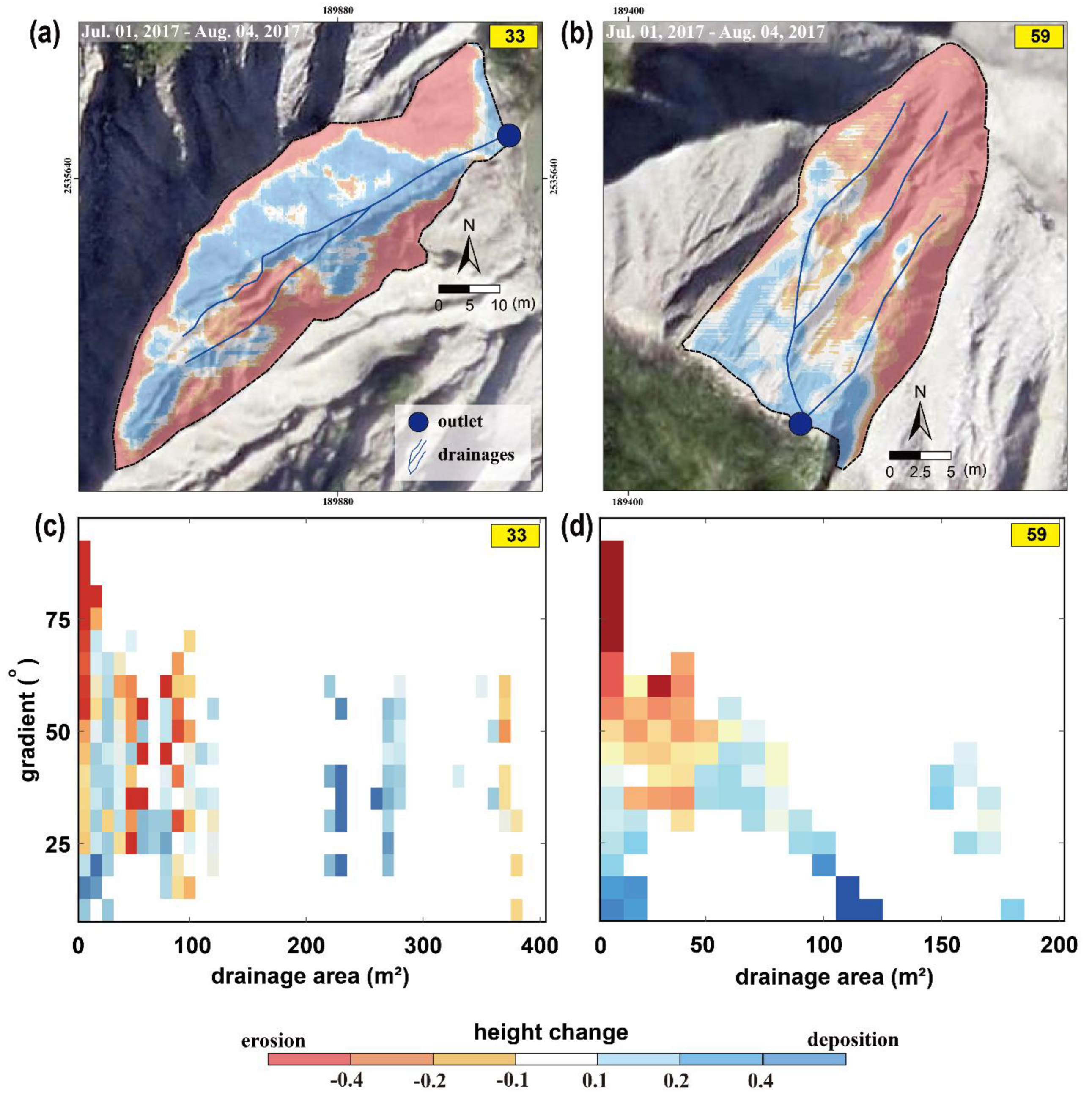
2.3. DEM of Difference (DoD)

DoD is the difference between two DEMs of the same area but acquired at two different times [44]. It reveals the geomorphic change and provides insight into the relationship between process and form. It can also be used to assess the simulation of numerical morphodynamic models. In this study, we constructed a DEM of each UAV survey and then obtained the DoD accordingly.

Wheaton et al. [44] and Williams [45] proposed that the DEM elevation value is likely to contain a vertical error component (or uncertainty). In DoDs, the combined errors are as follows:

$${\mathsf{\delta }\mathrm{U}}_{\mathrm{DoD}}=\sqrt{{\mathsf{\delta }\mathrm{Z}}_1^2+{\mathsf{\delta }\mathrm{Z}}_2^2}$$

(1)

where ${\mathsf{\delta }\mathrm{Z}}_1^{}$ and ${\mathsf{\delta }\mathrm{Z}}_2^{}$ are the errors associated with ${\mathrm{Z}}_1^{}$ and ${\mathrm{Z}}_2^{}$, respectively. We followed this method to calculate the error in our DoDs.

2.4. Parameter Extraction and Calculation of MSI

The geomorphological features of individual hillslopes were mapped manually using ArcGIS 10.5. The ortho-rectified UAV images were used to identify the hillslope divides and drainages. From the hillslope divides and drainages, we can calculate the plane tributary area (A_2D), slope length (L), circularity ratio (R_C), drainage frequency (F), drainage density (D), and drainage length (l). The slope inclination (P) is derived from the constructed DEM and we then calculate the reconstructed surface area (Ar) accordingly. The eroded volume (V) can reflect the amplitude of the transient topography in response to climate forces. The former is defined as the maximum vertical distance between drainage divide and valley bottom; the latter can be derived by creating a TIN surface capping the hillslope and subtracting the hillslope DEM from this surface, normalized by drainage area for comparison among hillslopes of different size (V/A_2D). The MSI is then calculated for the reconstructed slope of each hillslope [36]:

$$\mathrm{MSI}=\frac{{\mathrm{A}}_{\mathrm{r}}}{{\mathrm{A}}_{2\mathrm{D}}}\times \mathrm{L}\times {\mathrm{R}}_{\mathrm{C}}$$

(2)

Spearman’s correlation test was conducted to obtain the relationship between topographic indices calculated from the DEM and other data mentioned previously, and the MSI. The significance values of Spearman’s rank correlation coefficient (p-value) were set at 0.01 and 0.05, respectively.

3. Results

3.1. DoD Uncertainty Estimation

The DoD of the slopes studied between July 1st and August 4th, 2017 show a mean of 0.07 m and a standard deviation of ~0.01 m. The distribution of survey error in each grid is shown in Figure 2. As calculated, the uncertainty of DoD is ± 0.1 m. We, therefore, mark the change between ±0.1 m as uncertainty (error).

3.2. Morphometric Slope Index (MSI)

A total of 72 hillslopes were identified and mapped from the DEM obtained from the UAV data in the study area, as shown in Figure 1c. Overall, the elevation of the slopes range from 70 m to 130 m, and 42% of the 71 hillslopes are about 90–100 m in elevation (Figure 1d). In addition, 75% of the 71 hillslopes are S-facing (including SE, S, and SW) (Figure 1e). This implies that the effect of orographic precipitation and the difference of tectonic activity is negligible. The MSI of the 72 hillslopes is shown in

Table 2. Morphometric Slope Index (MSI) and morphometric features of different slopes. (F): drainage frequency (m⁻²); (D): drainage density (m⁻¹); (l): drainage length (m); (N): drainage number; (l/N): average drainage length (m); (L): slope length (m); (P): incision (°); (Rc): circularity ratio; (A_2D): plane tributary area (m²); (p): drainage basin perimeter; (Ar): reconstructed surface area (m²); (MSI): morphometric slope index (m); (V): erosion amount (m³); (V/A_2D): mean erosion depth (m).

Slope ID	F	D	L	N	l/N	L	P	Rc	V	V/A	MSI
1	0.03	0.16	110.59	19	5.82	52.90	48.92	0.50	1676.98	2.37	40.65
2	0.03	0.16	81.14	14	5.80	37.56	47.26	0.56	550.27	1.06	31.15
3	0.01	0.18	25.62	2	12.81	23.62	46.26	0.31	170.51	1.21	10.67
4	0.03	0.17	190.76	30	6.36	32.06	43.19	0.72	1239.45	1.14	31.55
5	0.03	0.17	158.71	24	6.61	34.58	44.67	0.65	2956.57	3.12	31.84
6	0.03	0.15	83.81	17	4.93	48.76	46.20	0.48	1386.21	2.43	33.48
7	0.03	0.21	84.87	11	7.72	39.83	45.25	0.41	97.39	0.24	23.41
8	0.03	0.18	77.78	13	5.98	39.66	48.76	0.55	657.67	1.55	32.80
9	0.02	0.15	112.01	17	6.59	43.68	46.81	0.61	2406.42	3.15	38.91
10	0.03	0.12	62.64	14	4.47	46.01	47.45	0.45	814.64	1.62	30.60
11	0.05	0.14	25.20	9	2.80	22.44	46.19	0.64	138.62	0.78	20.64
12	0.02	0.14	8.84	1	8.84	19.29	46.82	0.47	63.78	1.02	13.15
13	0.03	0.18	33.44	5	6.69	32.20	48.12	0.48	135.41	0.74	22.96
14	0.02	0.14	51.41	6	8.57	33.22	44.45	0.53	492.33	1.36	24.66
15	0.03	0.11	11.63	3	3.88	25.84	47.86	0.38	79.93	0.76	14.45
16	0.01	0.11	21.81	3	7.27	29.04	48.29	0.48	378.16	1.88	20.80
17	0.01	0.13	48.12	5	9.62	49.82	49.36	0.44	982.22	2.57	33.51
18	0.02	0.12	45.48	7	6.50	43.79	49.17	0.52	623.55	1.70	35.03
19	0.02	0.14	145.07	25	5.80	47.74	47.29	0.70	3767.89	3.53	49.36
20	0.03	0.16	17.44	3	5.81	23.54	50.36	0.59	92.44	0.86	21.86
21	0.02	0.15	166.73	19	8.78	56.04	47.00	0.57	3034.36	2.77	46.52
22	0.02	0.21	135.55	13	10.43	34.36	43.78	0.64	424.07	0.67	30.43
23	0.03	0.17	142.03	25	5.68	40.42	45.87	0.65	2219.02	2.60	37.47
24	0.02	0.14	54.26	9	6.03	26.13	46.14	0.69	498.76	1.32	26.04
25	0.03	0.15	86.27	15	5.75	34.33	46.07	0.61	764.64	1.29	29.97
26	0.03	0.14	48.35	10	4.84	32.94	46.37	0.58	871.05	2.50	27.88
27	0.03	0.35	42.67	4	10.67	27.45	47.69	0.27	124.88	1.03	11.14
28	0.02	0.13	185.82	27	6.88	49.60	47.25	0.57	592.74	0.41	41.52
30	0.02	0.16	246.35	27	9.12	47.92	47.01	0.74	3117.43	2.05	51.88
31	0.02	0.14	52.14	7	7.45	26.08	43.17	0.33	504.93	1.37	11.83
32	0.03	0.17	65.31	11	5.94	31.61	46.66	0.63	749.07	1.93	29.21
33	0.01	0.14	49.32	5	9.86	32.55	44.60	0.45	623.54	1.73	20.56
35	0.02	0.16	24.86	3	8.29	25.09	49.76	0.51	172.95	1.13	19.74
36	0.01	0.13	14.56	1	14.56	22.76	49.14	0.40	94.93	0.85	14.08
37	0.01	0.11	53.98	7	7.71	28.17	44.92	0.58	29.87	0.06	22.97
38	0.01	0.11	55.53	7	7.93	31.70	47.45	0.58	982.93	1.97	27.35
39	0.03	0.15	29.69	5	5.94	21.81	43.02	0.45	197.19	1.01	13.50
40	0.03	0.12	51.03	12	4.25	27.24	46.85	0.67	585.24	1.42	26.64
41	0.03	0.11	29.77	7	4.25	22.36	46.14	0.72	452.40	1.71	23.12
42	0.03	0.14	40.51	8	5.06	23.21	44.96	0.59	460.12	1.60	19.21
45	0.01	0.12	32.11	3	10.70	34.93	47.44	0.41	48.38	0.18	21.18
46	0.02	0.16	51.14	5	10.23	42.46	47.53	0.35	259.00	0.82	22.12
47	0.02	0.15	45.81	7	6.54	31.35	45.81	0.48	292.51	0.93	21.56
48	0.02	0.17	71.36	10	7.14	36.86	45.48	0.48	491.18	1.15	25.17
49	0.02	0.15	83.29	10	8.33	46.10	47.16	0.50	796.72	1.45	33.79
50	0.03	0.16	43.43	7	6.20	30.96	47.98	0.54	477.71	1.77	25.11
51	0.03	0.18	46.22	7	6.60	25.70	45.67	0.54	242.27	0.97	19.78
52	0.02	0.14	8.07	1	8.07	18.16	50.58	0.58	36.09	0.61	16.45
53	0.02	0.13	71.63	13	5.51	48.91	48.19	0.41	1043.70	1.87	30.08
54	0.02	0.22	72.11	6	12.02	40.03	48.32	0.45	572.62	1.76	26.79
55	0.02	0.14	36.87	5	7.37	40.07	51.19	0.51	356.61	1.33	32.89
56	0.03	0.17	93.62	16	5.85	45.51	45.40	0.39	975.78	1.79	25.40
57	0.02	0.18	100.47	11	9.13	47.02	46.57	0.44	1140.62	2.03	30.24
58	0.03	0.15	76.22	13	5.86	48.83	49.34	0.51	1053.05	2.03	38.21
59	0.04	0.31	52.90	6	8.82	25.83	43.91	0.32	222.24	1.32	11.40
60	0.02	0.12	16.80	3	5.60	26.39	47.72	0.46	92.38	0.68	17.95
61	0.02	0.10	46.50	9	5.17	36.71	47.97	0.54	747.03	1.62	29.83
63	0.03	0.12	79.11	17	4.65	60.27	49.47	0.42	1494.95	2.33	39.35
64	0.02	0.15	90.84	10	9.08	57.44	48.78	0.40	1131.70	1.93	35.18
65	0.02	0.11	31.39	5	6.28	28.05	48.25	0.56	383.65	1.35	23.69
66	0.02	0.11	32.20	7	4.60	32.27	45.99	0.49	383.88	1.27	22.73
67	0.02	0.12	187.65	29	6.47	71.91	51.26	0.57	6439.13	4.03	65.52
68	0.02	0.12	148.08	23	6.44	47.46	47.51	0.65	2607.65	2.13	45.72
69	0.01	0.17	16.38	1	16.38	19.18	43.67	0.39	38.12	0.40	10.28
70	0.02	0.14	19.89	3	6.63	26.61	47.42	0.41	181.94	1.27	16.21
71	0.01	0.13	19.95	1	19.95	24.49	47.59	0.40	217.80	1.41	14.59
72	0.03	0.17	54.81	9	6.09	38.57	51.36	0.57	632.27	1.98	35.43
73	0.01	0.12	24.74	3	8.25	36.54	52.63	0.52	559.03	2.63	31.58
75	0.02	0.12	216.37	43	5.03	59.95	48.13	0.64	6840.12	3.92	57.40
76	0.03	0.29	56.08	6	9.35	31.39	43.90	0.31	87.66	0.45	13.51
79	0.01	0.10	21.46	3	7.15	21.36	45.02	0.60	229.54	1.11	18.12
81	0.01	0.09	43.40	7	6.20	33.43	47.02	0.74	1361.89	2.87	36.16

.

The relationship between MSI and morphometric features is shown in

Table 3. Pearson’s correlation matrix of MSI and morphometric features.

	F	D	l	N	l/N	L	P	Rc	V	V/A2D
F	1
D	0.41 **	1
l	0.24 *	0.29 *	1
N	0.40 **	0.12	0.92 **	1
l/N	−0.61 **	0.34 **	−0.10	−0.43 **	1
L	0.01	0.01	0.78 **	0.71 **	0.10	1
P	−0.21	−0.28 *	−0.15	−0.14	−0.02	0.32 **	1
Rc	0.10	−0.21	0.32 **	0.49 **	−0.41 **	0.06	−0.08	1
V	0.10	−0.07	0.79 **	0.83 **	−0.30 *	0.77 **	0.11	0.23	1
V/A2D	0.02	−0.18	0.49 **	0.53 **	−0.26 *	0.59 **	0.27 *	0.03	0.87 **	1
MSI	0.03	−0.12	0.77 **	0.79 **	−0.27 *	0.86 **	0.32 **	0.41 **	0.87 **	0.70 **

** Significant correlation at the 0.01 level. * Significant correlation at the 0.05 level.

. MSI has a strong positive correlation with total drainage length (R² = 0.77), total number of furrows (R² = 0.79), plane length (R² = 0.86), eroded volume (R² = 0.87), and mean eroded depth (R² = 0.70). In addition, it also has no correlation with inclination (R² = 0.32) and circularity ratio (R² = 0.41). In contrast, it has no correlation with drainage density (R² = −0.12) and mean drainage length (R² = −0.27).

3.3. Distribution of Hillslope Erosion

Over the surveyed periods, about 68% of the study area was affected by erosion. We measured 31 cm of average erosion depth during the typhoon. The two selected badlands hillslopes represent the erosion pattern (Figure 3). Overall, Hillslope 33 exhibited the largest observed erosion rate, located on the steepest hillslopes and at sites with drainage areas under 100 m². In addition, erosion and deposition occurred simultaneously in drainage areas under 100 m² s. Drainage areas between 200 m² and 300 m² predominantly exhibited a deposition of 0.4 m, and these are the areas where the main gully is distributed (Figure 3c). Furthermore, erosion and deposition occurred in drainage areas over 300 m² but resulted in a change of only ± 0.1 m. On Hillslope 59, the observed erosion was also located on the steepest hillslopes with gradients greater than 40°, and at sites with drainage areas under 50 m² (Figure 3d). In contrast, deposition occurred in relatively gentle areas with slope gradients under 50°, and the deposition rate increased with decreases in slope gradient.

4. Discussion

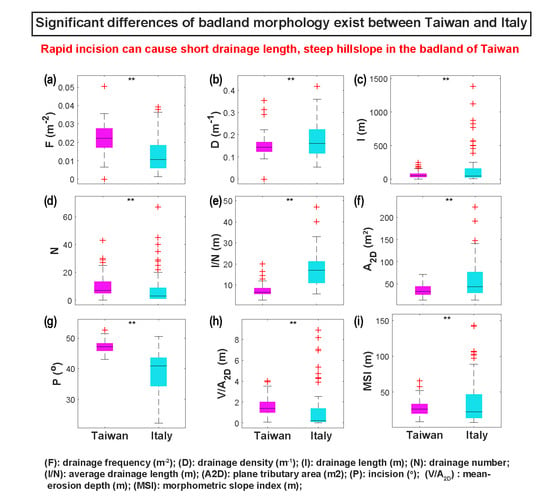
4.1. The Effect of Rapid Incision on Morphology of Hillslopes in Badlands

In order to isolate the topographic effects of different climatic forcing it is essential to understand how landscapes work on badlands evolution. The calculated MSI in this study was compared to the results of Buccolini et al. [36] (Figure 4), who documented 65 morphological features of hillslopes and MSI in the central Sicily. Badlands in Taiwan have lower drainage length and drainage density than those in Italy, which may imply that the relatively small hillslope area controls the drainage network development. The badlands in the study area are caused by incision into weakly resistant mudrocks of the river terrace [46], and the formation of mudstone badlands is mainly controlled by climatic erosion, i.e., high rainfall events brought by either typhoons or summer monsoons. The strong climatic erosion also steepens the hillslope to an average hillslope inclination of 47.1°, which is 8.3° higher than that of the badlands in Sicily, Italy. Additionally, the origin of the river terrace is ascribed to strong uplift combined with a storm-induced incision in unconsolidated mudstone since 2000 YBP [46]. Such a young badlands landscape may explain why the morphology of badlands landscapes in Taiwan is relatively short, small, and steep. However, the annual precipitation in the Taiwan badlands is three times higher than in those of Italy, which may still cause strong erosional feedback, i.e., rills and gullies. Thus, badlands in Taiwan have a higher drainage frequency and a greater number of furrows.

4.2. Distinct Erosion Patterns in the Badlands Landscapes of Taiwan

In Taiwan, the higher mean eroded depth (Figure 4h) suggests that more sediment can be produced from the tiny hillslopes, which has low drainage density. To our knowledge, gully erosion in Taiwan is a dominant contributor to sediment production during the rainy season. However, no correlation between drainage density and mean eroded depth (R² = −0.18) are consistent with the results from Italy, and this may suggest that the drainages in Taiwan could play the specific role of shredding the landscape, instead of transporting eroded material, such as gully erosion (Figure 5a) and, therefore, high drainage frequency likely cause more free-surface, making hillslopes more prone to erosion. Moreover, no correlation between drainage density and mean eroded depth (R² = −0.26) can explain why the relatively short drainage length in Taiwan is not the main contribution to soil loss. Besides, the observed difference of mean eroded depth, which reflects slope inclination (Figure 5c), may suggest that the erosional pattern is mainly due to gravitational mass wasting, which preferentially occurred during high-intensity rainfall events [47,48,49,50,51]. In addition, the mean circularity ratio is 0.52 in Taiwan, which suggests that the shape of the badlands is not affected by the evolution of a single gully but expands through many short drainage systems. Thus, the mean erosion depth is not influenced by the circularity ratio, which may also suggest that hydrological erosion is not the main erosional process.

During the study period, the total rainfall was 748.1 mm over 35 days (typhoons brought 579 mm of rainfall, with a maximum intensity of 74 mm/h). The high rainfall intensity causes severe erosion of the steepest areas in the badlands slopes. The eroded material was then transported downwards and deposited in the lower part of the gully or downstream area (Figure 3). The observed erosion pattern is consistent with the argument that gravitational mass wasting dominates the steep areas of the slope during storm events.

4.3. Benefitting from the UAV-Driven High-Resolution Topography in Application of MSI

Traditionally, the investigation of hillslope erosion, i.e., landslides or gully erosion, has been conducted directly through on-site human surveys or through satellite imagery technology (e.g., [52,53,54]). The results of this study demonstrate the practicality and feasibility of using UAV data for topographical analysis of landscape change. A combination of UAV and RTK-GPS surveys can facilitate the efficient acquisition of high-precision and accurate information about slope erosion. This particularly benefits the construction of high-resolution DEMs and DoDs for studying erosion patterns and volumes. The detailed topographic data also further extends the understanding of erosional processes, which is essential to understanding the response of a landscape to climatic forces. Our findings suggest that high-resolution topographic UAV surveys may guide further investigations in other badland areas or active-hillslope erosion regions across climatic zones. This may provide opportunities for clarifying the reaction of morphometric features to different environments. For further application of MSI, two related issues need to be considered. Firstly, while slope length is a function of MSI, the scale of hillslopes can range from tens to hundreds of meters. Therefore, the normalized slope length should always be used. Secondly, MSI is representative of hydrological erosion but is not suitable for landslide-dominated areas. Thus, we suggest that using UAV-driven DEMs to construct the DoD is beneficial for identifying erosion distribution, especially in areas of high rainfall intensity.

5. Conclusions

Through a morphometric analysis of UAV-acquired DEMs and DoDs, we have reached the following conclusions. First, by conducting UAV surveys, we were able to quantify the landform change to centimeter-scale accuracy across 72 badlands hillslopes and construct high-resolution DEMs and DoDs. These provide reliable data constraint on the relationship between hillslope-morphology and erosion and will benefit the monitoring of land surface change as a result of exogenic forces.

The topographic effects of the climatic difference are important to reveal the mechanism of landscape evolution. Our observations indicate that badlands hillslopes in Taiwan are relatively short, small, and steep compared with those of Italy. Because the annual precipitation of over 2 m causes strong incision, the mudstone badlands in Taiwan are characterized by higher drainage frequency and more furrows. Thus, we suggest that MSI can be used in the badlands areas of Taiwan. Our findings suggest that MSI has a strong positive correlation with erosion, which is consistent with results from Italy. However, the mean eroded depth shows no correlation with mean drainage length and a positive correlation with inclination, suggesting that the erosion pattern is due to gravitational mass wasting, rather than hydrological erosion.

MSI combined with UAV-driven DEMs, provides a relatively convenient and rapid method for assessing the severity of soil loss and evaluating landscape maturity. We highlight the unique cross-climate zone comparative study offered by badlands landscapes, with differential rainfall patterns, using simple survey techniques and morphometric slope index. The results of this study also suggest that UAV techniques are able to provide quantitative evidence for hillslope morphological analysis, and through simple morphological indicators, we can achieve comparative studies in different climate zones.

References

1. Valentin, C.; Poesen, J.; Li, Y. Gully erosion: Impacts, factors and control. Catena 2005, 63, 132–153. [Google Scholar] [CrossRef]
2. Gomez, B.; Banbury, K.; Marden, M.; Trustrum, N.A.; Peacock, D.H.; Hoskin, P.J. Gully erosion and sediment production: Te Weraroa Stream, New Zealand. Water Resour. Res. 2003, 39. [Google Scholar] [CrossRef] [Green Version]
3. Castaldi, F.; Chiocchini, U. Effects of land use changes on badland erosion in clayey drainage basins, Radicofani, Central Italy. Geomorphology 2012, 169, 98–108. [Google Scholar] [CrossRef]
4. Mongil-Manso, J.; Navarro-Hevia, J.; Díaz-Gutiérrez, V.; Cruz-Alonso, V.; Ramos-Díez, I. Badlands forest restoration in Central Spain after 50 years under a Mediterranean-continental climate. Ecol. Eng. 2016, 97, 313–326. [Google Scholar] [CrossRef]
5. Lee, D.-H.; Lin, H.-M.; Wu, J.-H. The Basic Properties Of Mudstone Slope In Southwestern Taiwan. J. GeoEng. 2007, 2, 15. [Google Scholar]
6. Higuchi, K.; Chigira, M.; Lee, D.-H. High rates of erosion and rapid weathering in a Plio-Pleistocene mudstone badland, Taiwan. Catena 2013, 106, 68–82. [Google Scholar] [CrossRef]
7. Kao, S.-J.I.; Milliman, J. Water and Sediment Discharge from Small Mountainous Rivers, Taiwan: The Roles of Lithology, Episodic Events, and Human Activities. J. Geol. 2008, 116, 431–448. [Google Scholar] [CrossRef] [Green Version]
8. Benito, G.; Gutie’rrez, M.; Sancho, C. Erosion rates in badland areas of the central Ebro Basin (NE-Spain). Catena 1992, 19, 269–286. [Google Scholar] [CrossRef]
9. Clarke, M.L.; Rendell, H.M. Process–form relationships in Southern Italian badlands: Erosion rates and implications for landform evolution. Earth Surf. Process. Landf. 2006, 31, 15–29. [Google Scholar] [CrossRef]
10. Sirvent, J.; Desir, G.; Gutiérrez, M.; Sancho, C.; Benito, G. Erosion rates in badland areas recorded by collectors, erosion pins and profilometer techniques (Ebro Basin, NE-Spain). Geomorphology 1997, 18, 61–75. [Google Scholar] [CrossRef]
11. Neugirg, F.; Stark, M.; Kaiser, A.; Vlacilova, M.; Della Seta, M.; Vergari, F.; Schmidt, J.; Becht, M.; Haas, F. Erosion processes in calanchi in the Upper Orcia Valley, Southern Tuscany, Italy based on multitemporal high-resolution terrestrial LiDAR and UAV surveys. Geomorphology 2016, 269, 8–22. [Google Scholar] [CrossRef]
12. Eltner, A.; Baumgart, P.; Maas, H.-G.; Faust, D. Multi-temporal UAV data for automatic measurement of rill and interrill erosion on loess soil. Earth Surf. Process. Landf. 2015, 40, 741–755. [Google Scholar] [CrossRef]
13. Fonstad, M.; Dietrich, J.; Courville, B.; Jensen, J.; Carbonneau, P. Topographic Structure from Motion: A new development in photogrammetric measurement. Earth Surf. Process. Landf. 2013, 38, 421–430. [Google Scholar] [CrossRef] [Green Version]
14. Hugenholtz, C.H.; Whitehead, K.; Brown, O.W.; Barchyn, T.E.; Moorman, B.J.; LeClair, A.; Riddell, K.; Hamilton, T. Geomorphological mapping with a small unmanned aircraft system (sUAS): Feature detection and accuracy assessment of a photogrammetrically-derived digital terrain model. Geomorphology 2013, 194, 16–24. [Google Scholar] [CrossRef] [Green Version]
15. Bianchini, S.; Del Soldato, M.; Solari, L.; Nolesini, T.; Pratesi, F.; Moretti, S. Badland susceptibility assessment in Volterra municipality (Tuscany, Italy) by means of GIS and statistical analysis. Environ. Earth Sci. 2016, 75, 889. [Google Scholar] [CrossRef]
16. Del Soldato, M.; Riquelme, A.; Tomás, R.; De Vita, P.; Moretti, S. Application of structure from motion photogrammetry to multi-temporal geomorphological analyses: Case studies from Italy and Spain. Geogr. Fis. Din. Quat. 2018, 41, 97–102. [Google Scholar] [CrossRef]
17. Afana, A.; Sole-Benet, A.; Perezc, J.L. Determination of Soil Erosion Using Laser Scanners. In Proceedings of the 19th World Congress of Soil Science, Soil Solutions for a Changing World, Brisbane, Australia, 1–6 August 2010; pp. 39–42. [Google Scholar]
18. Milan, D.; Heritage, G.; Hetherington, D. Application of a 3D laser scanner in the assessment of erosion and deposition volumes in a proglacial river. Earth Surf. Process. Landf. 2007, 32, 1657–1674. [Google Scholar] [CrossRef]
19. Tarolli, P. High-resolution topography for understanding Earth surface processes: Opportunities and challenges. Geomorphology 2014, 216, 295–312. [Google Scholar] [CrossRef]
20. Cheng, Y.-C.; Yang, C.-J.; Lin, J.-C. Application for Terrestrial LiDAR on Mudstone Erosion Caused by Typhoons. Remote Sens. 2019, 11, 2425. [Google Scholar] [CrossRef] [Green Version]
21. Westoby, M.J.; Brasington, J.; Glasser, N.F.; Hambrey, M.J.; Reynolds, J.M. ‘Structure-from-Motion’ photogrammetry: A low-cost, effective tool for geoscience applications. Geomorphology 2012, 179, 300–314. [Google Scholar] [CrossRef] [Green Version]
22. Adams, S.; Friedland, C. A Survey of Unmanned Aerial Vehicle (UAV) Usage for Imagery Collection in Disaster Research and Management. In Proceedings of the 9th International Conference on Geoinformation for Disaster Management (Gi4DM), Hanoi, Vietnam, 9–11 December 2013. [Google Scholar]
23. Pajares, G. Overview and Current Status of Remote Sensing Applications Based on Unmanned Aerial Vehicles (UAVs). Photogramm. Eng. Remote Sens. 2015, 81, 281–329. [Google Scholar] [CrossRef] [Green Version]
24. Gomez, C.; Purdie, H. UAV-based Photogrammetry and Geocomputing for Hazards and Disaster Risk Monitoring—A Review. Geoenviron. Disasters 2016, 3, 23. [Google Scholar] [CrossRef] [Green Version]
25. Angster, S.; Wesnousky, S.; Huang, W.l.; Kent, G.; Nakata, T.; Goto, H. Application of UAV Photography to Refining the Slip Rate on the Pyramid Lake Fault Zone, Nevada. Bull. Seismol. Soc. Am. 2016, 106, 785–798. [Google Scholar] [CrossRef] [Green Version]
26. Bi, H.; Zheng, W.; Ren, Z.; Zeng, J.; Yu, J. Using an unmanned aerial vehicle for topography mapping of the fault zone based on structure from motion photogrammetry. Int. J. Remote Sens. 2017, 38, 2495–2510. [Google Scholar] [CrossRef]
27. Shi, X.; Weldon, R.; Liu-Zeng, J.; Wang, Y.; Weldon, E.; Sieh, K.; Li, Z.; Zhang, J.; Yao, W.; Li, Z. Limit on slip rate and timing of recent seismic ground-ruptures on the Jinghong fault, SE of the eastern Himalayan syntaxis. Tectonophysics 2018, 734, 148–166. [Google Scholar] [CrossRef]
28. Tamminga, A.; Hugenholtz, C.; Eaton, B.; Lapointe, M. Hyperspatial Remote Sensing of Channel Reach Morphology and Hydraulic Fish Habitat Using an Unmanned Aerial Vehicle (UAV): A First Assessment in the Context of River Research and Management. River Res. Appl. 2015, 31, 379–391. [Google Scholar] [CrossRef]
29. Cook, K.L. An evaluation of the effectiveness of low-cost UAVs and structure from motion for geomorphic change detection. Geomorphology 2017, 278, 195–208. [Google Scholar] [CrossRef]
30. Langhammer, J.; Vacková, T. Detection and Mapping of the Geomorphic Effects of Flooding Using UAV Photogrammetry. Pure Appl. Geophys. 2018, 175, 3223–3245. [Google Scholar] [CrossRef]
31. Niethammer, U.; James, M.R.; Rothmund, S.; Travelletti, J.; Joswig, M. UAV-based remote sensing of the Super-Sauze landslide: Evaluation and results. Eng. Geol. 2012, 128, 2–11. [Google Scholar] [CrossRef]
32. Lucieer, A.; Jong, S.M.d.; Turner, D. Mapping landslide displacements using Structure from Motion (SfM) and image correlation of multi-temporal UAV photography. Prog. Phys. Geogr. Earth Environ. 2014, 38, 97–116. [Google Scholar] [CrossRef]
33. Turner, D.; Lucieer, A.; De Jong, S.M. Time Series Analysis of Landslide Dynamics Using an Unmanned Aerial Vehicle (UAV). Remote Sens. 2015, 7, 1736–1757. [Google Scholar] [CrossRef] [Green Version]
34. Saito, H.; Uchiyama, S.; Hayakawa, Y.S.; Obanawa, H. Landslides triggered by an earthquake and heavy rainfalls at Aso volcano, Japan, detected by UAS and SfM-MVS photogrammetry. Prog. Earth Planet. Sci. 2018, 5, 15. [Google Scholar] [CrossRef]
35. Rossi, G.; Tanteri, L.; Tofani, V.; Vannocci, P.; Moretti, S.; Casagli, N. Multitemporal UAV surveys for landslide mapping and characterization. Landslides 2018, 15, 1045–1052. [Google Scholar] [CrossRef] [Green Version]
36. Buccolini, M.; Coco, L.; Cappadonia, C.; Rotigliano, E. Relationships between a new slope morphometric index and calanchi erosion in northern Sicily, Italy. Geomorphology 2012, 149, 41–48. [Google Scholar] [CrossRef]
37. Buccolini, M.; Coco, L. The role of the hillside in determining the morphometric characteristics of “calanchi”: The example of Adriatic central Italy. Geomorphology 2010, 123, 200–210. [Google Scholar] [CrossRef]
38. Buccolini, M.; Coco, L. MSI (morphometric slope index) for analyzing activation and evolution of calanchi in Italy. Geomorphology 2013, 191, 142–149. [Google Scholar] [CrossRef]
39. Buccolini, M.; Materazzi, M.; Aringoli, D.; Gentili, B.; Pambianchi, G.; Scarciglia, F. Late Quaternary catchment evolution and erosion rates in the Tyrrhenian side of central Italy. Geomorphology 2014, 204, 21–30. [Google Scholar] [CrossRef]
40. Yen, F.-S. Study on stability process of natural rock slope in mudstone slope land in southwestern Taiwan. Natl. Sci. Counc. Exec. Yuan Disaster Prev. Sci. Technol. Res. Rep. 1992, 80, 1–33. [Google Scholar]
41. Yen, F.-S.; Chen, J.-K. The relationships between the morphology and the weathering-erosion behavior of mudstone slopes in the southwestern Taiwan. Natl. Sci. Counc. Exec. Yuan Disaster Prev. Sci. Technol. Res. Rep. 1989, 78, 1–36. [Google Scholar]
42. Central Geological Survey, Ministry of Economic Affairs (MOEA). Geologic Map of Taiwan: Qishan Sheet, Scale 1:50,000; Central Geological Survey: New Taipei City, Taiwan, 2013.
43. SenseFly. eBee Classic Specification. Available online: https://www.sensefly.com/drone/ebee-mapping-drone/ (accessed on 17 November 2019).
44. Wheaton, J.M.; Brasington, J.; Darby, S.E.; Sear, D.A. Accounting for uncertainty in DEMs from repeat topographic surveys: Improved sediment budgets. Earth Surf. Process. Landf. 2010, 35, 136–156. [Google Scholar] [CrossRef]
45. Williams, R.D. DEMs of Difference. In Geomorphological Techniques (Online Edition); Cook, S.J., Clarke, L.E., Nield, J.M., Eds.; British Society for Geomorphology: London, UK, 2012; pp. 1–17. [Google Scholar]
46. Hsieh, M.-L.; Knuepfer, P.L.K. Middle–late Holocene river terraces in the Erhjen River Basin, southwestern Taiwan—Implications of river response to climate change and active tectonic uplift. Geomorphology 2001, 38, 337–372. [Google Scholar] [CrossRef]
47. Seta, D.M.; Monte, M.; Fredi, P.; Lupia Palmieri, E. Gully erosion in central Italy: Denudation rate estimation and morphoevolution of Calanchi and Biancane badlands. In Proceedings of the IV International Symposium on Gully Erosion, Pamplona, Spain, 17–19 September 2007; Public University of Navarra: Pamplona, Spain, 2007. [Google Scholar]
48. Sirio, C.; Galiano, M.; Roma, M.; Salvatore, M.C. Morphological analysis and erosion rate evaluation in badlands of Radicofani area (Southern Tuscany—Italy). Catena 2008, 74, 87–97. [Google Scholar] [CrossRef]
49. Densmore, A.L.; Hovius, N. Topographic fingerprints of bedrock landslides. Geology 2000, 28, 371–374. [Google Scholar] [CrossRef]
50. Meunier, P.; Hovius, N.; Haines, J. Topographic site effects and the location of earthquake induced landslides. Earth Planet. Sci. Lett. 2008, 275, 221–232. [Google Scholar] [CrossRef]
51. Huang, J.-C.; Milliman, J.D.; Lee, T.-Y.; Chen, Y.-C.; Lee, J.-F.; Liu, C.-C.; Lin, J.-C.; Kao, S.-J. Terrain attributes of earthquake- and rainstorm-induced landslides in orogenic mountain Belt, Taiwan. Earth Surf. Process. Landf. 2017, 42, 1549–1559. [Google Scholar] [CrossRef]
52. Kääb, A. Monitoring high-mountain terrain deformation from repeated air- and spaceborne optical data: Examples using digital aerial imagery and ASTER data. ISPRS J. Photogramm. Remote Sens. 2002, 57, 39–52. [Google Scholar] [CrossRef]
53. Liu, J.G.; Mason, P.; Clerici, N.; Chen, S.; Davis, A.; Miao, F.; Deng, H.; Liang, L. Landslide hazard assessment in the Three Gorges area of the Yangtze River using ASTER imagery: Zigui-Badong. Geomorphology 2004, 61, 171–187. [Google Scholar] [CrossRef]
54. Nichol, J.E.; Shaker, A.; Wong, M.-S. Application of high-resolution stereo satellite images to detailed landslide hazard assessment. Geomorphology 2006, 76, 68–75. [Google Scholar] [CrossRef]
Figure 1. Location and geological background of the study site. (a) The geological map of the study area [42](Niupu, Tainan City). (b) The NIR image derived from the UAV survey. The red areas denote selected slopes in this study and green squares denote ground control points (GCPs) for the UAV survey. (c) Examples of slope unit and (d), (e) denote centroid elevation and aspect of all slopes, respectively.
Remotesensing 11 03051 g001
Figure 2. Probability density of the survey error. The gray area denotes the binned probability of the survey error, the box plot displays an error distribution, and the red solid line denotes the fitting curve of the Gaussian distribution.
Remotesensing 11 03051 g002
Figure 3. Distribution of height change obtained from the DEMs by the UAV survey between July 01, 2017 and August 04, 2017.
Remotesensing 11 03051 g003
Figure 4. Boxplots showing that significant differences (p-value < 0.01) exist between Taiwan and Italy in terms of drainage frequency, drainage density, total drainage network length, total number of furrows in the drainage unit, mean drainage network length, plane length, inclination, mean eroded depth, and MSI.
Remotesensing 11 03051 g004
Figure 5. The relationship between mean eroded depth and morphometric features. Red solid dots and red R-square represent the dataset of this study; Blue solid dots and blue R-square represent the dataset of Buccolini et al., 2012.
Remotesensing 11 03051 g005