Cloud Detection from FY-4A’s Geostationary Interferometric Infrared Sounder Using Machine Learning Approaches

Abstract

FengYun-4A (FY-4A)’s Geostationary Interferometric Infrared Sounder (GIIRS) is the first hyperspectral infrared sounder on board a geostationary satellite, enabling the collection of infrared detection data with high temporal and spectral resolution. As clouds have complex spectral characteristics, and the retrieval of atmospheric profiles incorporating clouds is a significant problem, it is often necessary to undertake cloud detection before further processing procedures for cloud pixels when infrared hyperspectral data is entered into assimilation system. In this study, we proposed machine-learning-based cloud detection models using two kinds of GIIRS channel observation sets (689 channels and 38 channels) as features. Due to differences in surface cover and meteorological elements between land and sea, we chose logistic regression (lr) model for the land and extremely randomized tree (et) model for the sea respectively. Six hundred and eighty-nine channels models produced slightly higher performance (Heidke skill score (HSS) of 0.780 and false alarm rate (FAR) of 16.6% on land, HSS of 0.945 and FAR of 4.7% at sea) than 38 channels models (HSSof 0.741 and FAR of 17.7% on land, HSS of 0.912 and FAR of 7.1% at sea). By comparing visualized cloud detection results with the Himawari-8 Advanced Himawari Imager (AHI) cloud images, the proposed method has a good ability to identify clouds under circumstances such as typhoons, snow covered land, and bright broken clouds. In addition, compared with the collocated Advanced Geosynchronous Radiation Imager (AGRI)-GIIRS cloud detection method, the machine learning cloud detection method has a significant advantage in time cost. This method is not effective for the detection of partially cloudy GIIRS’s field of views, and there are limitations in the scope of spatial application.

1. Introduction

Improvements in forecasting weather patterns have advanced due to the assimilation of data from hyperspectral infrared (HIR) sounders on meteorological satellites into operational numerical weather prediction systems. These sounders include the Atmospheric Infrared Sounder (AIRS) on board the National Aeronautics and Space Administration (NASA) Earth Observing System (EOS) Aqua platform [1,2], the Infrared Atmospheric Sounding Interferometer (IASI) on board the European Meteorological Operational (MetOp) satellites [2,3], and the Cross-Track Infrared Sounder (CrIS) on board the Suomi National Polar-Orbiting Partnership [2,4]. In order to reliably predict high-impact weather events, such as local severe storms, it is important that atmospheric temperature and moisture information with a high temporal/spatial resolution, two key parameters in regional Numerical Weather Prediction (NWP) models are accurately obtained. Compared with low earth orbit sounders, a HIR sounder from a GEostationary Orbit (GEO) has a higher temporal resolution and local continuous detection capability, providing tracking information with high temporal and vertical resolution in local rapidly developing weather processes [5].

A new generation of Chinese geostationary meteorological satellites was introduced with the launch of the first FengYun-4A (FY-4A) on 11th December 2016, equipped with four payloads: Geostationary Interferometric Infrared Sounder (GIIRS), Advanced Geosynchronous Radiation Imager (AGRI), Lightning Mapping Imager (LMI), and the Space Environment Package (SEP) [6,7]. FY-4A’s GIIRS is the first high spectral resolution advanced infrared sounder on board a geostationary weather satellite, aiming to obtain rapidly changing water vapor and temperature structures and contents of trace gases in China and the surrounding areas. Information from the GIIRS provides three-dimensional dynamic and thermodynamic information required to improve nowcasting and NWP services, important for estimating diurnal variations of trace gases that support forecasting air quality and monitoring of atmospheric minor constituents [6,7].

For infrared spectra, liquid water and ice crystals in clouds result in satellite sensors not detecting atmospheric or ground radiation below the upper cloud layer [8]. In addition, it is currently difficult for radiation transfer observation operators to accurately simulate radiation effects of clouds, and the weather forecast model is not perfect, resulting in difficulties in accurately providing cloud water profile information [9]. As the spatial resolution of HIR is low, and there are very few completely cloudless pixels in all Field of Views (FOVs)s (usually only about 10%) in instruments with a spatial resolution of 10 km [10]. Although existing hyperspectral sounders usually produce high-spectral-resolution, due to technical constraints they produce low-spatial resolution data. Therefore, in actual quantitative applications of infrared hyperspectral data, data contaminated by clouds must be eliminated or alternative pre-processing of cloud pixels must be undertaken, such as cloud clearing [11] or clear channel detection [12]. The process of judging whether clouds exist in a FOV is called cloud detection, and this is the first step before dealing with cloud contaminated FOVs, being an important step in the use of HIR data. GIIRS data also needs to go through cloud detection when entering the assimilation system.

Currently, some multi-channels threshold methods are proposed on the basis of cloud physical characteristics as clouds have higher reflectivity relative to land/sea surfaces in the visible and near infrared bands, and lower temperatures in infrared bands, for example the International Satellite Cloud Climatology Project (ISCCP) method [13,14], the AVHRR (Advanced Very High Resolution Radiometer) Processing Scheme Over Clouds, Land and Ocean (APOLLO) method [15], the Clouds from AVHRR (CLAVR) method [16], the CO2 slicing method [17], and the Moderate Resolution Imaging Spectroradiometer (MODIS) cloud detection method [18,19]. Due to its solid physical background, the multi-band threshold method effectively provides the required resolution and spectral range. However, this method cannot be used by HIR sounders for spectral bands and spatial resolution limitations.

At present, the cloud detection method assisted with imagers for HIR sounders is widely used. AIRS cloud detection is objectively determined by spatially matching 1 km MODIS cloud detection products that fall into each AIRS FOV [20]. Eressmaa [21] used three criteria to evaluate the AVHRR FOVs that falls in the IASI FOV, and only when all three criteria are passed is the IASI field of view considered to be cloudless.

AGRI is operated in conjunction with GIIRS. This instrument has 14 channels from visible light to the long wave infrared band, and it can be used to clearly distinguish the different phase states of clouds and high and middle water vapor levels [5,6]. According to previous studies, after temporal and spatial matching between AGRI and GIIRS, the cloud detection results of GIIRS can be objectively determined using Cloud Mask (CLM), the L2 product of AGRI. However, the main disadvantage of this method is that FOV matching is a time-consuming step.

Due to the expansion of high-resolution earth observation, the remote sensing (RS) data are undergoing an explosive growth. The proliferation of data has also resulted in an increase in complexity of RS data, such as diversity and an increase in dimensionality characteristics of the data. RS data are regarded as RS “Big Data” [22]. To fully understand RS data, new approaches and novel learning techniques are required [23]. Over the past decade, machine learning techniques have been widely adopted in a number of large and complex data-intensive fields, such as medicine, astronomy and biology. In the field of meteorological target detection, some researchers have examined data using machine learning methods. These detection methods based on machine learning algorithms can be roughly divided into two categories according to the input. In the first category, satellite images with high resolution are used as input [24,25,26,27,28,29,30,31,32,33,34,35]. Many studies have achieved good results in cloud detection on satellite images after adjusting or changing some layers of the classical neural network (e.g., U-Net, VGG-16) [34,35] and other deep learning networks [31,32,33]. The second category takes the observations of multiple channels of meteorological satellites or their combination as input. Some researches have studied the application of machine learning algorithms such as random forest [36,37,38], logistic regression [26], and extremely randomized tree [39] to this kind of problem. The training time of these methods is short, and the contribution of each channel in the classification process can be presented. In addition, there may be two problems in cloud detection of infrared hyperspectral data using the method with images as input: (1) at present, the input of the classical neural networks mentioned above is generally a color image (with three channels of Red-Green-Blue (RGB)) or a grayscale image (with one channel). HIR data contain hundreds of infrared channels which are sensitive to different height, and the observation of each channel can form an image. It is unknown at which height the cloud appears, which means the selection of will become an important issue. If the input channels are different from classical neural network, a new architecture for HIR data need to be established, which requires lots of labeled training images and training time. It can be an aspect of future research; (2) low spatial resolution increases the difficulty of HIR data cloud detection based on images.

No machine learning model is widely applicable to most problems. The method proposed based on machine learning algorithms in this study was an attempt to discriminate cloudy and clear GIIRS FOVs. In this study, a machine learning cloud detection method for GIIRS data is proposed (source code is available at https://github.com/ZhangQi2327/CloudDetection). The cloud detection process is regarded as a binary classification problem, with a value of 0 for a cloud GIIRS FOV and 1 for a clear GIIRS FOV. Using different combinations of GIIRS channel observations as input features, supervised cloud detection machine learning models for land and sea were established by highlighting cloud labels using the AGRI CLM product and GIIRS as true labels.

There are three parts in the machine learning cloud detection algorithm flow chart (Figure 1): Parts 1 is the training and test data generation module using AGRI-GIIRS cloud matching algorithm; Parts 2 is the machine learning cloud detection model training module; and Parts 3 is the cloud detection module using the established machine learning model, in which data format preprocessing is used to transform satellite data format to machine learning algorithm’s input format.

2. Methods and Materials

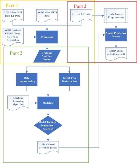
2.1. Methods

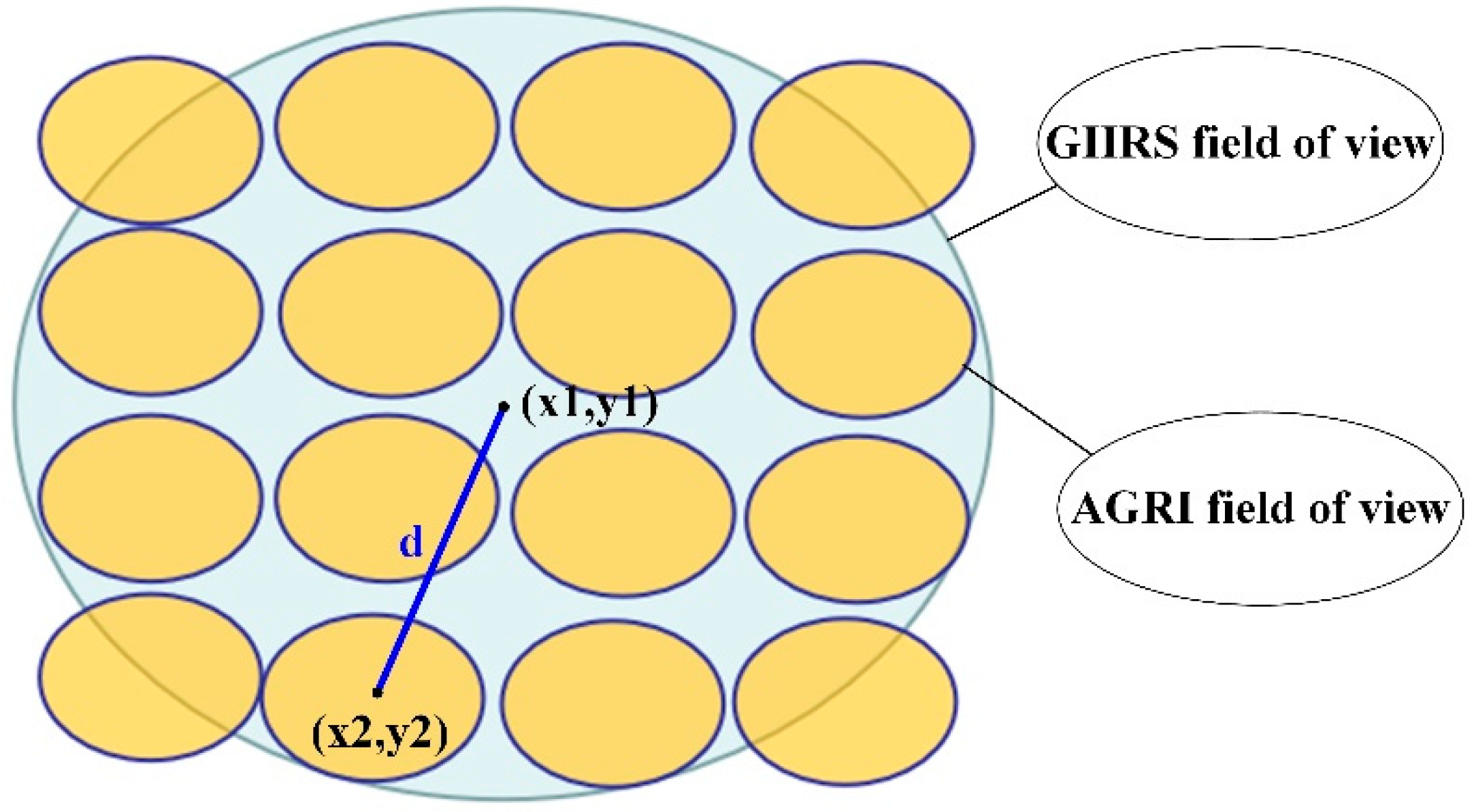
2.1.1. AGRI-GIIRS Cloud Detection Method

AGRI-GIIRS cloud detection was objectively determined using 4 km AGRI cloud detection products that fell in each GIIRS FOV. The AGRI FOV and the GIIRS FOV were regarded as two points on the earth sphere. It was considered that the AGRI FOV occurred in the GIIRS FOV when the distance between the two points was less than the radius of the GIIRS FOV. However, as the FOV of a detector is not always circular, the shape of FOV gradually becomes an egg shape which is difficult to describe mathematically, especially as the scanning angle increases. Considering deformation of the FOV, we set the distance threshold to 9 km, that is, the AGRI FOV fell in the GIIRS FOV when the distance between the two points was less 9 km. Finally, the cloud label of the GIIRS pixel was determined by the proportion of the clear AGRI FOVs and the cloud AGRI FOVs fell in the GIIRS FOV.

The specific steps used in the AGRI-GIIRS cloud detection method were:

1. Time matching

$$\left|t_{GIIRS}-t_{AGRI}\right|<{\delta }_{\max \_sec}$$

(1)

where, $t_{GIIRS}$ is the observation time of the GIIRS pixel; $t_{AGRI}$ is the observation time of the AGRI pixel; and ${\delta }_{\max \_sec}$ is 600 s.

2. Spatial matching

As shown in Figure 2, AGRI-GIIRS FOV pairs (x1, y2) and (x2, y2) were considered spatially matched when their distances satisfied Equations (2) and (3). Equation (2) calculates the distance between two points on a sphere, as:

$$\mathrm{d}=2R{\sin }^{-1}\sqrt{{(\sin \frac{x2-x1}{2})}^2+\cos x1\ast \cos x2\ast {(\sin \frac{y2-y1}{2})}^2}$$

(2)

$$\mathrm{d}<d_{max}$$

(3)

where, x1 is the central latitude of the GIIRS FOV; x2 is the central latitude of the AGRI FOV; y1 is the central longitude of the GIIRS FOV; y2 is the central longitude of the AGRI FOV; R is the radius of the earth (6371 km); and d_max is the distance threshold which is set at 9 km.

3. Determining the GIIRS FOV cloud label

According to Equations (2) and (3), 13–17 AGRI FOVs fell in each GIIRS FOV. The GIIRS FOVs are divided into three class: (1) a GIIRS FOV was considered to have a cloud label (label = 0) if all of the AGRI labels were cloud; (2) a GIIRS FOV was considered to have a clear label (label = 1) if all of the AGRI labels were clear; (3) a GIIRS FOV was considered to have a partially cloudy label (label = 2) if any cloud FOV and clear FOV of AGRI fell into the GIIRS FOV at the same time.

The GIIRS FOV was eliminated when AGRI FOVs that fell in the GIIRS FOV satisfied the following conditions:

(1)

all AGRI FOVs were probably clear or probably cloud.

(2)

some AGRI FOVs were probably cloud or probably clear, while others were clear or cloud.

Cloud labels defined by GIIRS using the AGRI-GIIRS cloud detection method are shown in Figure 3c, and the missing points are GIIRS FOVs that satisfy the above two conditions. Here, red dots represent clear FOVs, the blue dots represent cloud FOVs and green dots represent partially cloudy FOVs. Results indicate that the cloud label obtained using the matching method was consistent with the visible cloud image (Figure 3a) and the cloud detection product of AGRI AGRI (Figure 3b).

2.1.2. Machine Learning Cloud Detection Method

First of all, it needs to be emphasized that we established three kinds of datasets, each of which was divided into training set and test set. The first data set contained only totally cloudy and totally clear GIIRS FOVs, called training set 1 and test set 1. The second kind of dataset regarded totally cloudy and partially cloudy GIIRS FOVs as cloud GIIRS FOVs (label = 0), called training set 2 and test set 2. The third data set divided GIIRS pixels into three categories (totally clear, partially cloudy, and totally cloudy), which was called training set 3 and test set 3.

In this paper, the machine learning cloud detection method regards GIIRS pixel cloud detection as a binary classification problem, with a 0 value indicating a cloud FOV and a 1 value of indicating a clear FOV. The cloud detection model and results shown in the experiments and results (Section 3, Section 4) only used the data from training set 1 and test set 1. However, the effect of the model proposed in this paper on test set 2 was evaluated in Section 5.5. Section 5.5 also discussed the binary classification cloud detection model using training set 2 and the multi-classification cloud detection model using training set 3.

Currently there are many effective supervised machine learning algorithms for binary classification problems, such as random forest, Super Vector Machine (SVM), and logistic regression. For supervised algorithms, training datasets and test datasets are key processes in these methods. It is important that both datasets must include the FOV cloud label and the corresponding model input features. In our investigation, the cloud label derived from the AGRI-GIIRS cloud detection method, however we only retained GIIRS FOVs labeled 0 and 1. The radiation observations of GIIRS long wave infrared channels were taken as the features. The purpose of this method was to train the machine learning cloud detection model. Here, the cloud label of any GIIRS FOV can be obtained by inputting the channel radiation observations into the established model.

The specific steps of the machine learning cloud detection algorithm were:

1. Selection of machine learning algorithm for cloud detection

Logistic regression is suitable for fast binary classification [40,41]. which has been widely used in data mining and classification [42]. In the field of cloud detection, Luo [26] used the logistic regression method for IASI cloud detection, obtaining robust results for sea areas with a test accuracy of 97%. Equation (4) is the cost function of the logistic regression, which consists of two terms, the first term is the loss function, and the second term is the regular term:

$$\mathrm{J}\left(\mathsf{\theta }\right)=-\frac{1}{N}{{\displaystyle \sum }}^{\text{}}\log \left(1/\left(1+e^{-\left({\theta }^{T}x\right)}\right)\right)+\left(1-y\right)\log \left(1-1/\left(1+e^{-\left({\theta }^{T}x\right)}\right)\right)+C{\left|\right|\theta \left|\right|}_p$$

(4)

where, ${\theta }^T$ is the coefficient of logical regression discriminant function; and C is the penalty coefficient, which is the inversion of regularization strength, smaller values specifying stronger regularization and indicating a more simple model.

When p = 1, L1 regularization [43,44] occurs, and when p = 2, L2 regularization [44] occurs. L1 regularization can achieve the purpose of feature selection through sparse features; both regularization methods can avoid overfitting. For small sample data sets, L1 regularization can be iterated using the “liblinear” [45] method to optimize the loss function, and L2 regularization can be optimized using the “newton-cg” [46], “lbfgs” [47], and “liblinear” methods.

The underlying surface on land is more complex, therefore the accuracy of logical regression on the land test set declined to 88%, thus other algorithms were considered. Commonly used ensemble learning methods, such as random forest [48], adaboost [49,50], extremely randomized tree [51], and gradient boosting decision tree [52] are composed of multiple decision trees, which usually have better results than those using a single model. In addition, extremely randomized tree is more random in selecting and dividing nodes, resulting in a better generalization effect [53].

Finally, we selected the logistic regression (lr) model for cloud detection over sea and the extremely randomized tree (et) model for areas over land.

2. Model feature selection

GIIRS long-wave infrared radiation observations of different channels were selected in this study as the feature input of the cloud detection model. This selection was made as absorption and scattering spectra of clouds have relatively limited local spectral variation at 10–15 microns, and cloud-sensitive long-wave infrared radiation observations can be used to retrieve the cloud top height and effective cloud emissivity of monolayer clouds [54].

Two kinds of training sets were constructed in this study, differing only in channel selection. The first set used all 689 channels of GIIRS long wave infrared. The other set used 38 channels, including 35 long wave infrared channels, selected by Han [55], by analyzing GIIRS channel observation errors and channel noise and three other window channels. The number of training samples are shown in

Table 1. Hyperparameters of the two models.

Model	C	n_estimators	max_depth	max_features	min_samples_leaf	Min_samples_split
lr	✓	-	-	-	-	-
et	-	✓	✓	✓	✓	✓

.

3. Data preprocessing

In logistic regression, if regularization is used, the features must be standardized. The regularization term prevents overfitting by punishing large parameters. If the features are not standardized, those with larger values tend to get greater weights. The regularization term forces the norm of the large parameters to be as small as possible, however small parameters are ignored. Based on this experience, the normal distribution of eigenvalues was standardized in this study, as

$${\mathrm{X}}_{\mathrm{Standardization}}=\left(\mathrm{X}-\mathsf{\mu }\right)/\mathsf{\sigma }$$

(5)

4. Model performance assessment and hyperparameter tuning

Figure 4 is the confusion matrix of cloud detection classification [48]. Based on confusion matrix, five performance metrics were calculated: accuracy Equation (9), Probability Of Detection (POD; Equation (10)), False Alarm Rate (FAR; Equation (11)), Heidke Skill Score (HSS; Equation (12)) [56], and Area Under the ROC Curve (AUC; Equation (8)) [57,58].

AUC score was selected to measure models’ performance in the process of model tuning. When the number of positive and negative samples are not balanced, ROC has an advantage as it remains the same. In ROC, the x-axis is a False Positive Rate (FPR; Equation (6)) and the y-axis is a True Positive Rate (TPR; Equation (7)). Performance of the model is better when FPR is closer to 0 and TPR is closer to 1. AUC is defined as the area between the ROC curve and the x-axis, having a probability value between 0 and 1. The larger the AUC value is, the more likely the model is to put the positive sample in front of the negative sample when given a positive sample.

In the experimental results section, accuracy, POD, FAR, and HSS were used to evaluate the classification effect of the model. HSS eliminate forecasts which would be correct due to random chance (range from $-\infty$ to 1, with ‘0’ indicating no skill and ‘1’ indicating perfect score).

FPR = FP/(FP + TN)

(6)

TPR = TP/(TP + FN)

(7)

$$\mathrm{AUC}={{\displaystyle \int }}^{\text{}}ROC$$

(8)

Accuracy = TP + TN/(TP + TN + FP + FN)

(9)

POD = TP/(TP + FN)

(10)

FAR = FP/(FP + TP)

(11)

HSS = 2(TP*TN−FP*FN)/((TP + FN)*(TN + FP)+(TP + FP)*(TN + FN))

(12)

The trend of the effect of the model with the number of training sample numbers can indicate the state of the model (over-fitting/underfitting), and indicate what training sample size is needed for the corresponding classification problem. Only after understanding the state of the model is it possible to tune the hyperparameters of the model. In Section 3.3., the learning-curve [59] is selected to finish this part.

In machine learning, hyperparameters are critical as different hyperparameters often result in models having significantly different performances [60]. Parameters are usually selected by setting different values and training different models. As there were five parameters (Table 1) that needed to be tuned at the same time in the extremely randomized tree, the “grid search” [61] method was used to select a parameter combination with the best classification effect. Among all the candidate parameters, the “grid search” method identified the parameter combination with the greatest evaluation score by traversing each set of parameter combinations.

Based on the prediction probability (p) and the probability threshold θ, logistic regression and extremely randomized tree were used to classify each FOV. If $\mathrm{p}\ge \mathsf{\theta }$, the cloud label of the FOV was 1, representing a clear FOV; if $\mathrm{p}<\mathsf{\theta }$, the cloud label of the FOV was 0, representing a cloud FOV. Although the default value of $\mathsf{\theta }$ was 0.5, it was not always the best threshold for every classification problem. In this study, the confusion matrix [62] (Figure 4) was used as a guide to select the right probability threshold of cloud detection machine learning model. Composition of the confusion matrix indicates that changing the classification threshold will result in changes in TP, FN, FP, and TN. When the ratio of TP to TN was closer to 1, and the ratio of FN to FP was closer to 0, the classification threshold was considered to be more appropriate.

2.2. Data and Materials

2.2.1. Input Data of the AGRI-GIIRS Cloud Detection Method

GIIRS is one of the key payloads on FY-4A, and Michelson interference spectroscopy was used to observe three spectral bands: medium wave infrared (MW) band, long wave infrared (LW) band and visible (VIS) band. GIIRS has 689 LW channels measuring from 700 to 1130 cm⁻¹, 981 MW channels measuring from 1650 to 2250 cm⁻¹ and one visible light channel measuring from 0.55 to 0.75 $\mathsf{\mu }\mathrm{m}$. For the infrared channels, GIIRS records 60 earth observation residence points per observation period, and each residence point contains 128 probe elements arranged in a 32*4 formation, providing infrared information at a 16 km horizontal resolution at nadir with a spectral resolution of 0.625 cm⁻¹. Cloud reflection and radiation emission is recorded by GIIRS using the LW band, containing a window band ranging from 8.84 to 12 $\mathsf{\mu }\mathrm{m}$. Channels in this band were therefore selected as the input features of the model.

AGRI, another main load of FY-4A, is equipped with 14 channels, including the visible light band, the near infrared band, the short wave infrared band, the medium wave infrared band, and the long wave infrared band. Using AGRI not only enables a panoramic view of large scale weather systems to be observed, it also enables observation of rapid evolution processes of medium and small scale weather systems. AGRI level 2 product CLoudMask (CLM) was generated by performing 13 spectral and spatial uniformity tests and 2 restore tests [63]. Cloud labels for AGRI FOV were divided into four categories in CLM: cloud (label = 0), probably cloud (label = 1), probably clear (label = 2), and clear (label = 3). The MODIS products have been well validated through comparison with activate remote sensing data and radiance simulations [64,65,66], its Collection 6 (C6) cloud mask product is commonly used as the benchmark or truth for evaluating the performance of new cloud mask algorithms [67,68]. Lai [69] compared AGRI CLM product with MODIS C6 cloud mask product, and the result showed that the AGRI fractions are quite similar to the MODIS results with differences of less than 2% in the four categories.

2.2.2. Input Data for the Machine Learning Cloud Detection Algorithm

• When training machine learning cloud used the detection model, the real cloud label of GIIRS FOV was obtained using the AGRI-GIIRS cloud detection algorithm (0 for cloud GIIRS FOVs and 1 for clear GIIRS FOVs) and the GIIRS channels observation data were used as input features.
• When using the established machine learning cloud detection model, GIIRS data were processed into the file which conformed to the model input format through the preprocessing program as the input.

2.2.3. Auxiliary Validation Data

In the result verification phase, the cloud detection results of the machine learning cloud detection model was verified by comparing the visualized cloud detection results with the cloud images of AHI [70].

Three visible light and three near infrared bands were used in the visible light cloud image: red light (0.47 μm), green light (0.51 μm), and blue light (0.64 μm) in the visible light band and channel 4 (0.86 μm), channel 5 (1.6 μm), and channel 6 (2.3 μm) in the near infrared band. Infrared cloud images use channel 11 (8.6 μm), channel 12 (9.6 μm), channel 13 (10.4 μm), channel 14 (11.2 μm), channel 15 (12.4 μm), and channel 16 (13.3 μm).

3. Machine Learning Cloud Detection Experiment

3.1. Training Data and Test Data

We studied the scan range of the GIIRS (Figure 5). A scanning period consisted of seven time periods corresponding to different scanning regions.

The land training set and test set selected in our study were distributed in area A, corresponding to time period T2. The ocean training set and test set are distributed in area B, corresponding to the time periods T4 and T5. Spatial applicability of the model was verified using areas C and D (see Section 5.2.2).

The number of training samples and test samples for land and sea (with and without cloud cover) are listed in

Table 2. The number of training and test samples.

Type	Training Data	Test Data
sea_cloud	4254	1986
sea_clear	4855	1885
land_cloud	4301	2068
land_clear	4486	2081

. Test data are sampled from different seasons and different time of the day (

Table 3. Sampling time of the test samples.

Date(YYYY-MM-DD-HH:MM)	Land/Sea Flag	Day/Night Flag
2019-01-24-00:15	Land	Day
2019-05-14-12:15	Land	Night
2019-05-15-03:00	Land	Day
2019-06-15-12:15	Land	Night
2019-02-11-19:00	Sea	Night
2019-05-15-03:00	Sea	Day
2019-05-15-20:45	Sea	Night
2019-08-15-15:00	Sea	Night

).

3.2. Machine Learning Cloud Detection Model

Four models’ information are summarized in

Table 4. Information relating to the two machine learning models.

Model	Area	Input Features	Abbreviation	Data Solution
et	Land	689 channels	et(689 channels)	-
et	Land	38 channels	et(38 channels)	-
lr	Sea	689 channels	lr(689 channels)	Standardization
lr	Sea	38 channels	lr(38 channels)	Standardization

.

3.3. Model Parameter Tuning and Performance Evaluation

3.3.1. Sample Size

It is important to highlight that:

• The AUC score for the test data in this section was derived using a 5-fold cross-validation method;
• The shaded parts of Figure 6, Figure 7 and Figure 8 represent the dispersion of the score, having the following equation:

  $$\mathrm{Dispersion}=x_{mean}\pm \mu$$

  (13)

  where, $x_{mean}$ is the average score; and $\mathsf{\mu }$ is the standard deviation of the score.
• The default value was used for hyperparameters (e.g., C = 1).

1. Logistic regression.

Changes in AUC with different training sample numbers are shown in Figure 6. The first column used 689 channels as input features and the second column used 38 channels; the first row used L2 regularization and the second row used L1 regularization.

From Figure 6, we can infer that:

• All AUC scores in the four models (training and test data) tended to be stable when the sample number was greater than or equal to 4000, indicting that at least 4000 samples are required for 4 cloud detection models.
• The AUC score of lr (689 channels) (Figure 6b,d) on the training set was always higher than that of on the test set, indicating that the model was over-fitted. Generally speaking, over-fitting can be improved by increasing the amount of data, reducing the complexity of the model (stronger regularization) or reducing the number of model features. Compared with lr (689 channels) models, the score of lr (38 channels) models (Figure 6a,c) on the training set was the same as that on the test set when the number of training samples is more than 4000, which indicated that over-fitting phenomenon did disappear after reducing some features. Additionally, when the number of training samples increased from 4000 to 7000, the over-fitting phenomenon of the lr (689 channels) models still existed. Thus, increasing the number of training samples could not improve the over-fitting in this problem. In Section 3.3.2, hyperparameter ‘C’ was tuned to improve the over-fitting issue.
• For models with the same input features, L1 and L2 regularization almost scored the same when the AUC of the training set and test set were not changed with sample size.

2. Extremely Randomized Tree

Results for the extremely randomized tree AUC change trends (Figure 7) indicated stable trends when the sample size was greater than 6000. The AUC score of both models on the training set were always higher than those of on the test set, indicating that both models were over-fitted. Hyperparameters listed in Table 1 determined an extremely randomized tree’s architecture. Those hyperparameters needed to be tuned to improve over-fitting and models’ performance by changing the shape of the trees’ architecture.

3.3.2. Hyperparameters Tuning

1. Logistic regression

In the previous section, models with 689 channels recorded over-fitting. In addition, we were not aware whether models with 38 channels were underfitting. In order to solve these two problems and find the optimal hyperparameters for logistic regression models, we observed how the performance of the models changed when hyperparameter “C” ranged from 0.0001 to 1000 at intervals of 10 (Figure 8).

In Figure 7, parameter ‘C’ was set to default value ‘1’. In Figure 8a,c, it is clear that AUC score improved when C was greater than 1. The increase of C indicated that the intensity of regularization decreased and the complexity of the model increased. Thus, it can be inferred that there was a bit of underfitting of lr (38 channels) in Figure 7, and a bigger value for C (>1) could improve underfitting. Although the AUC score on the two data sets remained unchanged when C was greater than or equal to 10, the best value for ‘C’ was 10. The reason is that the larger the C is, the weaker the regularization is, so the higher the complexity of the model is, the worse the generalization ability of the model is. Considering that scores of the two regularization methods on the two training sets and test sets were similar, and L1 regularization can be used for feature selection, L1 regularization (C = 10) was selected for the logistic regression model in the following experiments.

2. Extremely randomized tree

Table 5. hyperparameters of the two extremely randomized tree models.

Model	n estimators	max features	max depth	n samples split	min samples leaf	AUC (origin)	AUC (tuned)
et (38channels)	100	20	5	2	1	0.975	0.980
et (689channels)	130	30	10	2	1	0.980	0.984

listed the optimal hyperparameters selected for two extremely randomized tree models. AUC score in the test set increased for both models after the parameters had been tuned by using “grid search” method.

3.3.3. Probability Threshold Tuning

By using the et (689 channels) model as an example, Figure 9 shows how the confusion matrix changed when the probability threshold (θ) ranged from 0.1 to 0.9. This result indicates that the best threshold was between 0.4 and 0.6, then we can get a better classification threshold by narrowing the interval between 0.4 and 0.6. The process of threshold selection for each model is not listed here, and

Table 6. Optimal classification thresholds for the four models.

et (38 channels)	et (689 channels)	lr (38 channels)	lr (689 channels)
0.55	0.6	0.98	0.98

lists the optimal probability thresholds of the four models.

4. Results

4.1. Statistics of Four Cloud Detection Models on Test Data

According to the statistical results listed in

Table 7. Test data statistics of the four models on the corresponding test set.

Model	POD	FAR	ACC	HSS
et(38 channels)	0.914	0.177	0.872	0.741
et(689 channels)	0.916	0.166	0.891	0.780
lr(38 channels)	0.986	0.071	0.956	0.912
lr(689 channels)	0.993	0.047	0.973	0.945

, four cloud detection models produced high accuracy, high POD, and low FAR from the test data statistics (Table 7), indicating their good performance for detecting clouds in the case of totally cloudy totally clear. In addition, the classification results of the 689 channels models were slightly better than those of the 38 channels models. Results for the logistic regression model showed a robust result for sea areas, with accuracy exceeding 95% and HSS exceeding 90% for both models. The Extremely randomized tree model also performed well on areas of land. Due to the complexity of the situation over the land, the effect of land cloud detection is lower than that of the sea surface.

4.2. Visualization Verification of The Model Classification Effect

In order to test the classification effect of the machine learning model in the complete sky scene, we selected six scenes (

Table 8. Site information for the six scenes.

Scene Number	Date (YYYY-MM-DD-HH:MM)	Day/Night Flag	Region	Land/Sea Flag	Characteristics
1	2019-08-16-08:15	Day	$80°\mathrm{E}–120°\mathrm{E},$ $36°\mathrm{N}–42.5°\mathrm{N}$	Land	Snow, Cloud Shadow
2	2019-08-20-04:15	Day	$80°\mathrm{E}–120°\mathrm{E},$ $36°\mathrm{N}–42.5°\mathrm{N}$	Land	Multi-layer Cloud
3	2019-08-18-12:15	Night	$80°\mathrm{E}–120°\mathrm{E},$ $36°\mathrm{N}–42.5°\mathrm{N}$	Land	-
4	2019-08-14-02:30	Day	$122°\mathrm{E}–142°\mathrm{E},$ $27.9°\mathrm{N}–34.4°\mathrm{N}$	Sea	Typhoon KROSA
5	2019-08-21-04:30	Day	$122°\mathrm{E}–142°\mathrm{E},$ $27.9°\mathrm{N}–34.4°\mathrm{N}$	Sea	Thin Cirrus, Broken Cloud
6	2019-08-08-12:45	Night	$120°\mathrm{E}–140°\mathrm{E},$ $21.5°\mathrm{N}–28°\mathrm{N}$	Sea	Typhoon LEKIMA

) to further verify the classification results of the model through visualization results.

In Figure 10, the six cloud images in the left column contain different types of clouds under different conditions. The middle column lists the classification results of the model using 38 channels, and the right column lists classification results of the model using 689 channels. With six cloud images as references, most of the cloud FOVs were correctly detected using the model incorporating two kinds of feature input. It is worth noting that both cloud detection models detected the majority of broken clouds floating on the snow surface (in the red circle) in Figure 10a1,a2. In addition, some of the mistakenly divided FOVs are circled in blue, and the correctly classified FOVs are circled in red. On the whole, the machine learning cloud detection model using the two feature input recorded good cloud detection capabilities.

5. Discussion

5.1. Time Complexity of AGRI-GIIRS Cloud Detection and Machine learning Cloud Detection

Time Complexity

Figure 11 shows the pseudocode of the AGRI-GIIRS cloud detection algorithm. Lines 1–14 retained only AGRI pixels covered in all GIIRS pixels area, and lines 19–30 calculated the distance between each GIIRS pixel and the reserved AGRI pixel, placing each AGRI pixel that fell within the GIIRS field of view into the list. The time complexity of the algorithm was $\mathrm{O}\left(M\ast N\left(1+10\ast N\right)\right)$, N is the number of GIIRS pixels $\left(la{t}_g,lo{n}_g\right)$; and M is the number of reserved AGRI pixels $\left(la{t}_{save},lo{n}_{save}\right)$. A GIIRS FOV can match 13–17 GIIRS pixels, therefore M is about 10 times that of N, so the algorithm complexity is $\mathrm{O}\left(N^3\right)$.

The essence of the training logistic regression model is to generate a set of characteristic coefficients and establish a good discriminant function. Therefore, when the logistic regression model is used, the channel observation value of each GIIRS pixel can be substituted into the established discriminant function, resulting in the complexity of the model to be O(P), P is the number of input feature channels. As the extremely randomized tree is composed of many decision trees, its prediction time complexity is O($N\ast p\ast n_{trees}$), where N is the input number of GIIRS pixels and $n_{trees}$ is the number of trees. The time complexity of the model is related to the structure of the tree (i.e., $n_{trees}$) which is a constant number.

The time complexity of the AGRI-GIIRS cloud detection method, logistic regression and extremely randomized tree are the input number of GIIRS pixels (N) to the power of three, N to the power of one and N to the power of 0, respectively. So it is clear that the cost of time of the AGRI-GIIRS cloud detection method increased faster than machine learning methods with the input number of GIIRS pixels (N).

We ran the AGRI-GIIRS cloud detection code and four machine learning cloud detection methods’ code on an 8G i5 computer (

Table 9. The average running time (ten times) of AGRI-GIIR cloud detection method.

Model	GIIRS FOV Number	Runtime
AGRI-GIIRS Cloud Detection	1280	265
	1920	600
	2560	885
et (38 channels)	1280	within 1.5 s
	1920
	2560
et (689 channels)	1280	within 1.5 s
	1920
	2560
lr (38 channels)	1280	within 0.15 s
	1920
	2560
lr (689 channels)	1280	within 0.2 s
	1920
	2560

). The average time cost of running the AGRI-GIIRS cloud detection method was significantly greater than time taken to run the machine learning cloud detection methods.

5.2. Applicability of The Machine Learning Cloud Detection Algorithm

5.2.1. Applicability of Time

Experimental results in Section 4 highlighted that the classification accuracy of the four machine learning cloud detection models was more than 90% in the test data covering winter, spring, and summer. In addition, visualization results showed that the cloud detection results for day and night were basically the same as the cloud images. This finding highlights that the machine learning cloud detection algorithm can detect clouds using GIIRS data in different seasons and different times of the day.

5.2.2. Spatial Applicability

The area selected for land training and the test set in this study was located between 35 °N and 45 °N. Compared with areas further south, surface vegetation coverage is lower, air humidity is smaller, and climate and topography are different. In order to investigate whether the model can achieve good cloud detection results in different regions, we tested the land model on 2179 test samples in areas further south (Area C in Figure 5) and the sea model on 1200 middle-high latitude sea areas (Area D in Figure 5). The accuracy of et (689 channels) and et (38 channels) on land test samples was 77.1% and 78.6%, respectively. The accuracy of lr (689 channels) and lr (38 channels) on sea test samples was 66.4% and 64.67%, respectively.

By adding the training samples to the training data within Areas C and D, the overall accuracy of the new model on the test data set was reduced by about 7%. Therefore, the machine learning cloud detection method, which only depends on GIIRS observation data, can achieve better cloud detection results if a separate model for the region of interest is established, however this is not a spatially universal method.

5.3. Comparison of Cloud Detection Methods Between Machine Learning Cloud Detection and Weather Research and Forecasting Model Data Assimilation System(WRFDA)

Currently, WRFDA is one of the most widely used assimilation systems. This system uses the following four criteria to determine whether Atmospheric Infrared Sounder (AIRS) pixels are contaminated by the cloud [71]:

• model cloud water path detection;
• 956 cm⁻¹ long wave window channel brightness temperature detection;
• sea surface temperature deviation detection;
• cloud cover area detection.

Except for observations, the first bullet point and the third bullet point also depend on the background field. When a large deviation in the background field occurs, criteria for cloud detection becomes unreliable. However, the machine learning cloud detection method, which uses GIIRS channel observations as features, only depends on the GIIRS observation data itself.

5.4. Channel Contribution

Figure 12 shows channels’ contribution in four cloud detection models. For lr (689 channels), most of the channels do not contribute to the cloud detection process with coefficient equal to 0. For et (689 channels), most of the channels’ importances were close to 0. However, almost all 38 channels made contributions to cloud detection in lr (38 channels) and et (38 channels). In addition, the average difference between model accuracy for 38 channels and 689 channels was about 0.02 (Table 7), indicating that even a small number of accurate channel observations can achieve cloud detection results similar to those using all 689 channels.

5.5. Limitations and some Exploration of Machine Learning Cloud Detection Method

5.5.1. Model Applicable Scenario

The method proposed in this paper performed well when the GIIRS pixel was totally cloudy or totally clear. Due to the technical limitation, the HIR data characterized with high spectral resolution and low spatial resolution, so it is inevitable that many pixels are partially cloudy.

Therefore, in this section, the following two parts are discussed:

• Can the model established above separate partially cloudy GIIRS FOVs from the totally clear GIIRS FOVs?

We added 1214 partial cloud test samples to the original sea test set (Table 2), 1109 partially cloudy test samples to the original land test set (Table 2), then we set the label of partially cloudy test samples to ‘0’. Therefore, there were still two types of FOVs (cloudy FOVS and totally clear FOVs) in the test set, and the statistical results are listed in the

Table 10. Statistical results of 4 established models on new test set.

Model	POD	FAR	ACC	HSS
et (38 channels)	0.902	0.460	0.749	0.432
et (689 channels)	0.912	0.431	0.775	0.501
lr (38 channels)	0.873	0.376	0.766	0.527
lr (689 channels)	0.929	0.36	0.787	0.504

. The FAR of the four models increased significantly compared to statistical results in Table 7, indicating that many partially cloudy FOVs were misjudged as totally clear FOVs. Accuracy and HSS also decreased significantly. It showed that the model established in this paper was still difficult to distinguish between partially cloudy FOVs and totally clear FOVs.

• Can adding some cloud pixels to the training set improve the effect of the model recognition part with cloud pixels?

GIIRS’s cloud labels were classified into three categories (these three types of cloud labels are defined in Section 2.1.1, point 3.). Two kinds of models (

Table 11. Training sets’ cloud labels and sample size of two kinds of models.

	Cloud			Clear			Partial Cloud
	Label	Training Samples		Label	Training Samples		Label	Training Samples
		Sea	Land		Sea	Land		Sea	Land
Model_1	0	7000	9300	1	7000	9300	2	6830	9202
Model_2	0	7000	9300	1	14,500	16,595	0	6830	9202

) were constructed using the training sets of different label combinations: the first model was a three-class classification model (totally clear, partially cloudy, totally cloudy); the second model was a binary-classification model, which regarded the totally clear sky FOVs as one class, and the totally cloudy and partially cloudy FOVs together as the second class. After selecting the appropriate number of training samples and adjusting the parameters as described in Section 3.3, the two kinds of models’ classification results were listed in

Table 12. Two kinds of models’ statistical results.

Type	model	region	input features	ACC	HSS
Three-Class Classification	Model_1	Land	38 channels	0.562	0.334
	Model_1	Land	689 channels	0.571	0.351
	Model_1	Sea	38 channels	0.644	0.438
	Model_1	sea	689 channels	0.736	0.604
Binary Classification	Mdoel_2	Land	38 channels	0.783	0.401
	Model_2	Land	689 channels	0.797	0.511
	Model_2	Sea	38 channels	0.762	0.467
	Model_2	sea	689 channels	0.769	0.545

. Both of the models were based on extremely randomized tree. From the scores of ACC and HSS (see [56] for multi-classification HSS calculation), the classification effects of the two models were no better than those of the original model. The two models were also trained based on the logistic regression algorithm, while the statistical results were no better than Table 12 and were not listed here. Whether the recognition effect of partially cloud FOVs can be enhanced by using other machine learning algorithms or adding other feature input needs to be further studied.

Based on the discussion above, the method proposed in this paper is not effective in distinguishing partially cloudy FOVs. It is suitable for situations where the distribution of clouds in the sky is relatively concentrated (such as scene 1, scene 2, scene 3, scene 4, scene 5, scene 7 in Figure 10). Under such situation, there are more FOVs of totally cloudy and totally clear skies, while partially cloudy FOVs are relatively few.

5.1.2. The Reliability of Training Set and Test Set

Supervised machine learning depends heavily on the correctness of the label. This article treats AGRI’s CLM product as reference data. Although this product had validated with MODIS cloud product, there was no guarantee that the training data label retrieved from AGRI in the selected time period was correct. In the training set, the wrong GIIRS FOVs added noise in the process of building the model. In the test set, the GIIRS FOVs with the wrong labels might affect the selection of the classification threshold, which would directly lead to misclassification. In addition, when the GIIRS FOV was not located at the nadir point, the deformation of FOV occurred, and the situation of GIIRS matching AGRI became more complex, so the method of matching two FOVs according to distance also had uncertainty.

6. Conclusions

It has been noted that weather forecasting can only be significantly improved when the detection accuracy of global atmospheric vertical temperature and humidity profiles attain the level of radio sounding. Infrared hyperspectral data play an important role in the retrieval of temperature and humidity profiles by virtue of its hyperspectral resolution. GIIRS, the first infrared hyperspectral sounders attached to a geostationary satellite, can provide high frequency observation information and track major weather processes. The use of GIIRS data will inevitably improve forecasting ability.

However, current methods using cloudy hyperspectral data is still an important issue. Commonly used methods used to identify cloud FOVs include the clear sky channel cloud detection algorithm and the optimal cloud clearing algorithm. However, before these methods are used for cloud FOVs, it is necessary to correctly distinguish between cloud FOVs and clear FOVs.

In this study, a machine learning cloud detection method for infrared hyperspectral data was proposed. Due to noticeable differences between sea and land, cloud detection models have been established for each area separately. Four machine learning models were trained with 689 channel observations and 38 channel observations as features, and cloud labels were obtained by AGRI-GIIRS matching algorithm as truth values. After selecting the appropriate classification threshold, sea test data using the lr (689 channels) model and the lr (38 channels) model attained accuracy levels of 97.3 and 95.6%, respectively. The land test data set using the et (689 channels) model and the et (38 channels) model attained an accuracy level of 89.1 and 87.2%, respectively.

In addition, six real cloud scenes were randomly selected over areas of land and sea to verify results gained using the machine learning cloud detection method. The machine learning method showed good performance in distinguishing clouds and the underlying surface covered by snow, distinguish the boundary between clouds and clear skies, depict the two-dimensional shape of typhoon, and correctly identify some broken clouds.

Compared with the AGRI-GIIRS cloud detection algorithm, the machine learning cloud detection method significantly reduces time costs. Compared with the cloud detection settings in WRFDA, the machine learning cloud detection method only depends on real observations of GIIRS, thereby avoiding uncertainty caused by background fields. Our experimental results have also shown that cloud detection accuracy can be achieved by using only a small number of effective channels. Although this method has a good classification result for different periods of the day and different seasons of the year, there are some limitations to this study. First of all, this method is effective for the detection of totally cloudy and totally clear GIIRS FOVs, but not for partially cloudy FOVs, so it is suitable for cases where the distribution of clouds in the sky is relatively concentrated, where the portion of partially cloudy FOVs is small. Secondly, the spatial universality of the non-training area is poor. In particular, a partly cloudy FOV is required in some algorithms (e.g., optimal cloud clearing algorithm), so it is not enough to regard the cloud detection as a binary classification problem. Future research includes: (1) developing cloud detection method with spatio-temporal information to improve spatial limitation; (2) dividing cloud FOVs into two categories: fully cloud and partly cloudy; (3) developing cloud phase detection model using machine learning algorithms with the help of other observation data.

References

1. Aumann, H.H.; Miller, C.R. Atmospheric infrared sounder (AIRS) on the earth observing system. Proc. SPIE, Int. Soc. Opt. Eng. 1995, 2583, 332–343. [Google Scholar]
2. Smith, N.; Smith, W.L.; Weisz, E.; Revercomb, H.E. AIRS, IASI and CrIS retrieval records at climate scales: An investigation into the propagation systematic uncertainty. J. Appl. Meteorol. Climatol. 2015, 54, 1465–1481. [Google Scholar] [CrossRef]
3. Clerbaux, C.; Hadji-Lazaro, J.; Turquety, S.; George, M.; Coheur, P.F.; Hurtmans, D.; Wespes, C.; Herbin, H.; Blumstein, D.; Tourniers, B.; et al. The IASI/MetOp 1 mission: First observations and highlights of its potential contribution to GMES 2. Space Res. Today 2007, 168, 19–24. [Google Scholar] [CrossRef]
4. Smith, A.; Atkinson, N.; Bell, W.; Doherty, A. An initial assessment of observations from the Suomi-NPP satellite: Data from the Cross-track Infrared Sounder (CrIS). Atmos. Sci. Lett. 2015, 16, 260–266. [Google Scholar] [CrossRef]
5. Li, Z.; Li, J.; Wang, P.; Lim, A.; Li, J.; Schmit, T.J.; Atlas, R.; Boukabara, S.A.; Hoffman, R. Value-added impact of geostationary hyperspectral infrared sounders on local severe storm forecasts—Via a quick regional OSSE. Adv. Atmos. Sci. 2018, 35, 1217–1230. [Google Scholar] [CrossRef]
6. Lu, F.; Zhang, X.; Chen, B.; Liu, H.; Wu, R.; Han, Q.; Feng, X.; Li, J.; Zhan, Z. FY-4 geostationary meteorological satellite imaging characteristic and its application prospects. J. Mar. Meteorol. 2017, 37, 1–12. [Google Scholar]
7. Yang, J.; Zhang, Z.; Wei, C.; Lu, F.; Guo, Q. Introducing the new generation of Chinese geostationary weather satellites, Fengyun-4(FY-4). Bull. Am. Meteorol. Soc. 2016, 98, 1637–1658. [Google Scholar] [CrossRef]
8. Chen, W. Satellite Meteorology; China Meteorological Press: Beijing, China, 2003. [Google Scholar]
9. Dong, C.; Li, J.; Zhang, P. The Principle and Application of Satellite Hyperspectral Infrared Atmospheric Remote Sensing; Science Press: Beijing, China, 2013. [Google Scholar]
10. Wylie, D.P.; Menzel, W.P.; Woolf, H.M.; Strabala, K.I. Four years of global cirrus cloud statistics using HIRS. J. Clim. 1994, 7, 1972–1986. [Google Scholar] [CrossRef] [Green Version]
11. Li, J.; Liu, C.; Huang, H.; Schmit, T.J.; Wu, X.; Menzel, W.P.; Gurka, J.J. Optimal cloud-clearing for AIRS radiances using MODIS. IEEE Trans. Geosci. Electron. 2005, 43, 1266–1278. [Google Scholar]
12. McNally, A.P.; Watts, P.D. A cloud detection algorithm for high-spectral-resolution infrared sounders. Q. J. R. Meteorol. Soc. 2003, 129, 3411–3423. [Google Scholar] [CrossRef]
13. Rossow, W.B.; Garder, L.C. Cloud detection using satellite measurements of infrared and visible radiances for ISCCP. J. Clim. 1993, 12, 2341–2369. [Google Scholar] [CrossRef]
14. Rossow, W.; Mosher, F.; Kinsella, E.; Arking, A.; Desbois, M.; Harrison, E.; Minnis, P.; Ruprecht, E.; Seze, G.; Simmer, C.; et al. ISCCP cloud algorithm intercomparison. J. Appl. Meteorol. 1985, 24, 184–192. [Google Scholar] [CrossRef] [Green Version]
15. Kriebel, K.T.; Gesell, G.; Kastner, M.; Mannstein, H. The cloud analysis tool APOLLO: Improvements and validations. Int. J. Remote Sens. 2003, 24, 2389–2408. [Google Scholar] [CrossRef]
16. Stowe, L.L.; Davis, P.A.; Mcclain, E.P. Scientific basis and initial evaluation of the CLAVR-1 global clear/cloud classification algorithm for the advanced very high resolution radiometer. J. Atmos. Ocean. Technol. 1999, 16, 656–681. [Google Scholar] [CrossRef]
17. Baum, B.A.; Arduini, R.F.; Wielicki, B.A.; Minns, P.; Tsay, S.C. Multilevel cloud retrieval using multispectral HIRS and AVHRR data: Nighttime oceanic analysis. J. Geophys. Res. Atmos. 1994, 99, 5499–5514. [Google Scholar] [CrossRef]
18. Ackerman, S.A.; Strabala, K.I.; Menzel, W.P.; Frey, R.A.; Moeller, C.C. Discriminating clear sky from clouds with MODIS. J. Geophys. Res. 1998, 103, 32141. [Google Scholar] [CrossRef]
19. Ackerman, S.A.; Holz, R.E.; Frey, R.; Eloranta, E.W.; Maddux, B.C.; McGill, M.R. Cloud detection with MODIS. Part II: Validation. J. Atmos. Ocean. Technol. 2010, 25, 1073–1086. [Google Scholar] [CrossRef] [Green Version]
20. Li, J.; Menzel, P.W.; Sun, F.; Schmit, T.J.; Gurka, J.J. AIRS subpixel cloud characterization using MODIS cloud products. J. Appl. Meteorol. 2004, 43, 1083–1094. [Google Scholar] [CrossRef]
21. Eresmaa, R. Imager-assisted cloud detection for assimilation of infrared atmospheric sounding interferometer radiances. Q. J. R. Meteorol. Soc. 2014, 140, 2342–2352. [Google Scholar] [CrossRef]
22. Ma, Y.; Wu, H.; Wang, L.; Huang, B.; Ranjan, R.; Zomaya, A.; Jie, W. Remote sensing big data computing: Challenges and opportunities. Future Gener. Comput. Syst. 2014, 51, 47–60. [Google Scholar] [CrossRef]
23. Qiu, J.; Wu, Q.; Ding, G.; Xu, Y.; Feng, S. A survey of machine learning for big data processing. EURASIP J. Adv. Signal Process. 2016, 2016, 67. [Google Scholar] [CrossRef] [Green Version]
24. Li, P.; Dong, L.; Xiao, H.; Xu, M. A cloud image detection method based on SVM vector machine. Neurocomputing 2015, 169, 34–42. [Google Scholar] [CrossRef]
25. Bai, T.; Li, D.; Sun, K.; Chen, Y.; Li, W. Cloud detection for high-resolution satellite imagery using machine learning and multi-feature fusion. Remote Sens. 2016, 8, 715. [Google Scholar] [CrossRef] [Green Version]
26. Luo, T.; Zhang, W.; Yu, Y.; Feng, M.; Duan, B.; Xing, D. Cloud detection using infrared atmospheric sounding interferometer observations by logistic regression. Int. J. Remote Sens. 2019, 40, 1–12. [Google Scholar] [CrossRef]
27. Han, B.; Kang, L.; Song, H. A fast cloud detection approach by integration of image segmentation and support vector machine. In Proceedings of the International Symposium on Neural Networks, Chengdu, China, 28 May–1 June 2006. [Google Scholar]
28. Latry, C.; Panem, C.; Dejean, P. Cloud detection with SVM technique. In Proceedings of the IEEE Geoscience and Remote Sensing Symposium, Barcelona, Spain, 23–28 July 2007. [Google Scholar]
29. Xu, L.; Wong, A.; Clausi, D.A. A novel Bayesian spatial-temporal random field model applied to cloud detection from remotely sensed imagery. IEEE Trans. Geosci. Remote Sens. 2017, 55, 4913–4924. [Google Scholar] [CrossRef]
30. Li, Q.; Lu, W.; Yang, J.; Wang, J.Z. Thin cloud detection of all-sky images using Markov random fields. IEEE Geosci. Remote Sens. Lett. 2012, 9, 417–421. [Google Scholar] [CrossRef]
31. Yang, J.; Guo, J.; Yue, H.; Liu, Z.; Hu, H.; Li, K. CDnet: CNN-based cloud detection for remote sensing imagery. IEEE Trans. Geosci. Remote Sens. 2019, 99, 1–17. [Google Scholar] [CrossRef]
32. Mohajerani, S.; Saeedi, P. Cloud-net: An end-to-end cloud detection algorithm for Landsat 8 imagery. arXiv 2019, arXiv:1901.10077. [Google Scholar]
33. Xie, F.; Shi, M.; Shi, Z.; Yin, J.; Zhao, D. Multilevel cloud detection in remote sensing images based on deep learning. IEEE J. Sel. Topics Appl. Earth Obs. Remote Sens. 2017, 10, 3631–3640. [Google Scholar] [CrossRef]
34. Mohajerani, S.; Krammer, T.A.; Saeedi, P. A cloud detection algorithm for remote sensing images using fully convolutional neural networks. In Proceedings of the 20th IEEE International Workshop on Multimedia Signal Processing, Cape Town, South Africa, 21–24 October 2018. [Google Scholar]
35. Zhang, Z.; Iwasaki, A.; Song, J. Small satellite cloud detection based on deep learning and image compression. Preprints 2018. [Google Scholar] [CrossRef]
36. Sim, S.; Im, J.; Park, S.; Park, H.; Ahn, M.W.; Chan, P. Icing detection over East Asia from geostationary satellite data using machine learning approaches. Remote Sens. 2018, 4, 631. [Google Scholar] [CrossRef] [Green Version]
37. Han, D.; Lee, J.; Im, J.; Sim, S.; Lee, S.; Han, H. A novel framework of detecting convective initiation combining automated sampling, machine learning, and repeated model tuning from geostationary satellite data. Remote Sens. 2019, 12, 1454. [Google Scholar] [CrossRef] [Green Version]
38. Han, H.; Lee, S.; Im, J.; Kim, M.; Lee, M.; Ahn, M.; Chung, S. Detection of convective initiation using meteorological imager onboard communication, ocean, and meteorological satellite based on machine learning approaches. Remote Sens. 2015, 7, 9184–9204. [Google Scholar] [CrossRef] [Green Version]
39. Kim, M.; Im, J.; Park, H.; Park, S.; Lee, M.; Ahn, M. Detection of tropical overshooting cloud tops using Himawari-8 imagery. Remote Sens. 2017, 7, 685. [Google Scholar] [CrossRef] [Green Version]
40. Kleinbaum, D.G.; Klein, M. Logistic Regression (A Self-Learning Text); Springer: Berlin/Heidelberg, German, 2002. [Google Scholar]
41. Liao, J.G.; Chin, K.V. Logistic Regression for Disease Classification Using Microarray Data; Oxford University Press: Oxford, UK, 2007. [Google Scholar]
42. Komarek, P. Logistic Regression for Data Mining and High Dimensional Classification. Ph.D. Thesis, Carnegie Mellon University, Pittsburgh, PA, USA, 2004. [Google Scholar]
43. Koh, K.; Kim, S.J.; Boyd, S.P. A method for large-scale L1-regularized logistic regression. In Proceedings of the Twenty-Second AAAI Conference on Artificial Intelligence, Vancouver, BC, Canada, 22–26 July 2007. [Google Scholar]
44. Andrew, Y.N. Feature selection, L1 vs. L2 regularization, and rotational invariance. In Proceedings of the International Conference on Machine learning, Louisville, KY, USA, 16–18 December 2004. [Google Scholar]
45. Fan, R.E.; Chang, K.W.; Hsieh, C.J.; Wang, X.R.; Lin, C.J. Liblinear: A library for large linear classification. J. Mach. Learn. Res. 2008, 9, 1871–1874. [Google Scholar]
46. Gill, P.E.; Murray, W. Quasi-Newton methods for unconstrained optimization. IMA J. Appl. Math. 1972, 9, 91–108. [Google Scholar] [CrossRef]
47. Liu, D.C.; Nocedal, J. On the limited memory BFGS method for large scale optimization. Math. Program. 1989, 45, 503–528. [Google Scholar] [CrossRef] [Green Version]
48. Breiman, L. Random forests. Mach. Learn. 2001, 45, 5–32. [Google Scholar] [CrossRef] [Green Version]
49. Schapire, R.E. Explaining AdaBoost. In Empirical Inference; Springer: Berlin/Heidelberg, Germany, 2013. [Google Scholar]
50. Collins, M.; Schapire, R.E.; Singer, Y. Logistic regression, AdaBoost and Bregman distances. Mach. Learn. 2001, 48, 253–285. [Google Scholar] [CrossRef]
51. Geurts, P.; Ernst, D.; Wehenkel, L. Extremely randomized trees. Mach. Learn. 2006, 63, 3–42. [Google Scholar] [CrossRef] [Green Version]
52. Jerome, H.F. Greedy function approximation: A gradient boosting machine. Ann. Stat. 2001, 29, 1189–1232. [Google Scholar]
53. Goetz, M.; Weber, C.; Bloecher, J.; Stieltjes, B.; Meinzer, H.P.; Maier-Hein, K. Extremely randomized trees based brain tumor segmentation. In Proceedings of the MICCAI BraTS (Brain Tumor Segmentation Challenge), Boston, MA, USA, 14–18 September 2014. [Google Scholar]
54. Guan, L.; Xiao, W. Retrieval of cloud parameters using infrared hyperspectral observations. Chin. J. Atmos. Sci. 2007, 31, 1123–1128. (In Chinese) [Google Scholar]
55. Han, W. Assimilation of GIIRS radiances in GRAPES. In Proceedings of the 35th Chinese Meteorological Society Conference, Hefei, Anhui, China, 23–26 October 2019. [Google Scholar]
56. Bradley, P. The use of the area under the ROC curve in the evaluation of machine learning algorithms. Pattern Recogn. 1996, 30, 1145–1159. [Google Scholar] [CrossRef] [Green Version]
57. Nurmi, P. Recommendations on the Verification of Local Weather Forecasts; ECMWF Technical Memoranda 430 European Centre for Medium-Range Weather Forecasts (ECMWF): Reading, UK, 2003. [Google Scholar]
58. Alberto, J.V. Insights into the area under the receiver operating characteristic curve (AUC) as a discrimination measure in species distribution modelling. Glob. Ecol. Biogeogr. 2011, 21, 498–507. [Google Scholar]
59. Cortes, C.; Jackel, L.; Solla, S.A.; Vapnik, V.; Denker, J. Learning curves: Asymptotic values and rate of convergence. In Proceedings of the 7th Advances in Neural Information Processing Systems 6, Denver, CO, USA, 1993. [Google Scholar]
60. Wang, B.; Gong, N.Z. Stealing hyperparameters in machine learning. In Proceedings of the 39th IEEE Symposium on Security and Privacy, San Francisco, CA, USA, 21–23 May 2018. [Google Scholar]
61. Sun, Y.; Wang, Y.; Guo, L.; Ma, Z.; Jin, S. The comparison of optimizing SVM by GA and grid search. In Proceedings of the 13th IEEE International Conference on Electronic Measurement & Instruments, Yangzhou, China, 20–23 October 2017. [Google Scholar]
62. Ting, K.M. Confusion matrix. In Encyclopedia of Machine Learning and Data Mining; Springer: Boston, MA, USA, 2016. [Google Scholar]
63. Min, M.; Wu, C.; Li, C.; Xu, N.; Wu, X.; Chen, L.; Wang, F.; Sun, F.; Qin, D.; Wang, X.; et al. Developing the science product algorithm testbed for Chinese next-generation geostationary meteorological satellites: Fengyun-4 series. J. Meteorol. Res. 2017, 31, 708–719. [Google Scholar] [CrossRef]
64. Hong, G.; Yang, P.; Gao, B.C.; Baum, B.A.; Hu, Y.X.; King, M.D.; Platnick, S. High cloud properties from three years of MODIS Terra and Aqua collection-4 Data over the tropics. J. Appl. Meteorol. Clim. 2007, 46, 1840–1856. [Google Scholar] [CrossRef]
65. Yang, P.; Zhang, L.; Hong, G.; Nasiri, S.L.; Baum, B.A.; Huang, H.L.; King, M.D.; Platnick, S. Differences between collection 4 and 5 MODIS ice cloud optical/microphysical products and their impact on radiative forcing simulations. IEEE Trans. Geosci. Remote Sens. 2007, 45, 2886–2899. [Google Scholar] [CrossRef]
66. King, M.D.; Kaufman, Y.J.; Menzel, W.P.; Tanre, D. Remote sensing of cloud, aerosol, and water vapor properties from the Moderate Resolution Imaging Spectrometer (MODIS). IEEE Trans. Geosci. Remote Sens. 1992, 30, 2–27. [Google Scholar] [CrossRef] [Green Version]
67. Zhuge, X.; Zou, X. Test of a modified infrared-only ABI cloud mask algorithm for AHI radiance observations. J. Appl. Meteorol. Climatol. 2016, 55, 2529–2546. [Google Scholar] [CrossRef]
68. Wang, X.; Guo, Z.; Huang, Y.; Fan, H.; Li, W. A cloud detection scheme for the Chinese carbon dioxide observation satellite (TANSAT). Adv. Atmos. Sci. 2017, 34, 16–25. [Google Scholar] [CrossRef] [Green Version]
69. Lai, R.; Teng, B.; Yi, B.; Letu, H.; Min, M.; Tang, S.; Liu, C. Comparison of cloud properties from Himawari-8 and FengYun-4A geostationary satellite radiometers with MODIS cloud retrieval. Remote Sens. 2019, 11, 1703. [Google Scholar] [CrossRef] [Green Version]
70. Bessho, K.; Date, K.; Hayashi, M.; Ikeda, A.; Imai, T.; Inoue, H.; Kumagai, Y.; Miyakawa, T.; Murata, H.; Ohno, T.; et al. An introduction to Himawari-8/9—Japan’s new-generation geostationary meteorological satellites. J. Meteorol. Soc. Jpn. Ser. II 2016, 94, 151–183. [Google Scholar] [CrossRef] [Green Version]
71. Wang, Y.; Han, Y.; Ma, G.; Liu, H.; Wang, Y. Influential experiments of AIRS data quality control method on hurricane track simulation. J. Meteorol. Sci. 2014, 34, 383–389. [Google Scholar]
Figure 1. Machine learning algorithm flow chart.
Remotesensing 11 03035 g001
Figure 2. Schematic diagram of spatial matching of Geostationary Interferometric Infrared Sounder (GIIRS) pixels and Advanced Geosynchronous Radiation Imager (AGRI) pixels.
Remotesensing 11 03035 g002
Figure 3. Time(UTC): 3 a.m. on 15 May 2019; (a) Advanced Himawari Imager (AHI) visible cloud image; (b) AGRI L2 product Cloud Mask (CLM), the cloud label is divided into four categories: clear sky, possible clear sky, possible cloud, and cloud; (c) GIIRS cloud labels obtained using the AGRI-GIIRS cloud detection algorithm (blue dots represent cloud field of views (FOVs), red dots represent clear FOVs and green dots represent partially cloudy FOVs).
Remotesensing 11 03035 g003
Figure 4. Cloud detection classification confusion matrix.
Remotesensing 11 03035 g004
Figure 5. Spatial distribution of GIIRS data during a scanning cycle. E represents an even number; O represents an odd number. T1: E:00:00–E:10:44; T2: E:15:00–E:25:44; T3: E:30:00–E:40:44; T4: E:45:00–E:55:44; T5: O:00:00–O:10:44; T6: O:15:00–O:25:44; T7: O:30:00–O:40:44 period. Area A is the distribution area of the training data and area B is the distribution area of the test data. Areas C and D were selected to verify the model spatial applicability (see Section 5.2.2).
Remotesensing 11 03035 g005
Figure 6. The changing trend of Area Under the Curve (AUC) with the number of training samples (C = 1) (a) model: lr (38 channels), penalty: L2; (b) model: lr (689 channels), penalty: L2; (c) model: lr (38 channels), penalty: L1; (d) model: lr (689 channels), penalty: L1.
Remotesensing 11 03035 g006
Figure 7. AUC trend of change for (a) model: et (38 channels) and (b) model: et (689 channels).
Remotesensing 11 03035 g007
Figure 8. The changing trend of AUC with hyperparameter ‘C’ ranging from 0.001 to 1000 at intervals of 10 times. (a) model: lr (38 channels), penalty: L2; (b) model: lr (689 channels), penalty: L2; (c) model: lr (38 channels), penalty: L1; (d) model: lr (689 channels), penalty: L1.
Remotesensing 11 03035 g008
Figure 9. Confusion matrix of the et (689 channels) model when the classification threshold θ changed. (a) θ = 0.1; (b) θ = 0.2; (c) θ = 0.3; (d) θ = 0.4; (e) θ = 0.5; (f) θ = 0.6; (g) θ = 0.7; (h) θ = 0.8; (i) θ = 0.9.
Remotesensing 11 03035 g009
Figure 10. (ac): cloud images over land (a1c1): et (38channels); (a2c2): et (689 channels); (df): cloud images over sea; (d1f1): lr (38 channels); (d2f2): lr (689 channels). Red dots represent clear FOVs and blue dots represent cloud FOVs.
Remotesensing 11 03035 g010
Figure 11. The pseudo code of AGRI-GIIRS matching cloud detection algorithm.
Remotesensing 11 03035 g011
Figure 12. (a) Penalty: L1, feature coefficients of lr (38 channels) and lr (689 channels); (b) feature importances of et (38 channels) and et (689 channels).
Remotesensing 11 03035 g012