Downscaling of GRACE-Derived Groundwater Storage Based on the Random Forest Model

Abstract

Groundwater is an important part of water storage and one of the important sources of agricultural irrigation, urban living, and industrial water use. The recent launch of Gravity Recovery and Climate Experiment (GRACE) Satellite has provided a new way for studying large-scale water storage. The application of GRACE in local water resources has been greatly limited because of the coarse spatial resolution, and low temporal resolution. Therefore, it is of great significance to improve the spatial resolution of groundwater storage for regional water management. Based on the method of random forest (RF), this study combined six hydrological variables, including precipitation, evapotranspiration, runoff, soil moisture, snow water equivalent, and canopy water to conduct downscaling study, aiming at downscaling the resolution of the total water storage and groundwater storage from 1° (110 km) and to 0.25° (approximately 25 km). The results showed that, from the perspective of long time series, the prediction results of the RF model are ideal in the whole research area and the observations wells area. From the perspective of space, the detailed changes of water storage could be captured in greater detail after downscaling. The verification results show that, on the monthly scale and annual scale, the correlation between the downscaling results and the observation wells is 0.78 and 0.94, respectively, and they both reach the confidence level of 0.01. Therefore, the RF downscaling model has great potential for predicting groundwater storage.

1. Introduction

As an important part of water resources, groundwater has a close relationship with human social life. Due to its good water quality, wide distribution, stable and ease to use, it has become an ideal water supply source and it is being widely exploited and utilized by people. In most arid and semi-arid regions of the world, groundwater is the main source of domestic water, agricultural irrigation, and industrial water for local residents. In recent years, with the growth of population and economy, the pressure of groundwater exploitation, and consumption has been greatly increased. The over-exploitation of groundwater storage has caused the groundwater level continue to decline, and the water quality has deteriorated, forming geological disasters, such as underground funnels and ground subsidence. Therefore, it has important significance for regional scale groundwater monitoring and management [1,2,3,4]. Traditional groundwater monitoring mainly relies on observation wells. It is not only costly, time-consuming, and also has sparse and uneven spatial distribution, which makes it difficult to capture the spatial details of groundwater changes and realize real-time monitoring [5]. Research on large-scale changes in water storage is constrained due to the lack of observational well data and the limitation of spatial extent [6]. In recent years, with the emergence of some new earth observation technologies (such as INSAR, GPS, and GRACE Gravity Satellites), they have the advantages of all-weather, high precision, and continuous space-time, providing a new remote sensing method for the study of spatial water storage changes [7,8,9,10,11].

Gravity Recovery and Climate Experiment (GRACE) was launched on 17 March 2002. They have achieved fruitful results in research on Earth observation technology and geosciences, such as monitoring changes in ice sheets and glaciers, near-surface and underground water storage, and sea level. All of the aspects showed great potential [12,13,14]. It has the advantage of being able to monitor the change of water storage in medium and large-scale areas, and the spatial scale is uniform, with less data missing [15,16,17]. Many researchers have shown that the GRACE satellite can monitor groundwater changes in large-scale areas well [18,19,20,21]. For example, Swenson et al. [18] studied the accuracy of GRACE-derived regional water storage variations, and the results showed that, if the study area was larger than 400,000 km², the accuracy error of GRACE-derived data would be less than 1 cm, and the larger the study area was, the higher the accuracy of the data. Richey et al. [19] calculated the changes of global groundwater from 2003 to 2013, and pointed out that groundwater was heavily exploited in many regions of the world, including the North China plain. Feng et al. [20] studied the significant long-term loss of groundwater storage in the North China plain from 2002 to 2014 based on the space constraint method of GRACE gravity satellite. Ran et al. [21] calculated the changes of groundwater storage in the Haihe river basin for 72 consecutive months from 2004 to 2009 based on GRACE gravity satellite data and GLDAS data of global land surface data assimilation system, and the results showed that the estimation of annual groundwater exploitation based on GRACE satellite was feasible. This method can obtain the groundwater continuously covered by space as compared with the groundwater data monitored by traditional observation wells, which is helpful in solving the problems of insufficient number of stations and uneven distribution in the research area. However, the accuracy of groundwater inversion still cannot meet the requirements of local to regional-scale research due to the limitation of spatial resolution [22,23,24]. Therefore, it is necessary to conduct a spatial downscaling study on GRACE-derived groundwater storage in order to further study the variation rules of groundwater in small scale areas.

Downscaling, as its name implies, is a method for converting the output information of large-scale and low-resolution global model into small-scale and high-spatial resolution. At present, there are two main methods of spatial scaling reduction, namely the dynamic downscaling method and statistical downscaling method [25,26,27]. Different from dynamic downscaling method, statistical downscaling method can flexibly build models and introduce high-resolution modeling factors, thus greatly improving the spatial resolution of hydrological variables. Ning et al. [28] proposed a statistical downscaling study of terrestrial water storage based on the water balance equation method, which successfully improved the spatial resolution of terrestrial water. Ying et al. [29] used high-resolution MODIS evapotranspiration products to conduct downscaling study on groundwater in the North China plain. The results showed that this method could effectively improve the spatial resolution of the data and, at the same time, ensure the reliability of the data. In addition, the nonlinear downscaling model is gradually adopted [20,30,31]. Seyoum et al. [30] used GRACE-derived terrestrial storage and machine learning downscaling methods to study the glacial aquifer groundwater, and the results showed that, despite the limitations of the input data uncertainty, the model could still improve the spatial resolution of groundwater very well. Miro et al. [24] conducted downscaling research on the central basin of California while using the artificial neural network method, and the results showed that the artificial neural network downscaling method could accurately simulate the changes of high-resolution groundwater storage. Sun et al. [31] used the artificial neural network method and GRACE data to predict the changes of water layers in the monthly and seasonal scales in the United States. The results showed that the method could predict the time series changes of groundwater, but it had limitations in spatial prediction.

The research of many authors showed that machine learning methods are excellent in dealing with complex nonlinear problems and they can be well applied to downscaling studies of hydrological variables [32,33,34]. Groundwater storage (GWS) is an important part of the total water storage (TWS). Therefore, in this study, we propose a downscaling method that is based on machine learning, first down-scaling TWS, and then deducting surface water from downscaled TWS to obtain final downscaling GWS results. The TWS is a complex hydrological variable. From the perspective of vertical stratification, regional water storage is composed of regional canopy water, snow water equivalent, soil moisture, and groundwater reserves [35]. From the perspective of water balance, the change of TWS is a comprehensive reflection of activities, such as precipitation, evapotranspiration, and runoff [36]. Ning et al. [28] used the water balance equation of TWS to carry out the statistical downscaling method, which indicated that TWS is comprehensively affected by precipitation, evapotranspiration, runoff, and other hydrological factors. Yang et al. [37] used linear regression and machine learning models to reconstruct the total water storage anomalies in Northwest China during 1948–2002 while using GRACE and GLDAS products, indicating that TWS is closely related to soil moisture, snow water equivalent, and canopy water. Therefore, in this study, we selected six modeling factors, including precipitation (P), evapotranspiration (ET), runoff, soil moisture (SM), snow water equivalent (SWE) and canopy water (CW), and analyzed four kinds of machine learning methods: such as random forest (RF) [38], support vector machine (SVR) [39], artificial neural network (ANN) [40], and multiple linear regression (MLR) [41] to conduct a downscaling study on the GRACE-derived TWS and GWS in the long time series. When compared with other machine learning methods, the random forest model has the advantages of simultaneous input of multiple variables and it does not easy overfit in predicting regression [32]. However, there are few researchers that have studied downscaling GRACE data while using random forest model.

Since the 1970s, the region has entered a period of low rainfall, and the continuous drought has affected the distribution and utilization of water resources. At the same time, with the rapid development of industry and agriculture and the rapid growth of population, the shortage of water resources has become one of the important factors affecting the development of the region. In recent years, the region has overexploited the groundwater in order to meet the needs of life and production [42]. Therefore, the study of groundwater storage of the region has important practical significance and practical value. Here, we present a random forest downscaling method for improving the spatial resolution of GWS from 1° to 0.25°. It has important practical significance and practical value for the study of GWS in the study area, which can be used to study the water storage in the study area and monitor providing data support.

2. Materials and Methods

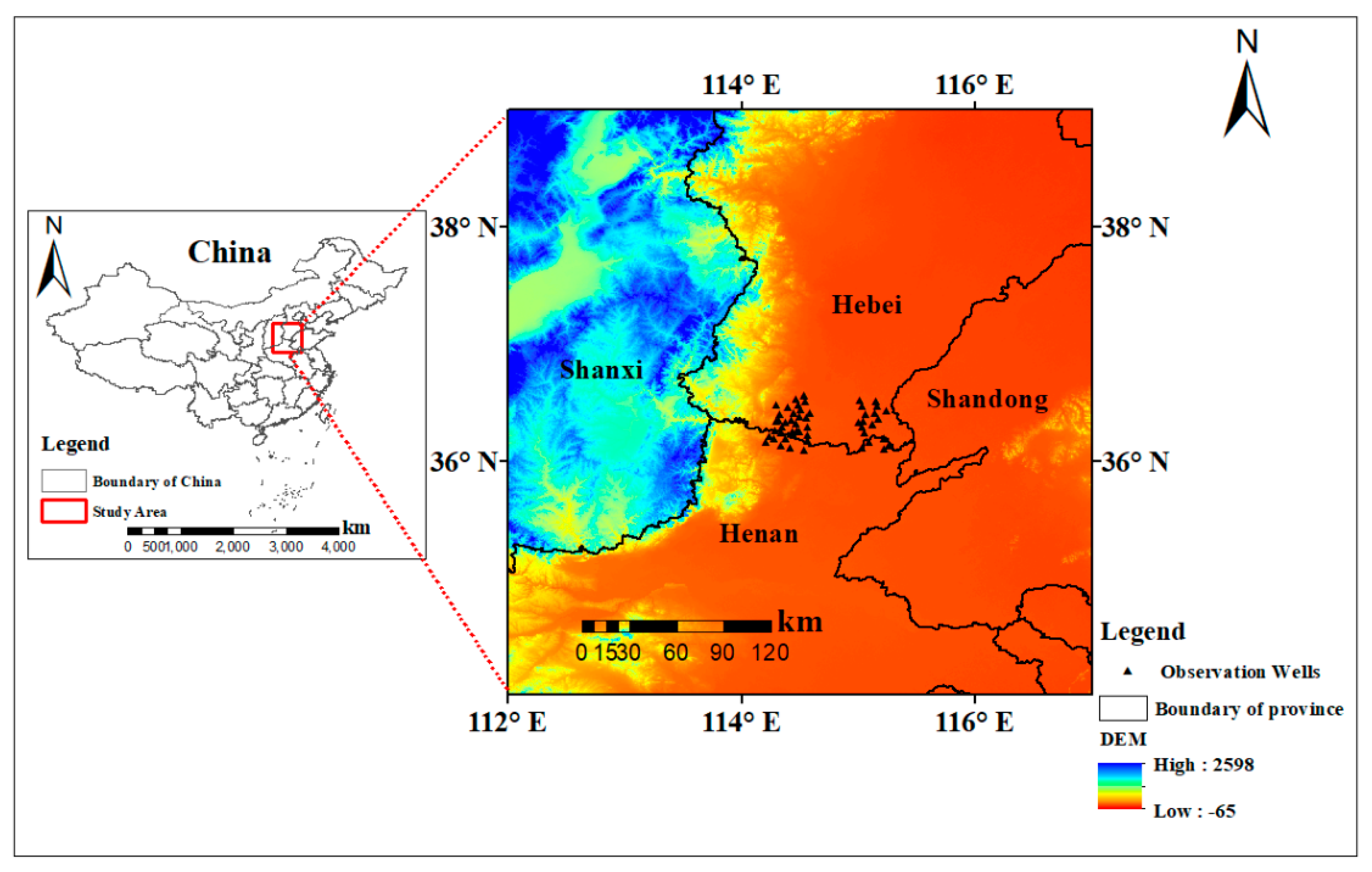
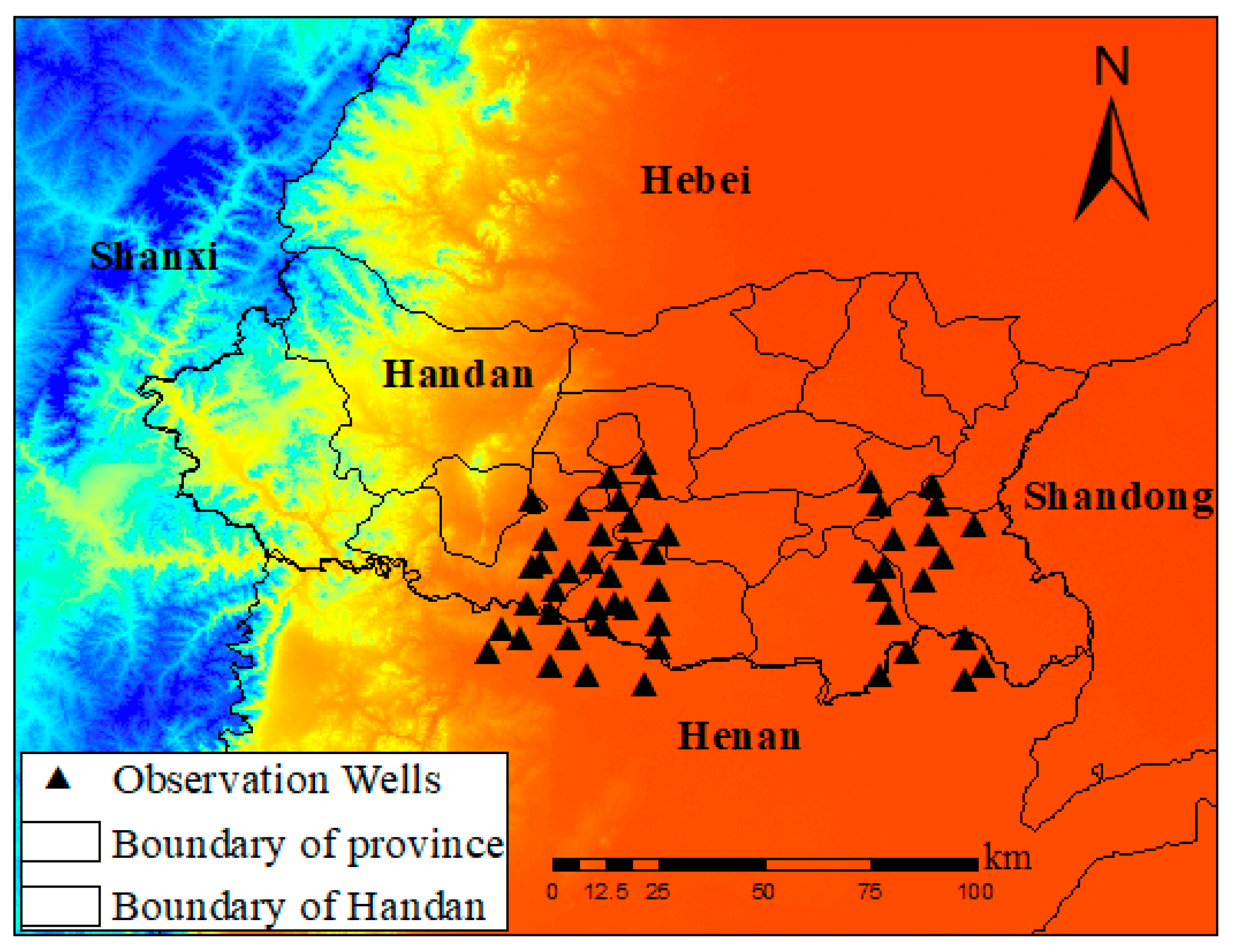
2.1. Study Area

The northeast of mainland China in the range of latitude and longitude between 34°N–39°N and 112°E–117°E was selected as the study area in this research, which includes Shanxi, Shandong, Henan, Hebei, Tianjin, Jiangsu, and Anhui provinces. The study area is densely populated and economically developed. It is one of China’s political, economic, and cultural prosperity. At the same time, the region also includes important grain production bases in China [43]. The terrain is relatively flat, with a general trend of gradual decline from west to east, which belongs to the boundary between temperate monsoon climate and subtropical monsoon climate. Mean annual temperature is between 8–15 ℃ and the mean precipitation is range from 500 to 600 mm. There is a prominent contradiction between water supply and demand in the study area [44,45]. Figure 1 shows the geographical location of the study area.

2.2. Data Source and Processing

There are mainly four sets of data in this study. The GRACE gravity satellite data provides the total water storage (TWS) and the groundwater storage (GWS), and the global land surface assimilation system (GLDAS) NOAH model data provides runoff, soil moisture, snow water equivalent, and canopy water data. The Global Land Evaporation Amsterdam Model (GLEAM) provides evapotranspiration data and TRMM 3B43 provides precipitation data. In the above data, the spatial resolution of GRACE data is 1°, while the other data all have a resolution of 0.25°, and the temporal resolution is monthly. The study period was 163 months from January 2003 to July 2016.

2.2.1. GRACE TWS

The GRACE satellite was launched on 17 March 2002, which is jointly implemented by NASA and DLR under the NASA Earth System Science Pathfinder Program [46,47]. It was designed to provide effective observation data for studying the changes in the Earth’s mass through high-precision time-varying gravitational fields [48,49,50]. There are three institutions that provide GRACE satellite data sets based on different algorithms, which are CSR (Center for Space Research, the University of Texas), GFZ (GeoForschungsZentrum Potsdam), and JPL (Jet Propulsion Laboratory), respectively [49,50]. GRACE data is divided into five different levels: Level-0, Level-1A, Level-1B, Level-2, and Level-3 [27]. In this research, we used level-three data provided by CSR [24] in the form of grid data product, which has undergone a series of processing, such as gaussian smoothing, destriping filter, glacier isostatic adjustment (GIA), and the anomalies relative has been deducted by default to 2004 to 2009 time-mean baseline. The total water storage should be multiplied the scaling factors to restore much of the energy removed by processing [30,37]. Total water storage of this product has a high accuracy and it is suitable to be applied in the research area of this study [49,51].

2.2.2. TRMM Precipitation

NASA and the Japanese space exploration agency (NASDA) developed the Tropical Rainfall Measuring Mission (TRMM). It is designed to measure rainfall in tropical and subtropical regions. It is the world’s first satellite equipped with rain measuring radar, which also carries microwave imager, visible light and infrared scanner, cloud and earth radiation energy system, and lightning imaging sensor [52]. This experiment adopted the TRMM 3B43 data products, and the data space coverage is 50°N–50°S in latitude, 180°W, and 180°E in longitude. The precipitation data were retrieved from Global Land Evaporation Amsterdam Model [53].

2.2.3. GLEAM Evaporation

GLEAM (Global Land Evaporation Amsterdam Model) was developed and provided by Miralles from the British Institute of Geographical Science at University of Bristol [54,55]. It is a set of algorithms that separately estimate the different components of land evaporation. The algorithm calculates five components of evapotranspiration (ET), including vegetation transpiration (ET), canopy interception evaporation (Ei), bare soil evaporation (Eb), snow sublimation evaporation (Es), and water surface evaporation (Ew). The spatial resolution is 0.25° × 0.25°, and the temporal resolution is divided into three types: day, month, and year, with the time span from 1980 to now. This study we select the monthly product data of v3.3a version, and this data were obtained from Global Land Evaporation Amsterdam Model [56].

2.2.4. GLDAS Data

The Goddard Space Flight Center (GSFC) provides Global Land Data Assimilation Systems (GLDAS) [57]. The GLDAS land surface assimilation system includes three land surface process models (CLM, Mosaic, NOAH) and a hydrological model (VIC), and it mainly includes two versions of data sets (GLDAS-1 and GLDAS-2). Among them, GLDAS-1 provides four sets of models to simulate global runoff, evapotranspiration, soil moisture, snow water equivalent, and canopy water, and other hydrological variables. The spatial resolution is 1° × 1°, the time resolution has 3 h and monthly scale, and the data set of NOAH model from 2000 to now is 0.25° × 0.25°. While GLDAS-2 only has NOAH model, provided data from 1948 to 2010, with spatial resolution of 1° × 1° and 0.25° × 0.25°. In this study, we mainly use the data of GLDAS-1 NOAH model with the 0.25° × 0.25° spatial resolution, which can be found in the Goddard Earth Sciences Data and Information Services Center (GES DISC) [58].

2.2.5. Ground-Based Measurements

In this study, the monthly groundwater level data of 57 observation wells in Handan, Hebei province from January 2006 to December 2015 were collected, which was provided by the groundwater monitoring bureau of Handan. These observation wells are densely distributed in Handan, so they can accurately verify the changes of underground water level in this area. Figure 2 shows the locations of observation wells.

2.3. Model Design

2.3.1. Random Forest Model

Breiman first proposed the Random Forest (RF) model in 2001 [38] as a new integrated machine learning method consisting of multiple classification and regression decision trees CART (Classification and Regression Trees) combination, which is mainly applied to regression and classification. The steps for modeling are as follows: firstly, in the original input data, the Bootstrap method was used to randomly extract multiple samples for training the model, and the unextracted data were used as data out of the bag to test the accuracy of the model. Subsequently, a decision tree is constructed for each training sample, and all of the sample decision trees are combined into random forest model. The RF results are the average of the prediction results of each decision tree. With its advantages in regression and classification, the RF model has been widely used in remote sensing and hydrology [32,59,60]. For a regression problem, the RF model has some unique advantages, as following: (1) it can input thousands of variables and it is not easy to overfitting; (2) it has high accuracy and it can run efficiently on large datasets; (3) it can detect the interaction and importance of variables; and, (4) it provided an effective method of estimating missing data and maintaining accuracy. The RF model has been widely used in established regression problem because of the above advantages, and good prediction results have been obtained [32].

2.3.2. Support Vector Machine Model

Vapnik originally proposed the Support Vector Machine (SVM) model [39] as a classification machine learning algorithm, which was later derived from regression algorithms. The theoretical basis is Vapnik Chervonenks Dimension (VC) and Structural Risk Minimized Inductive Principle. The optimization based on training error and minimizing the confidence range value can effectively solve the nonlinear regression problem. Jing et al. [56] described the details of the SVM method.

2.3.3. Artificial Neural Network

The artificial neural network (ANN) model [40] is a non-linear information processing system that is based on the abstraction, simplification, and simulation of the human brain, which is widely connected by a large number of neurons. ANN can realize multi-dimensional nonlinear precise mapping between the input layer and the output layer without setting up any mathematical calculation model between the two. In this study, we used a multi-layer feed-forward perceptron (MLP). A typical MLP consists of an input layer, an output layer, and one or more hidden layers. Each layer of MLP includes one or more neurons that are directionally linked to the neurons of the previous layer and the next layer.

2.3.4. Multiple Linear Regression

In a multi-factor geographic system, multiple (more than two) elements also have an interactive and interrelated linear regression relationship, which is called multiple linear regression (MLR). Nie et al. [61] found that some of the hydrological variables of GLDAS had a good linear relationship with the GRACE-derived TWS. Hence, in this study, we tried to use the MLR approach to compare the quality of the machine learning methods.

It is appropriate to select the random forest mode, given that the total storage is a complex hydrological variable, which is correlated with multiple variables, and that this study has a large number of training data.

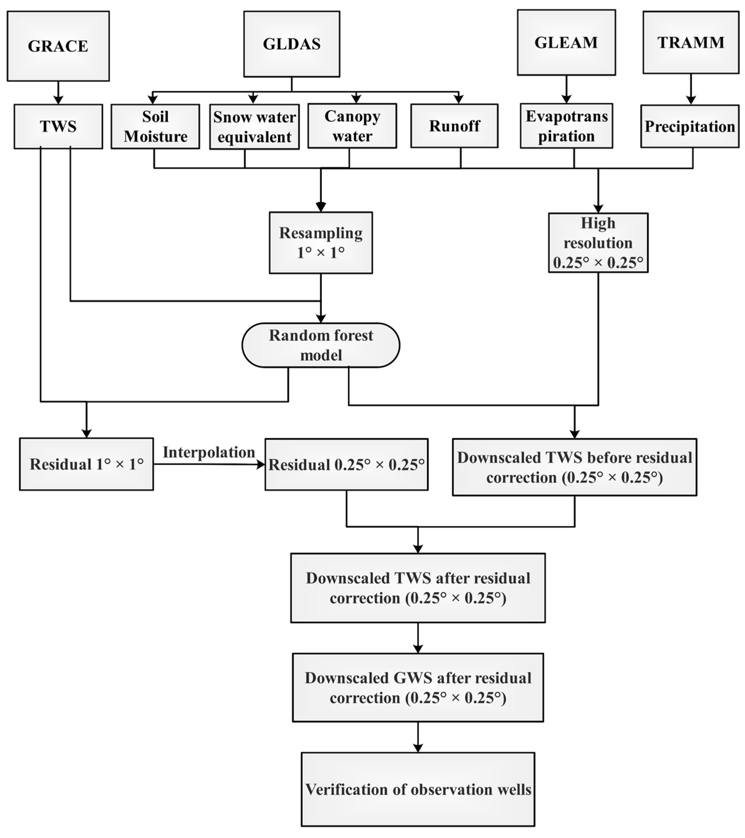
2.3.5. Downscaling Model Design

Random forest downscaling is a nonlinear statistical downscaling method. In this paper, we choose random forest model to downscale the TWS and GWS from 1° to 0.25°. The basic idea of th random forest downscaling model established the statistical relationship between TWS and hydrological variables (precipitation, evapotranspiration, runoff, soil moisture, snow water equivalent, and canopy water). We used the TWS as the dependent variable, and the hydrological variables as the independent variables. First, we established the relationship between TWS and hydrological variables at a spatial resolution of 1° and then applied it to the hydrological variables at a spatial resolution of 0.25° to obtain high resolution TWS. Figure 3 shows the flowchart of the downscaling process.

(1)

First, the six hydrological variables during January, 2003 to July, 2016 are resampled to 1°. Aggregate 0.25° precipitation, evapotranspiration, runoff, soil moisture, snow water equivalent, and canopy water monthly average value from 0.25° to 1° by pixel averaging, respectively. Subsequently, established the random forest model between TWS and six hydrological variables at a spatial resolution of 1°.

(2)

Secondly, the GRACE-derived TWS data subtracted the TWS of the RF model simulation in step (1) and then calculated the residual distribution of TWS at a spatial resolution of 1°, after which residual at 1° model is interpolated to 0.25° by cubic spline function [62].

(3)

Thirdly, the established RF model is applied to the hydrological variables at a spatial resolution of 0.25° to obtain the estimated 0.25° TWS of the RF model. Afterwards, the estimated TWS at 0.25° is added to the residual at 0.25° to obtain the monthly TWS data with a spatial resolution of 0.25° after a residual correction.

(4)

Finally, we might obtain the downscaling GWS by deducting soil moisture, snow water equivalent, and canopy water from GLDAS NOAH model with a spatial resolution of 0.25° from downscaling TWS. Subsequently, we verified the result with the measured water level data and the downscaling GWS.

2.4. Data Comparison and Error Analysis

In this paper, four indices are used to evaluate the downscaling TWS result. The testing data and its model prediction results are involved in the calculation. Correlation coefficient R, root mean square error (RMSE), Nash efficiency coefficient (NSE), and mean absolute error (MAE) are the four evaluation indices. The detailed description and calculation formula are as follows:

2.4.1. Correlation Coefficient (R)

The correlation coefficient refers to the degree of linear relationship between two variables. For the model construction, the higher the correlation coefficient R between validation data and simulation data, the better the model accuracy.

$$\mathrm{R}=\frac{{{\displaystyle \sum }}_{\mathrm{i}=1}^{\mathrm{N}}({\mathrm{X}}_{\mathrm{i}}-\overline{\mathrm{X}})({\mathrm{Y}}_{\mathrm{i}}-\overline{\mathrm{Y}})}{\sqrt{{{\displaystyle \sum }}_{\mathrm{i}=1}^{\mathrm{N}}{({\mathrm{X}}_{\mathrm{i}}-\overline{\mathrm{X}})}^2} \sqrt{{{\displaystyle \sum }}_{\mathrm{i}=1}^{\mathrm{N}}{({\mathrm{Y}}_{\mathrm{i}}-\overline{\mathrm{Y}})}^2}}$$

(1)

where Xi and Yi represent two independent data sets with the mean value of $\overline{\mathrm{X}}$ and $\overline{\mathrm{Y}}$. Xi represents the input total water storage, Yi represents the simulated value of RF model, and N is the total number of samples.

2.4.2. Root Mean Squared Error (RMSE)

Root-mean-square error is also called the standard error and it is the deviation between the real value and the predicted value of the model. The smaller the value, the closer the predicted value is to the real value, that is, the smaller the RMSE is, the higher the accuracy of the model.

$$\mathrm{RMSE}=\sqrt{\frac{{{\displaystyle \sum }}_{\mathrm{i}=1}^{\mathrm{N}}{({\mathrm{X}}_{\mathrm{i}}-{\mathrm{Y}}_{\mathrm{i}})}^2}{\mathrm{N}}}$$

(2)

2.4.3. Nash-Sutcliffe Efficiency Coefficient (NSE)

The Nash efficiency coefficient is generally used to test the estimated results of hydrological models, and in this paper, we used to test the accuracy of the random forest model. The value range of NSE is (−∞, 1). The closer NSE is to 1, the better the modeling accuracy and the higher the reliability of the model. The closer NSE is to 0, the closer the predicted value is to the average value of the real value, which means that the overall result is credible, but the process simulation error is relatively large. If NSE is much less than 0, then the model is less credible.

$$\mathrm{NSE}=1-\frac{{{\displaystyle \sum }}_{\mathrm{i}=1}^{\mathrm{N}}{({\mathrm{Y}}_{\mathrm{i}}-{\mathrm{X}}_{\mathrm{i}})}^2}{{{\displaystyle \sum }}_{\mathrm{i}=1}^{\mathrm{N}}{({\mathrm{X}}_{\mathrm{i}}-\overline{\mathrm{X}})}^2}$$

(3)

2.4.4. Mean Absolute Error (MAE)

The mean absolute error represents the average of the absolute value of the deviation of all single simulated values from the arithmetic mean, which can avoid the problem of the error canceling each other, so it can accurately reflect the actual prediction error.

$$\mathrm{MAE}=\frac{1}{\mathrm{N}}({\displaystyle \sum }_{\mathrm{i}=1}^{\mathrm{N}}\left|{\mathrm{Y}}_{\mathrm{i}}-{\mathrm{X}}_{\mathrm{i}}\right|)$$

(4)

2.5. Significance Test

In this study, we used the t-test as the significance test of the correlation between two data sets. At first, we should compute the correlation coefficient (R) of the time series and construct the hypothesis test. Finding a statistics book that has a table of critical values of R is the easiest way to test this hypothesis. The specified Significance level a is usually set at 0.05 (5%) or 0.01 (1%). We compare the threshold of correlation coefficient with the calculated correlation coefficient. The results can be divided into three situations: (1) |R| < R_0.05, v means that the correlation is not significant; (2) when R_0.05, v≤|, R| < R_0.01, v represents the level of correlation significant α = 0.05; and, (3) when |R|≥R_0.01, v represents a level of significant correlation α = 0.01.

3. Results

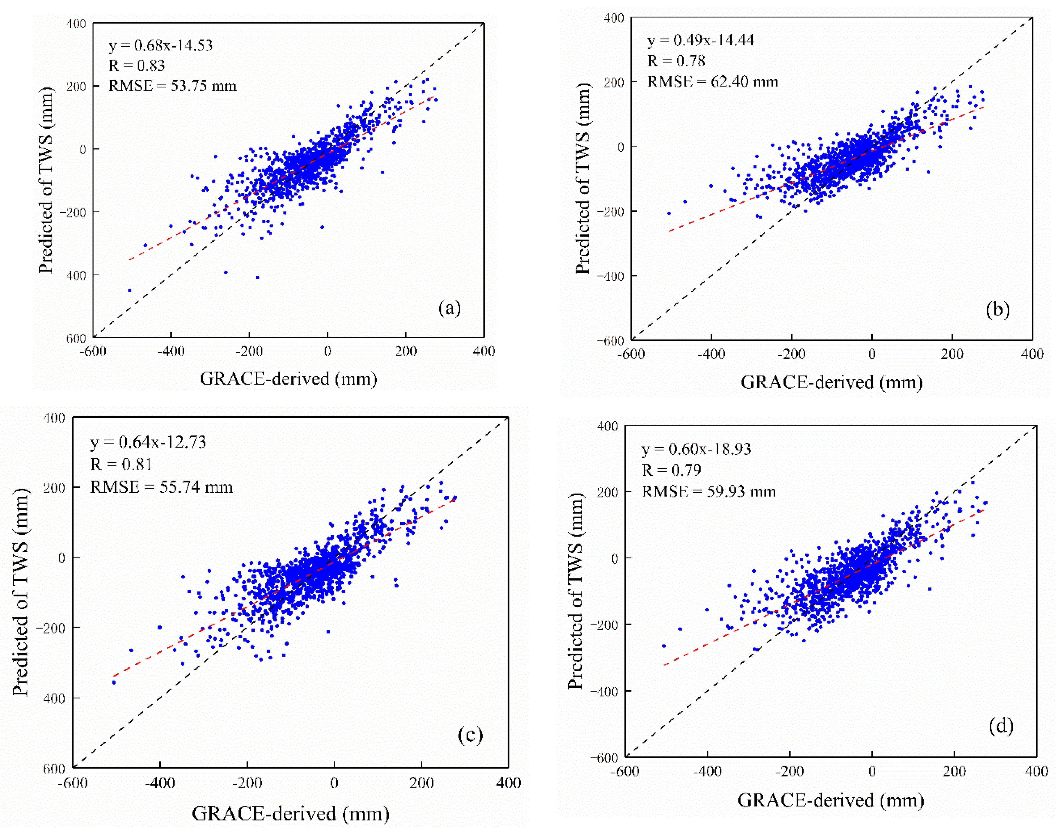
3.1. Accuracy Estimation of Random Forest Model

The original input data was divided into two parts by the method of random secondary sampling, in which 70% of the training data and the remaining 30% were taken as verification data, in order to verify the rationality of the random forest model. With the above six variables as input, four machine learning prediction models were established to predict the TWS. Figure 4 shows the comparison between the predicted results and the original GRACE-derived TWS.

In Figure 4, the x-coordinate represents the change value of GRACE-derived TWS in the verified data, and the y-coordinate represents the change value of predicted TWS after introducing the independent variable value of the verified data in the random forest model. From the scatter plots in Figure 4, the RF model has the highest correlation of 0.83 and the lowest RMSE of 53.75 mm, respectively, followed by the ANN model with the correlation coefficient of 0.81, slightly lower than the RF model. The results of the support vector machine and multiple linear regression are slightly worse. From

Table 1. Results of modeling accuracy of four machine learning methods.

Models	R	RMSE (mm)	MAE (mm)	NSE
RF	0.83	53.75	38.97	0.68
SVR	0.78	62.40	44.83	0.57
ANN	0.81	55.74	41.23	0.66
MLR	0.78	59.93	44.84	0.61

, the indicators of random forests are superior to other models, followed by artificial neural networks, and the results of SVR and MLR are poor. From the above results, it can be found the RF downscaling model is the best, which can meet the requirements of variable prediction. The predicted results, together with the residuals, can accurately predict high-resolution changes in TWS and GWS. Therefore, we only analyze the RF results in the following discussion.

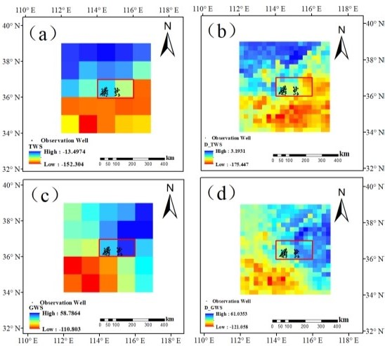
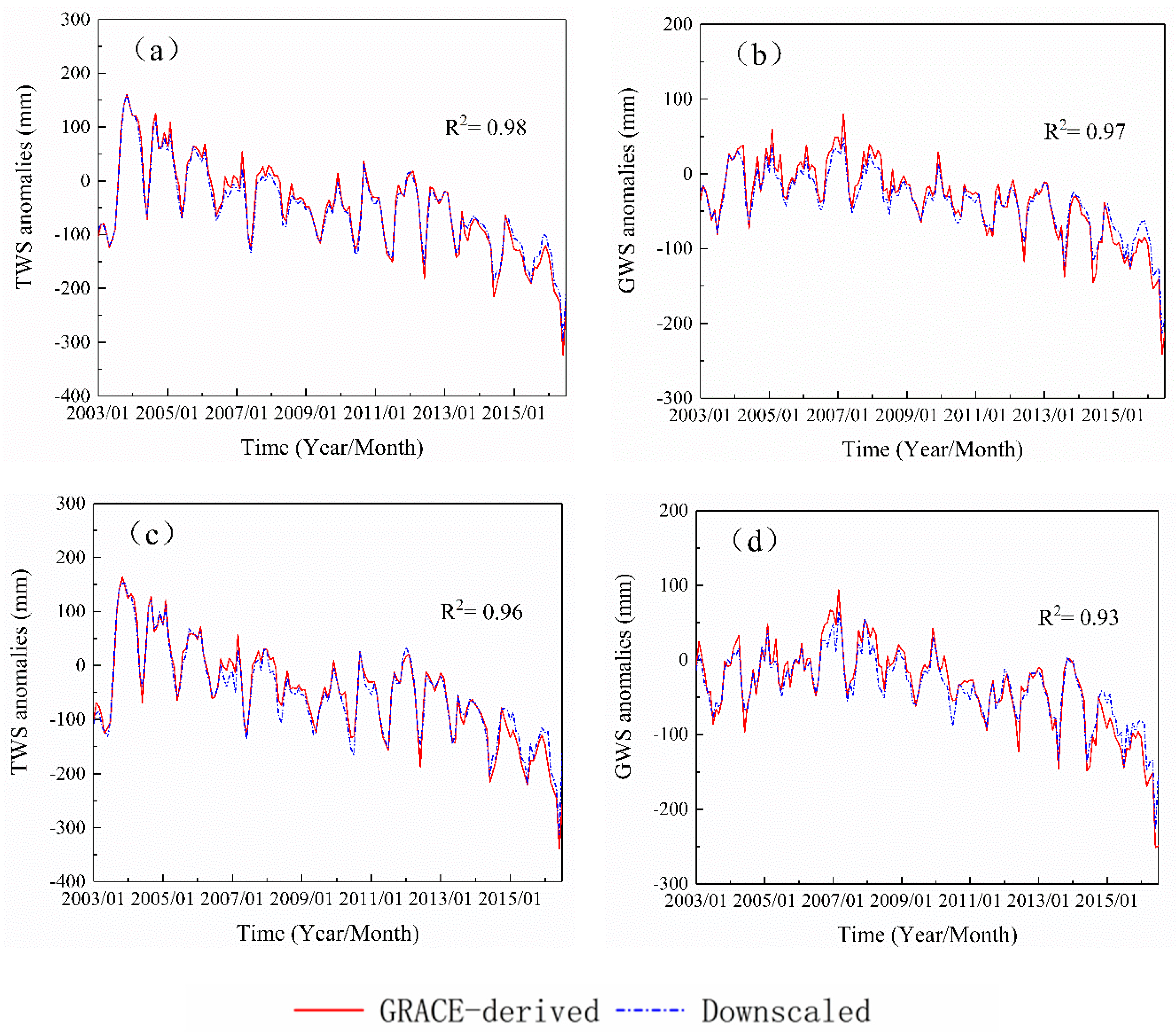
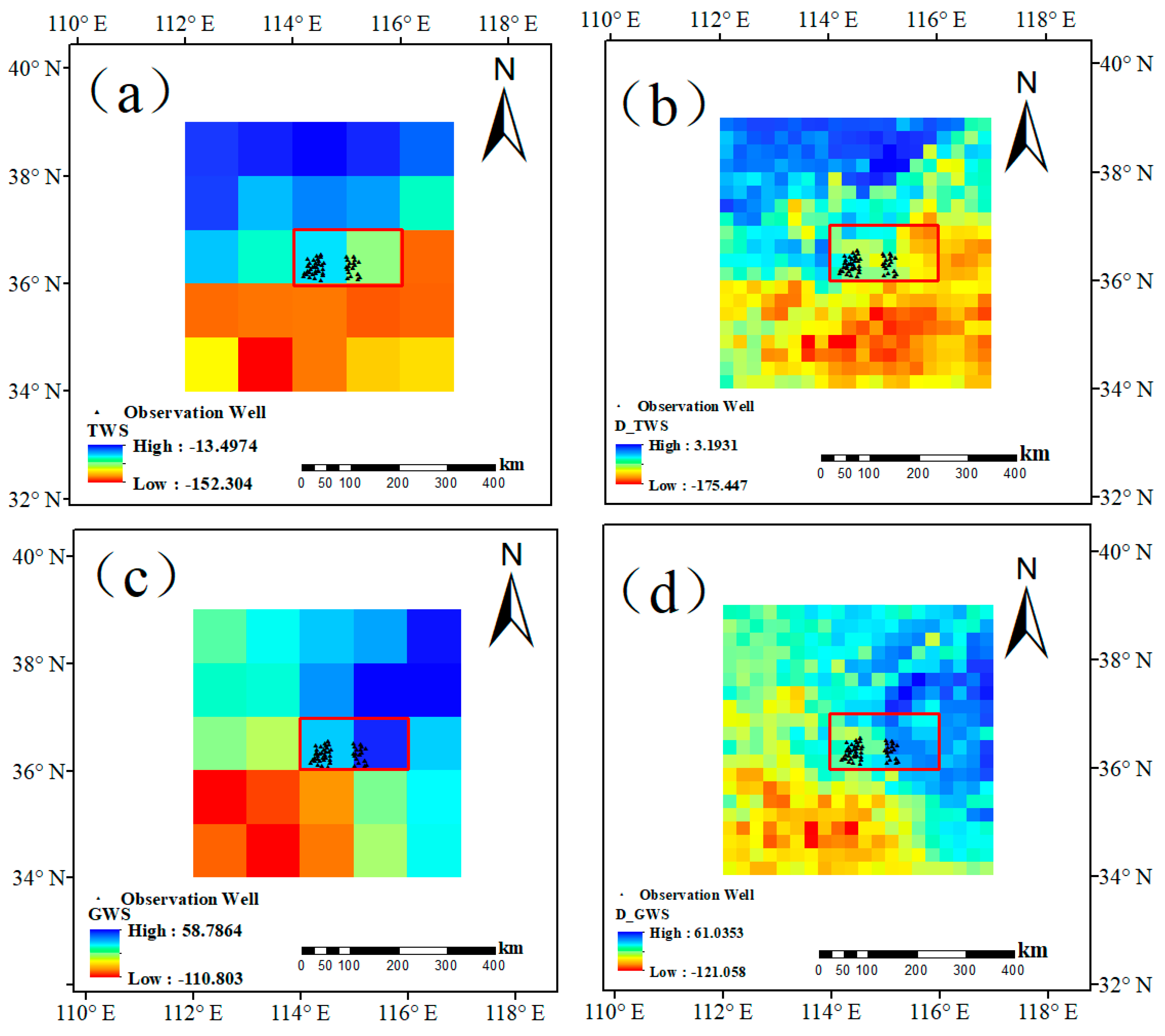
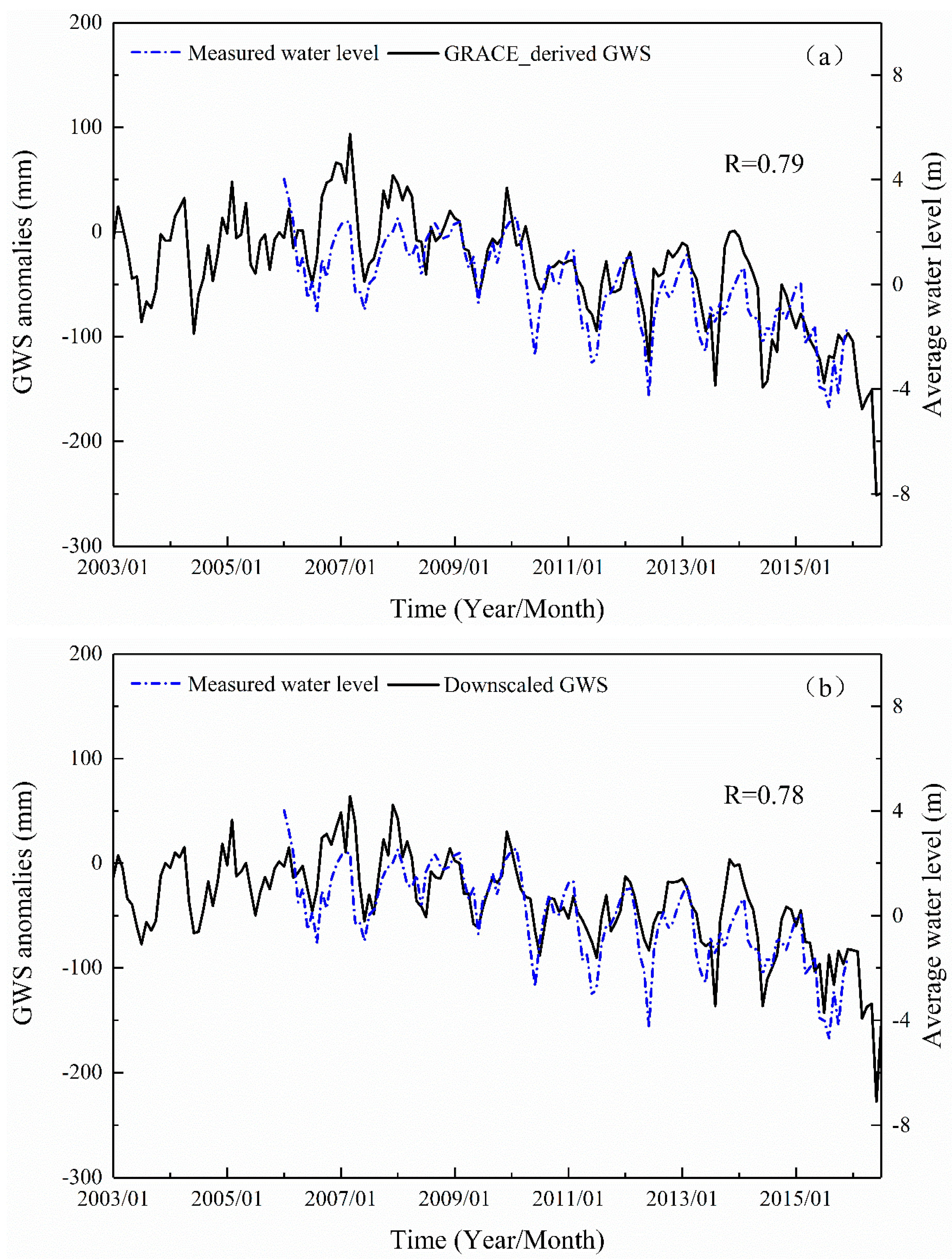
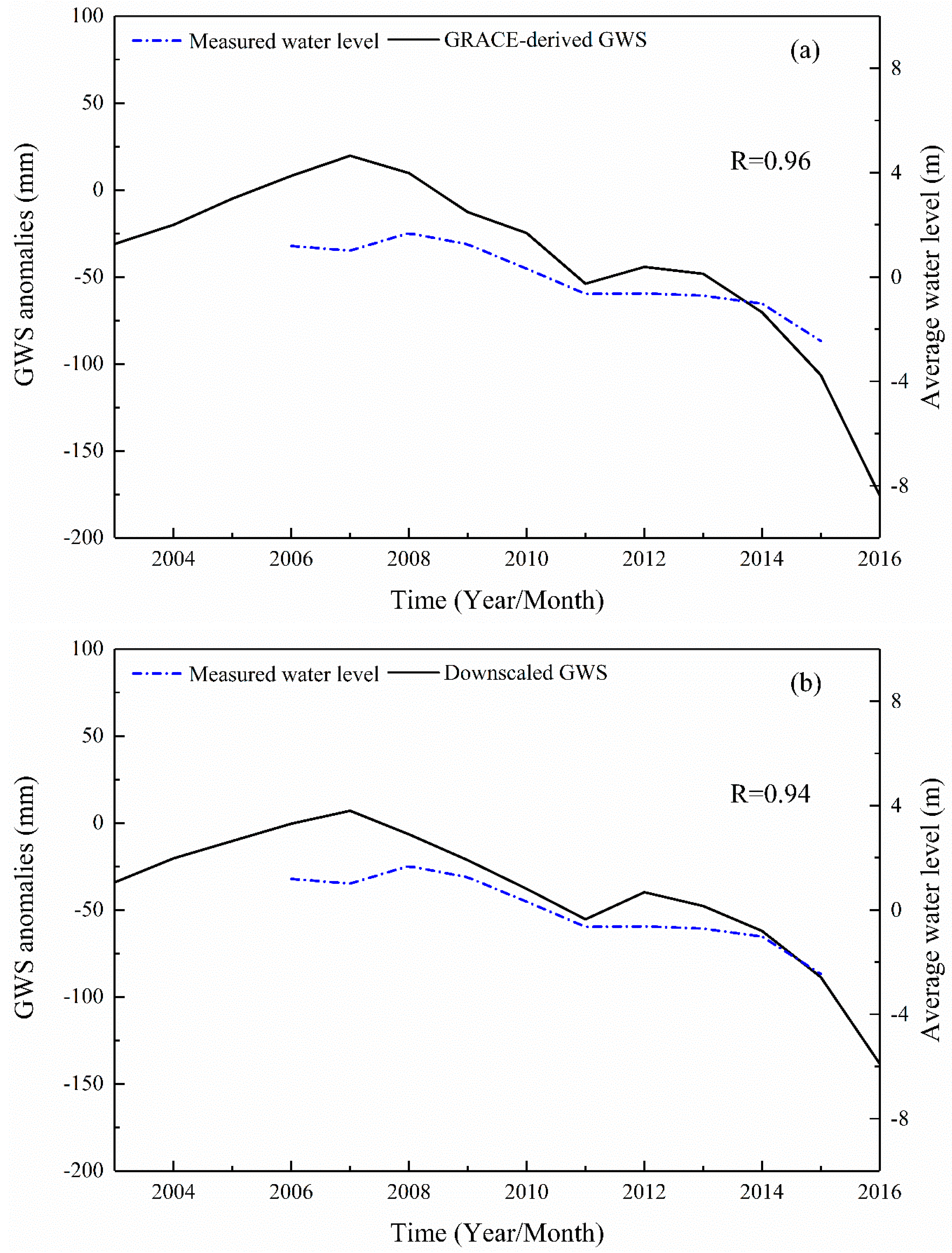
3.2. Time Series and Spatial Accuracy

The change trend of TWS and GWS in the study area is almost the same, and they are in a state of decline on the whole, which is consistent with the fact that GWS is the main component of TWS, which indicated that the results of TWS and GWS retrieved by GRACE are reliable. Figure 5 is the time series variation diagram of TWS GWS before and after downscaling, with spatial resolutions of 1° and 0.25°, respectively. It can be seen from the Figure 5 that the variation amplitude and value of TWS and GWS in the study area before and after downscaling are consistent, which indicated that the downscaling method based on random forest is reasonable in this study. Figure 5a shows the change of TWS in the whole study area before and after downscaling, with the correlation coefficient R² reaching 0.98. The fitting effect is the best. Figure 5b shows the change of GWS in the whole study area before and after downscaling, with the correlation coefficient R² reaching 0.97. Figure 5c shows the changes of TWS in the verified area in Handan, where there are 57 observations wells before and after downscaling, with the correlation coefficient R² reaching 0.96. Figure 5d shows the changes of GWS in the verified area in Handan, before and after downscaling, with the correlation coefficient R² reaching 0.93. In general, the downscaling result of TWS is better than that of GWS, which might be related to the direct downscaling result of TWS, while GWS are indirectly calculated. However, the downscaling results of random forests are credible from both the whole region and the local region. The spatial resolution after downscaling is higher and the spatial variation can be described in more detail.

We compared the spatial distribution of TWS and GWS before and after downscaling in order to analyze the consistency of spatial distribution before and after downscaling of the random forest model. As shown in Figure 6, we take the changes in TWS and GWS in February 2003 as an example. From the perspective of spatial variation, the TWS and GWS maintain good consistency both before and after downscaling. Among them, the TWS shows a decreasing trend from north to south. The region with the largest water storage is between 38° N and 39° N, and both of the images are obvious. The change of the maximum value before and after downscaling indicates that the downscaling TWS can more carefully depict their spatial changes. Similarly, the spatial variation trend of groundwater before and after downscaling is highly consistent. According to the above results, the downscaling method that is based on random forest model is effective.

We once again compared the interannual spatial variation rules of TWS and GWS, taking 2014 as an example to further illustrate the reliability of downscaling results, as shown in Figure 7. In 2014, the TWS and GWS in the study area showed similar changes on the whole in space, but there were also certain differences. It is embodied in the region from 34° N to 35° N, which might be related to the change of soil moisture water in this region. However, the spatial changes before and after downscaling are basically the same. It shows that the downscaling model that is constructed by random forest method is feasible, which can not only predict the change of water storage in the study area, but also depict the change trend of water storage with higher spatial resolution.

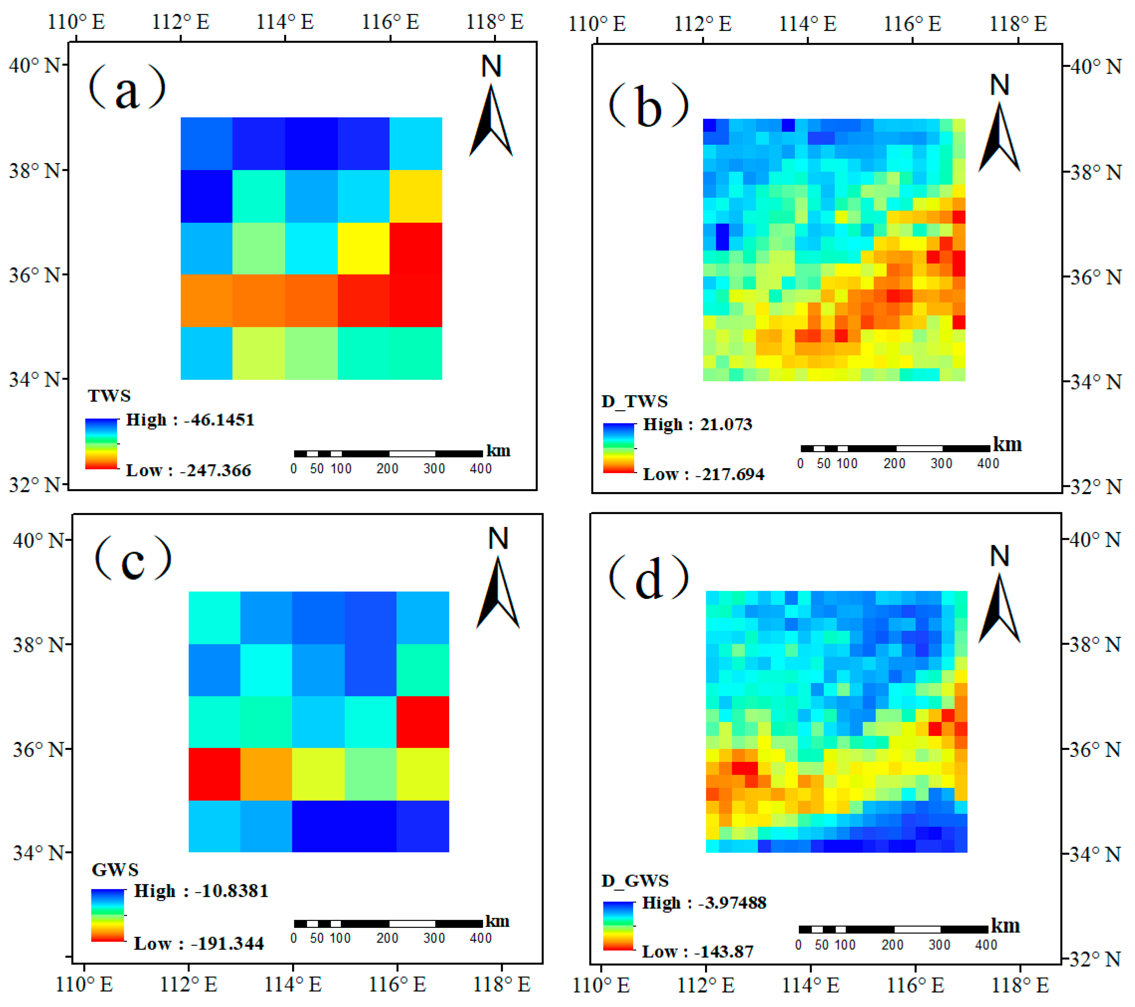
3.3. Testing and Spatial Accuracy

We compared the measured water level with the GRACE-derived GWS and the downscaling GWS in order to further explore the reliability of downscaling results. With the correlation coefficient R as the criterion, the higher R is, the more accurate the result of downscaling. Figure 8 and Figure 9 show the correlation between the measured water level and GWS in Handan area. The verified data are, respectively, the average of 57 measured sites on the monthly scale, the average of the GRACE-derived GWS, and the downscaling GWS in the grid (as shown in Figure 6 the inner region of the red rectangle). The results show that, on the monthly scale, the correlation between downscaling results and measured water level is 0.78, and on the annual scale is 0.94, both of which reach the confidence level of 0.01. The correlation coefficients between GRACE-derived GWS and measured water level are 0.79 and 0.96, respectively. Therefore, the random forest downscaling model not only improves the spatial resolution of data, but also ensures the accuracy of data.

4. Discussion

Overall, high-resolution hydrological products are a hot topic in future research. We have downscaled GWS from 1° to 0.25° based on the downscaling model of random forest, which provided a possibility for further research on GRACE data. The results showed that the RF downscaling model could be well applied to the study area. The verification results of groundwater level data of only 57 observation wells were used in this study due to the limitation of the measured data. The observation wells were distributed in two grids, weakening the effect of spatial heterogeneity and making the verification results more reliable. If we could get more measured data, then the results might be more reliable. Handan is located in the southern part of Hebei Province, and its topography descends stepwise from west to east, and the landform types are complex and diverse. It belongs to the East Asian monsoon climate zone and it is a continental monsoon climate that transitions from warm temperate semi-humid regions to semi-arid regions. From the verification results, the RF downscaling model is suitable for continental monsoon climate zone, but whether this method is applicable to other climatic regions needs further study. However, in this study, we have provided suitability of RF method in downscaling TWS and GWS, which could be used in other regions.

The use of satellite data can improve the applicability of data-scarce areas with limited hydrological variables, such as groundwater observation well data with uneven spatial and temporal distribution. However, these data sources also bring significant uncertainty. For example, GRACE data has its own uncertainty in data processing, and other input data has contributed to uncertainty and potential error propagation of the total input data [30]. In this research, we chose CSR level-three data products. We multiplied scaling coefficients at 1° location to restore much of the energy removed by the destriping, gaussian, and degree 60 filters to the land grids, but it may be uncertain in hydrology models at inter-annual. In subsequent research, readers can choose different data, such as using an advanced mass concentration (‘mascon’) data [63] and comparing the results of multiple data to reduce data uncertainty. At the same time, unavoidable systematic uncertainty in the training models of machine learning still remains. We compare the results of several common machine learning models (e.g., RF model, MLR model, SVR model, and ANN model). From the results, it can be found that the result of RF model is best. It shows that the random forest model is not easy overfitting and noise immunity ability is better than other machine learning models. When compared with other machine learning models, the RF downscaling model mitigated these errors, because it can handle errors associated with input data.

The advantage of the RF downscaling model is that we can simultaneously input multiple variables, which increases the flexibility of the model. At the same time, the input variables are independent of each other in the model and we can select different variable factors of the different study area. From the view of regional water management, they pay more attention to water storage at small regional scales than the water storage of GRACE-derived, and the downscaling random forest model can effectively solve the problem of current coarse resolution data, which provide more detailed information for water decision makers. The results of random forests are the best in the four machine learning downscaling models, followed by artificial neural networks. The worst result of the support vector machine might be that the data anti-noise effect of the model is not as good as the firs at two. Therefore, the reader can further experiment in the RF model and the ANN model; at the same time, I think that the method can be improved in the following aspects in the future study:

(1)

Syed et al. [12] pointed out that the zonal average indicates that precipitation in the tropics dominates the TWSC, evapotranspiration is the most effective in the mid-latitudes, and snowmelt runoff is the main dissipation flux in the high latitudes. Therefore, in subsequent experiments, according to the latitude of the study area, remote sensing products with higher precision and finer resolution can be selected for research, and the impact of local economic and demographic conditions on water reserves needs to be properly considered.

(2)

From the global perspective, it can be divided into arid regions, semi-arid regions, and humid regions. According to the different characteristics of the study area, other variables, such as temperature, NDVI, DEM, and so on, can be appropriately added.

(3)

For regional scale research, we can select higher resolution remote sensing products to meet the requirements of regional water managers.

5. Conclusions

With the launch and application of GRACE gravity satellite, it provides a new research method for exploring large-scale groundwater changes. However, with the progress of human society, the change of low-resolution water storage is increasingly difficult to meet people’s requirements and demand. The need for detailed changes in groundwater is becoming more and more urgent. In this study, we tried to use four common machine learning methods to conduct downscaling study. From the results, the RF downscaling model has the highest accuracy, and the ANN model is second. Therefore, we proposed a downscaling method that was based on random forest to comprehensively consider the influence of multiple hydrological variables on TWS. We successfully downscaled the TWS from 1° to 0.25° and calculated the high-resolution GWS.

From the perspective of long time series, this downscaling method could predict the changes of regional water storage well. In both the whole study region and in the small local area, the prediction results of the model are ideal. The error downscaling result is very small, and the amplitude and phase of water storage before and after downscaling is consistent. From the perspective of spatial variation, the downscaling data can effectively capture the subgrid heterogeneity of TWS and GWS, which cannot be realized in the original scale. In addition, the method has a low cost and it can be easily used to detect changes in local and small water storage.

From the verification results of measured water level, the measured groundwater level data is in good agreement with the downscaling groundwater data. On the monthly and annual scales, the correlation coefficients reached 0.78 and 0.93, respectively, and they passed the confidence level of 0.01, where it is 0.79 and 0.96 before downscaling. It is shown that the method can not only improve the spatial resolution of the data effectively, but also ensure the accuracy of the data.

References

1. Rodell, M.; Velicogna, I.; Famiglietti, J.S. Satellite-based estimates of groundwater depletion in India. Nature 2009, 460, 999. [Google Scholar] [CrossRef] [PubMed] [Green Version]
2. Wang, Y. The Evaluation of Environmental Quality of Groundwater in Inland Plains—A Study on Yanqi County in Xinjiang. Master’s Thesis, Xinjiang Agricultural University, Urumqi, China, 2010. [Google Scholar]
3. Famiglietti, J.S.; Lo, M.; Ho, S.L.; Bethune, J.; Anderson, K.J.; Syed, T.H.; Swenson, S.C.; de Linage, C.R.; Rodell, M. Satellites measure recent rates of groundwater depletion in California’s Central Valley. Geophys. Res. Lett. 2011, 38. [Google Scholar] [CrossRef] [Green Version]
4. Long, D.; Chen, X.; Scanlon, B.R.; Wada, Y.; Hong, Y.; Singh, V.P.; Chen, Y.; Wang, C.; Han, Z.; Yang, W. Have GRACE satellites overestimated groundwater depletion in the Northwest India Aquifer? Sci. Rep. 2016, 6, 24398. [Google Scholar] [CrossRef] [PubMed]
5. Ye, S.H.; Huang, C. Space technique monitoring and prediction of ground water chinges. Prog. Geophys. 2007, 4, 1030–1034. (In Chinese) [Google Scholar]
6. Ramilliena, G.; Frapparta, F.; Cazenavea, A.; Güntnerb, A. Time variations of land water storage from an inversion of 2 years of GRACE Geoids. Erath Planet. Sci. Lett. 2005, 235, 283–301. [Google Scholar] [CrossRef] [Green Version]
7. Castellazzi, P.; Longuevergne, L.; Martel, R.; Rivera, A.; Brouard, C.; Chaussard, E. Quantitative mapping of groundwater depletion at the water management scale using a combined GRACE/InSAR approach. Remote Sens. Environ. 2018, 205, 408–418. [Google Scholar] [CrossRef]
8. Davis, J.L.; Elósegui, P.; Mitrovica, J.X. Climate-driven deformation of the solid Earth from GRACE and GPS. Geophys. Res. Lett. 2004, 31, 357–370. [Google Scholar] [CrossRef] [Green Version]
9. Yeh, P.J.F.; Swenson, S.C.; Famiglietti, J.S.; Rodell, M. Remote sensing of groundwater storage changes in Illinois using the Gravity Recovery and Climate Experiment (GRACE). Water Resour. Res. 2006, 42. [Google Scholar] [CrossRef]
10. Feng, W.; Zhong, M.; Lemoine, J.; Biancale, R.; Hsu, H.; Xia, J. Evaluation of groundwater depletion in North China using the Gravity Recovery and Climate Experiment (GRACE) data and ground-based measurements. Water Resour. Res. 2013, 49, 2110–2118. [Google Scholar] [CrossRef]
11. Rodell, M.; Chen, J.; Kato, H.; Famiglietti, J.S.; Nigro, J.; Wilson, C.R. Estimating groundwater storage changes in the Mississippi River basin (USA) using GRACE. Hydrogeol. J. 2007, 15, 159–166. [Google Scholar] [CrossRef]
12. Syed, T.H.; Famiglietti, J.S.; Rodell, M.; Chen, J.; Wilson, C.R. Analysis of terrestrial water storage changes from GRACE and GLDAS. Water Resour. Res. 2008, 44. [Google Scholar] [CrossRef]
13. Velicogna, I.; Wahr, J. Greenland mass balance from GRACE. Geophys. Res. Lett. 2005, 32. [Google Scholar] [CrossRef] [Green Version]
14. Frappart, F.; Papa, F.; Famiglietti, J.S.; Prigent, C.; Rossow, W.B.; Seyler, F. Interannual variations of river water storage from a multiple satellite approach: A case study for the Rio Negro River basin. J. Geophys. Res. Atmos. 2008, 113. [Google Scholar] [CrossRef] [Green Version]
15. Zhong, M.; Duan, J.; Xu, H.; Pen, P.; Yan, H.; Zhu, Y. Satellite gravity observation was used to study the change trend of medium and long space scale of China’s land water in recent 5 years. Chin. Sci. Bull. 2009, 54, 1290–1294. (In Chinese) [Google Scholar]
16. Long, D.; Yang, Y.; Wada, Y.; Hong, Y.; Liang, W.; Chen, Y. Deriving scaling factors using a global hydrological model to restore GRACE total water storage changes for China’s Yangtze River Basin. Remote Sens. Environ. 2015, 168, 177–193. [Google Scholar] [CrossRef]
17. Rodell, M.; Famiglietti, J.S.; Wiese, D.N.; Reager, J.T.; Beaudoing, H.K.; Landerer, F.W.; Lo, M.H. Emerging trends in global freshwater availability (vol 557, pg 651, 2018). Nature 2019, 565, E7. [Google Scholar] [CrossRef]
18. Swenson, S.; Wahr, J.; Milly, P.C.D. Estimated accuracies of regional water storage variations inferred from the Gravity Recovery and Climate Experiment (GRACE). Water Resour. Res. 2003, 39, 1121–1134. [Google Scholar] [CrossRef]
19. Richey, A.S.; Thomas, B.F.; Lo, M.; Reager, J.T.; Famiglietti, J.S.; Voss, K.; Swenson, S.; Rodell, M. Quantifying renewable groundwater stress with GRACE. Water Resour. Res. 2015, 52, 4184–4187. [Google Scholar] [CrossRef]
20. Feng, W.; Wang, C.; Mu, D.; Zhong, M.; Zhong, Y.; Xu, H. Groundwater storage variations in the North China Plain from GRACE with spatial constraints. Chin. J. Geophys. 2017, 60, 1630–1642. (In Chinese) [Google Scholar]
21. Ran, Q.; Pan, Y.; Wang, Y.R.; Chen, L.H.; Xu, H.L. Estimation of annual groundwater exploitation in Haihe River Basin by use of GRACE satellite data. Adv. Sci. Technol. Water Res. 2013, 33, 42–46. (In Chinese) [Google Scholar]
22. Scanlon, B.R.; Longuevergne, L.; Long, D. Ground referencing GRACE satellite estimates of groundwater storage changes in the California Central Valley, USA. Water Resour. Res. 2012, 48, W04520. [Google Scholar] [CrossRef] [Green Version]
23. Alley, W.M.; Konikow, L.F. Bringing GRACE Down to Earth. Ground Water 2015, 53, 826–829. [Google Scholar] [CrossRef] [PubMed]
24. Miro, M.E.; Famiglietti, J.S. Downscaling GRACE Remote Sensing Datasets to High-Resolution Groundwater Storage Change Maps of California’s Central Valley. Remote Sens. 2018, 10, 143. [Google Scholar] [CrossRef] [Green Version]
25. Liu, C.M.; Liu, W.B.; Fu, G.B.; OuYang, R.L. A discussion of some aspects of statistical downscaling in climate impacts assessment. Adv. Water Sci. 2012, 23, 427–437. (In Chinese) [Google Scholar]
26. Zhang, M.Y.; Peng, D.Z.; Hu, L.J. Research Progress on Statistical Downscaling Methods. South-to-North South-to-North Water Transf. Water Sci. Technol. 2013, 11, 118–122. (In Chinese) [Google Scholar]
27. Liu, Y.H.; Guo, W.D.; Feng, J.M.; Zhang, K.X. A Summary of Methods for Statistical Downscaling of Meteorological Data. Adv. Earth Sci. 2011, 26, 837–847. (In Chinese) [Google Scholar]
28. Ning, S.W.; Ishidaira, H.; Wang, J. Statistical downscaling of GRACE-derived terrestrial water storage using satellite and GLDAS products. J. Jpn. Soc. Civ. Eng. 2014, 70, 133–138. [Google Scholar] [CrossRef]
29. Yin, W.; Hu, L.; Zhang, M.; Wang, J.; Han, S. Statistical Downscaling of GRACE-Derived Groundwater Storage Using ET Data in the North China Plain. J. Geophys. Res. Atmos. 2018, 123, 5973–5987. [Google Scholar] [CrossRef]
30. Seyoum, W.M.; Kwon, D.; Milewski, A.M. Downscaling GRACE TWSA Data into High-Resolution Groundwater Level Anomaly Using Machine Learning-Based Models in a Glacial Aquifer System. Remote Sens. 2019, 11, 824. [Google Scholar] [CrossRef] [Green Version]
31. Sun, A.Y. Predicting groundwater level changes using GRACE data. Water Resour. Res. 2013, 49, 5900–5912. [Google Scholar] [CrossRef]
32. Chen, S.; She, D.; Zhang, L.; Guo, M.; Liu, X. Spatial Downscaling Methods of Soil Moisture Based on Multisource Remote Sensing Data and Its Application. Water-Sui. 2019, 11, 1401. [Google Scholar] [CrossRef] [Green Version]
33. Li, W.; Ni, L.; Li, Z.; Duan, S.; Wu, H. Evaluation of Machine Learning Algorithms in Spatial Downscaling of MODIS Land Surface Temperature. IEEE J. Sel. Top. Appl. Earth. Obs. Remote. Sens. 2019, 12, 2299–2307. [Google Scholar] [CrossRef]
34. Shi, Y.; Song, L.; Xia, Z.; Lin, Y.; Myneni, R.B.; Choi, S.; Wang, L.; Ni, X.; Lao, C.; Yang, F. Mapping Annual Precipitation across Mainland China in the Period 2001–2010 from TRMM3B43 Product Using Spatial Downscaling Approach. Remote Sens. 2015, 7, 5849–5878. [Google Scholar] [CrossRef] [Green Version]
35. Li, B.; Rodell, M.; Zaitchik, B.F.; Reichle, R.H.; Koster, R.D.; van Dam, T.M. Assimilation of GRACE terrestrial water storage into a land surface model: Evaluation and potential value for drought monitoring in western and central Europe. J. Hydrol. 2012, 446, 103–115. [Google Scholar] [CrossRef] [Green Version]
36. Schmidt, R.; Schwintzer, P.; Flechtner, F.; Reigber, C.; Guntner, A.; Doll, P.; Ramillien, G.; Cazenave, A.; Petrovic, S.; Jochmann, H.; et al. GRACE observations of changes in continental water storage. Glob. Planet. Chang. 2006, 50, 112–126. [Google Scholar] [CrossRef]
37. Yang, P.; Xia, J.; Zhan, C.; Wang, T. Reconstruction of terrestrial water storage anomalies in Northwest China during 1948–2002 using GRACE and GLDAS products. Hydrol. Res. 2018, 49, 1594–1607. [Google Scholar] [CrossRef] [Green Version]
38. Breiman, L. Random Forest. Mach. Learn. 2001, 45, 5–32. [Google Scholar] [CrossRef] [Green Version]
39. Vapnik, V.N. Statistical Learning Theory; Wiley: New York, NY, USA, 1998. [Google Scholar]
40. Ghorbani, M.A.; Khatibi, R.; Hosseini, B.; Bilgili, M. Relative importance of parameters affecting wind speed prediction using artificial neural networks. Theor. Appl. Climatol. 2013, 114, 107–114. [Google Scholar] [CrossRef]
41. Wang, J.; Zhang, J.M.; Ning, S.W.; Wang, H. Downscaling Analysis of GRACE Terrestrial Water Storage Changes in Yunnan Province. Water Res. Power 2018, 36, 1–5. (In Chinese) [Google Scholar]
42. Wang, S.Q.; Song, X.F.; Wang, Q.X.; Xiao, Q.G.; Liu, C.M. Dynamic Features of Shallow Groundwater in North China Plain. Acta Geogr. Sin. 2008, 63, 435–445. (In Chinese) [Google Scholar]
43. Cao, G.; Scanlon, B.R.; Han, D.; Zheng, C. Impacts of thicken in gun saturated zone on groundwater recharge in the North China Plain. J. Hydrol. 2016, 537, 260–270. [Google Scholar] [CrossRef]
44. Wang, S.; Shao, J.; Song, X.; Zhang, Y.; Huo, Z.; Zhou, X. Application of MODFLOW and geographic information system to groundwater flow simulation in North China Plain. China. Environ. Geol. 2008, 55, 1449–1462. [Google Scholar] [CrossRef]
45. Guo, H.; Zhang, Z.; Cheng, G.; Li, W.; Li, T.; Jiao, J.J. Groundwater-derived land subsidence in the North China Plain. Environ. Earth Sci. 2015, 74, 1415–1427. [Google Scholar] [CrossRef]
46. Feng, W. GRAMAT: a comprehensive Matlab toolbox for estimating global mass variations from GRACE satellite data. Earth Sci. Inform. 2019, 12, 389–404. [Google Scholar] [CrossRef]
47. Thomas, A.C.; Reager, J.T.; Famiglietti, J.S.; Rodell, M. A grace-based water storage deficit approach for hydrological drought characterization. Geophys. Res. Lett. 2014, 41, 1537–1545. [Google Scholar] [CrossRef] [Green Version]
48. Wang, D.; Zhang, G. Groundwater Ensure Capacity Spatial-temporal Characteristics and Mechanism in Main Grain Producing. Acta Geoscientica Sinica. 2017, 38, 47–50. (In Chinese) [Google Scholar]
49. Landerer, F.W.; Swenson, S.C. Accuracy of scaled GRACE terrestrial water storage estimates. Water Resour. Res. 2012, 48, W04531. [Google Scholar] [CrossRef]
50. Wahr, J.; Molenaar, M.; Bryan, F. Time variability of the Earth’s gravity field: Hydrological and oceanic effects and their possible detection using GRACE. J. Geophys. Res. Solid Earth 1998, 103, 30205–30229. [Google Scholar] [CrossRef]
51. Seyoum, W.M.; Milewski, A.M. Improved methods for estimating local terrestrial water dynamics from grace in the northern high plains. Adv. Water Resour. Res. 2017, 110, 279–290. [Google Scholar] [CrossRef]
52. Kummerow, C.; Simpson, J.; Thiele, O.; Barnes, W.; Chang, A.; Stocker, E.; Adler, R.F.; Hou, A.; Kakar, R.; Wentz, F.; et al. The status of the Tropical Rainfall Measuring Mission (TRMM) after two years in orbit. J. Appl. Meteorol. 2000, 39, 1965–1982. [Google Scholar] [CrossRef]
53. Sciences Data and Information Services Center (GES DISC). TRMM_3B43: TRMM (TMPA/3B43) Rainfall Estimate L3 1 Month 0.25 Degree × 0.25 Degree V7. Available online: https://disc.gsfc.nasa.gov/datasets/TRMM_3B43_7/summary?keywords=TRMM (accessed on 24 July 2019).
54. Miralles, D.G.; Holmes, T.R.H.; Jeu, R.A.M. Global land-surface evaporation estimated from satellite-based observations. Hydrol. Earth Syst. Sci. 2010, 7, 8479–8519. [Google Scholar] [CrossRef] [Green Version]
55. Martens, B.; Miralles, D.G.; Lievens, H.; van der Schalie, R.; de Jeu, R.A.M.; Fernandez-Prieto, D.; Beck, H.E.; Dorigo, W.; Verhoest, N. GLEAM v3: Satellite-based land evaporation and root-zone soil moisture. Geosci. Model Dev. 2017, 10, 1903–1925. [Google Scholar] [CrossRef] [Green Version]
56. Global Land Evaporation Amsterdam Model (GLEAM). Version 3.3a Datasets. Available online: https://www.gleam.eu (accessed on 24 May 2019).
57. Rodell, M.; Houser, P.R.; Jambor, U.; Gottschalck, J.; Mitchell, K.; Meng, C.J. The global land data assimilation system. Bull. Am. Meteorol. Soc. 2004, 85, 381–394. [Google Scholar] [CrossRef] [Green Version]
58. Global Land Data Assimilation Systems (GLDAS). Goddard Earth Sciences Data and Information Services Center (GES DISC). Available online: https://disc.gsfc.nasa.gov/datasets (accessed on 24 July 2019).
59. Jing, W.; Yang, Y.; Yue, X.; Zhao, X. A Comparison of Different Regression Algorithms for Downscaling Monthly Satellite-Based Precipitation over North China. Remote Sens. 2016, 8, 835. [Google Scholar] [CrossRef] [Green Version]
60. Junwei, H.; Shanyou, Z.; Guixin, Z. Downscaling land surface temperature based on random forest algorithm. Remote Sens. Land Res. 2018, 30, 78–86. [Google Scholar]
61. Nie, N.; Zhang, W.C.; Zhang, Z.J.; Guo, H.D.; Ishwaran, N. Reconstructed terrestrial water storage change (ΔTWS) from 1948 to 2012 over the Amazon Basin with the latest GRACE and GLDAS products. Water Resour. Manag. 2016, 30, 279–294. [Google Scholar] [CrossRef]
62. Guler, H.G.; Baykal, C.; Ozyurt, G.; Kisacik, D. Performance of Statistical Temporal Downscaling Techniques of Wind Speed Data over Aegean Sea; European Geosciences Union General Assembly: Vienna, Austria, 2016; Volume 18. [Google Scholar]
63. Rowlands, D.D.; Luthcke, S.B.; Klosko, S.M.; Lemoine, F.; Chinn, D.S.; McCarthy, J.J.; Cox, C.M.; Anderson, O.B. Resolving mass flux at high spatial and temporal resolution using GRACE intersatellite measurements. Geophys. Res. Lett. 2005, 32. [Google Scholar] [CrossRef]
Figure 1. Location of study area and location of observation wells used in the study. The solid triangles indicate the location of the observation wells.
Remotesensing 11 02979 g001
Figure 2. Location of observation wells used in the study.
Remotesensing 11 02979 g002
Figure 3. Flowchart of the downscaling process in this study.
Remotesensing 11 02979 g003
Figure 4. Accuracy estimation of machine learning method. (a) is random forest model. (b) is support vector machine model. (c) is artificial neural network model. (d) is multiple linear regression model.
Remotesensing 11 02979 g004
Figure 5. Time series changes of total water storage (TWS) and groundwater storage (GWS) before and after downscaling. (a) is the change of TWS in the whole study area before and after downscaling; (b) is the changes of GWS throughout the study area before and after downscaling; (c) is the change of TWS before and after downscaling in Handan verified region where there are 57 observations wells; and, (d) is the change of GWS before and after downscaling in Handan verified area. The red line shows Gravity Recovery and Climate Experiment (GRACE)-derived water storage while blue is downscaling result.
Remotesensing 11 02979 g005
Figure 6. Spatial variations of TWS and GWS before and after the downscaling in February. 2003. (a) is the TWS of GRACE-derived; (b) is the downscaling TWS in the whole region; (c) is the GWS of GRACE-derived; and, (d) is the downscaling GWS in the whole region. The red rectangle represents the validation grid.
Remotesensing 11 02979 g006
Figure 7. Spatial variations of TWS and GWS before and after the downscaling in the year of 2014. (a) is the TWS of GRACE-derived; (b) is the downscaling TWS in the whole region; (c) is the GWS of GRACE-derived; and, (d) is the downscaling GWS in the whole region.
Remotesensing 11 02979 g007
Figure 8. Verification of monthly scale of Handan groundwater monitoring wells. (a) is the verification result of the GRACE-derived GWS and the measured water level. (b) is the verification result of the downscaled GWS and the measured water level.
Remotesensing 11 02979 g008
Figure 9. Verification of annual scale of Handan groundwater monitoring well in the scale of year. (a) is the verification result of the GRACE-derived GWS and the measured water level. (b) is the verification result of the downscaled GWS and the measured water level.
Remotesensing 11 02979 g009