Article

Integrating Activity-Based Geographic Information and Long-Term Remote Sensing to Characterize Urban Land Use Change

1
Department of Geography, University of Zurich, 8057 Zurich, Switzerland
2
Department of Geographical Sciences, University of Maryland, College Park, MD 20742, USA
*
Author to whom correspondence should be addressed.
Remote Sens. 2019, 11(24), 2965; https://doi.org/10.3390/rs11242965
Submission received: 9 October 2019 / Revised: 5 December 2019 / Accepted: 7 December 2019 / Published: 11 December 2019
(This article belongs to the Special Issue Integrating Remote Sensing and Social Sensing)

Abstract

:
The land use structure is a key component to understand the complexity of urban systems because it provides a snapshot of urban dynamics and how people use space. This paper integrates socially sensed activity data with a remotely sensed land cover product in order to infer urban land use and its changes over time. We conducted a case study in the Washington D.C.–Baltimore metropolitan area to identify the pattern of land use change from undeveloped to developed land, including residential and non-residential uses for a period covering 1986–2008. The proposed approach modeled physical and behavioral features of land parcels from a satellite-based impervious surface cover change product and georeferenced Tweets, respectively. A model assessment with random forests classifiers showed that the proposed classification workflow could classify residential and non-residential land uses at an accuracy of 81%, 4% better than modeling the same land uses from physical features alone. Using the timestamps of the impervious surface cover change product, the study also reconstructed the timeline of the identified land uses. The results indicated that the proposed approach was capable of mapping detailed land use and change in an urban region, and represents a new and viable way forward for urban land use surveying that could be especially useful for surveying and tracking changes in cities where traditional approaches and mapping products (i.e., from remote sensing products) may have a limited capacity to capture change.

Graphical Abstract

1. Introduction

The world is rapidly urbanizing. Fifty-four percent of the world’s population was living in cities by 2014, and 2.5 billion more people were projected to be city dwellers by 2050 [1]. It is also predicted that the global urban area may triple, from the year 2000, by 2030 [2]. Information on land use (LU, the social function of land) is important to understand the dynamics and complexity of urban systems. Specifically, the intra-city land use structure can benefit models of carbon emission estimations [3,4], hazard resilience [5], and transportation [6,7]. However, information on the extent of urban sprawl (i.e., uncoordinated city growth [8]) is often missing or outdated. Official zoning maps or land use maps based on land surveying are often not updated frequently, due to financial and time costs, and thus do not capture the rapid land changes accompanying urbanization.
Remote sensing has been successfully applied to map urban land cover over large areas (e.g., national scale [9]). The spatial and temporal information in historical satellite data has also contributed to our understanding of urban sprawl, e.g., Reference [10]. In urban areas, land cover change is mostly a direct result of human use patterns. However, remotely sensed imagery can only characterize the biophysical properties of the land surface (i.e., land cover, such as impervious surface cover), but not how humans use land (i.e., land use or the social function of land, such as residential or commercial lands) [10,11]. Other forms of data that can contribute information about human land use activities are needed to reconstruct detailed land use (instead of land cover) history of urban areas.
Recently, socially-sensed geographical data have been studied to model the spatial-temporal patterns of detailed human activities [12]. Previous studies in the GIScience field have explored the applications of solely using different socially sensed data sources to model land use or the function of places in cities, including call detailed records (CDRs) [13], georeferenced Tweets [14], taxi trajectories [15], wireless data requests [16], Foursquare check-in data [17], and photos from Google Street View [18].
However, socially-sensed data often lack a historical archive as these data rely on the recent prevalence of GPS-embedded devices, e.g., smartphones. Thus, they are unable, on their own, to reveal the evolution of long-term land change. Methodologically, the pre-defined geographic units from static GIS layers to aggregate socially-sensed data (e.g., Reference [19]) could change over time, making it difficult to obtain an up-to-date representation. In addition, only a few sources, such as georeferenced Tweets, are freely accessible by researchers. Location accuracy of these data is subject to the GPS-embedded device and the environmental context (e.g., open outdoor space vs. indoor spaces [20]), which introduces uncertainty into modeling spatial-temporal patterns of land uses at fine spatial resolutions, i.e., buildings or land parcels. Lastly, and perhaps most importantly, the demographic bias [21] present in socially-sensed data may limit their applications to certain urban areas that fit the demographics, e.g., only certain cities.
The complementary information combining remotely sensed and socially sensed data together offers new opportunities to study long-term urban land use change in large urban areas. Previous studies in the remote sensing literature have employed socially-sensed data as the reference for validating satellite-based land cover maps [22,23] or as an indicator for targeting interested regions for subsequent remote sensing analysis [24]. However, there have been few attempts to fuse remote sensing imagery and socially-sensed data to identify urban land use [25].
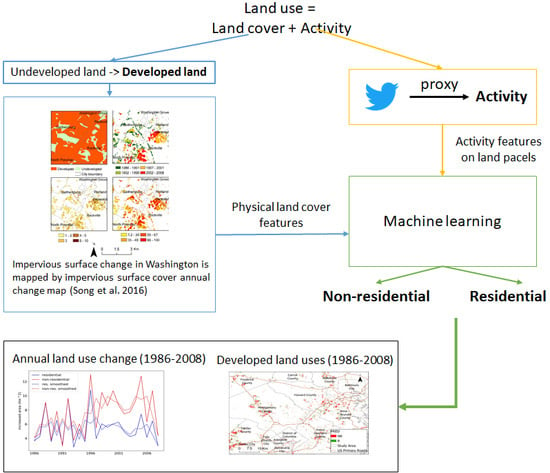
The primary objective of this research is to combine a remote-sensing-based land cover change product and georeferenced Tweets to identify the detailed land use of newly developed areas. We chose Washington D.C. as our study area. We associated Tweets with land parcels derived from the land cover map by the spatial relationship, and then modeled spatial-temporal patterns of how the parcels were used. We identified the newly-added residential and non-residential lands within the study area. Based on the results of the primary objective, our secondary objective was to estimate the geographic pattern of urban sprawl over the past three decades (i.e., the time span of satellite data) for residential and non-residential uses.

2. Study Area and Data

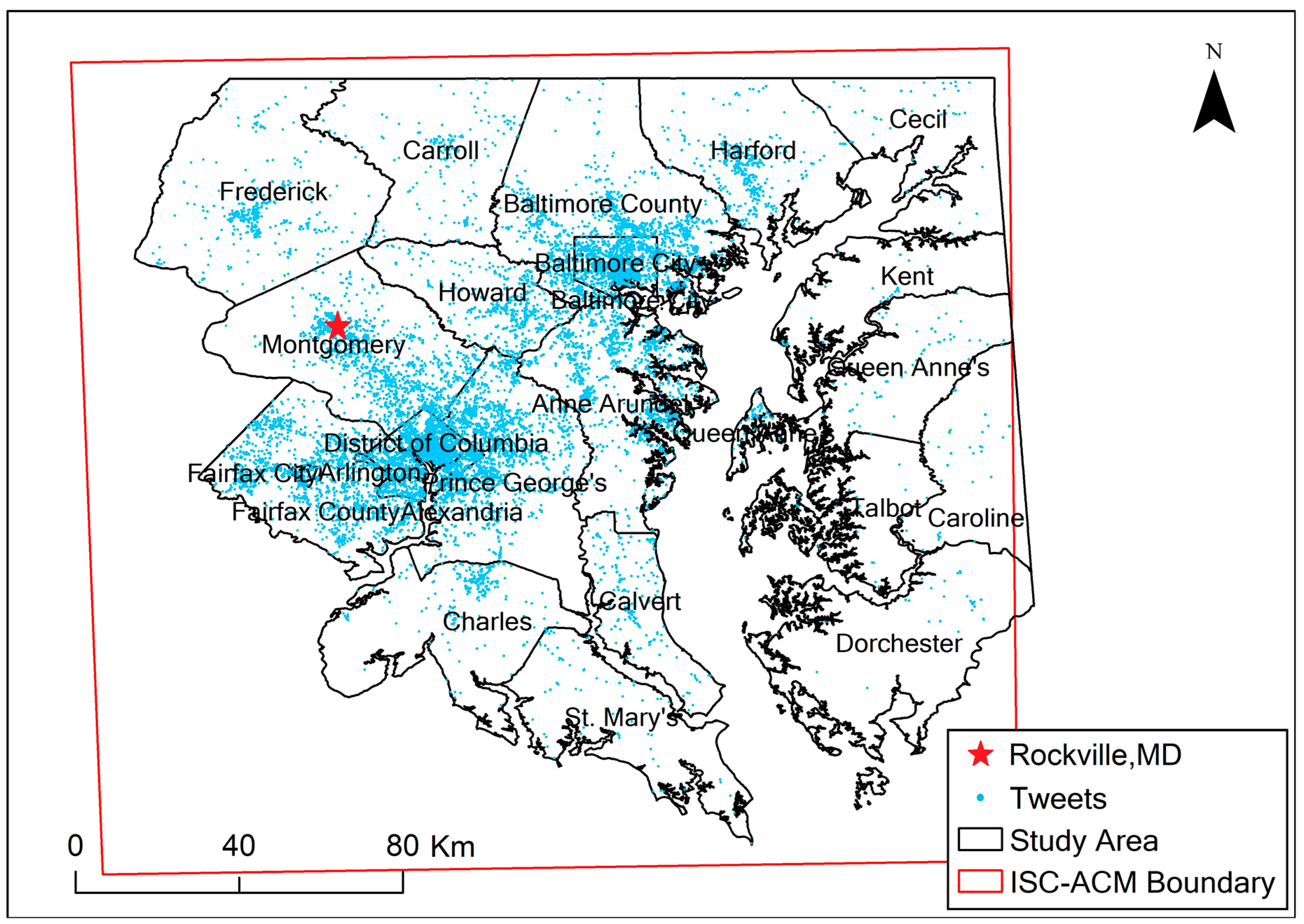
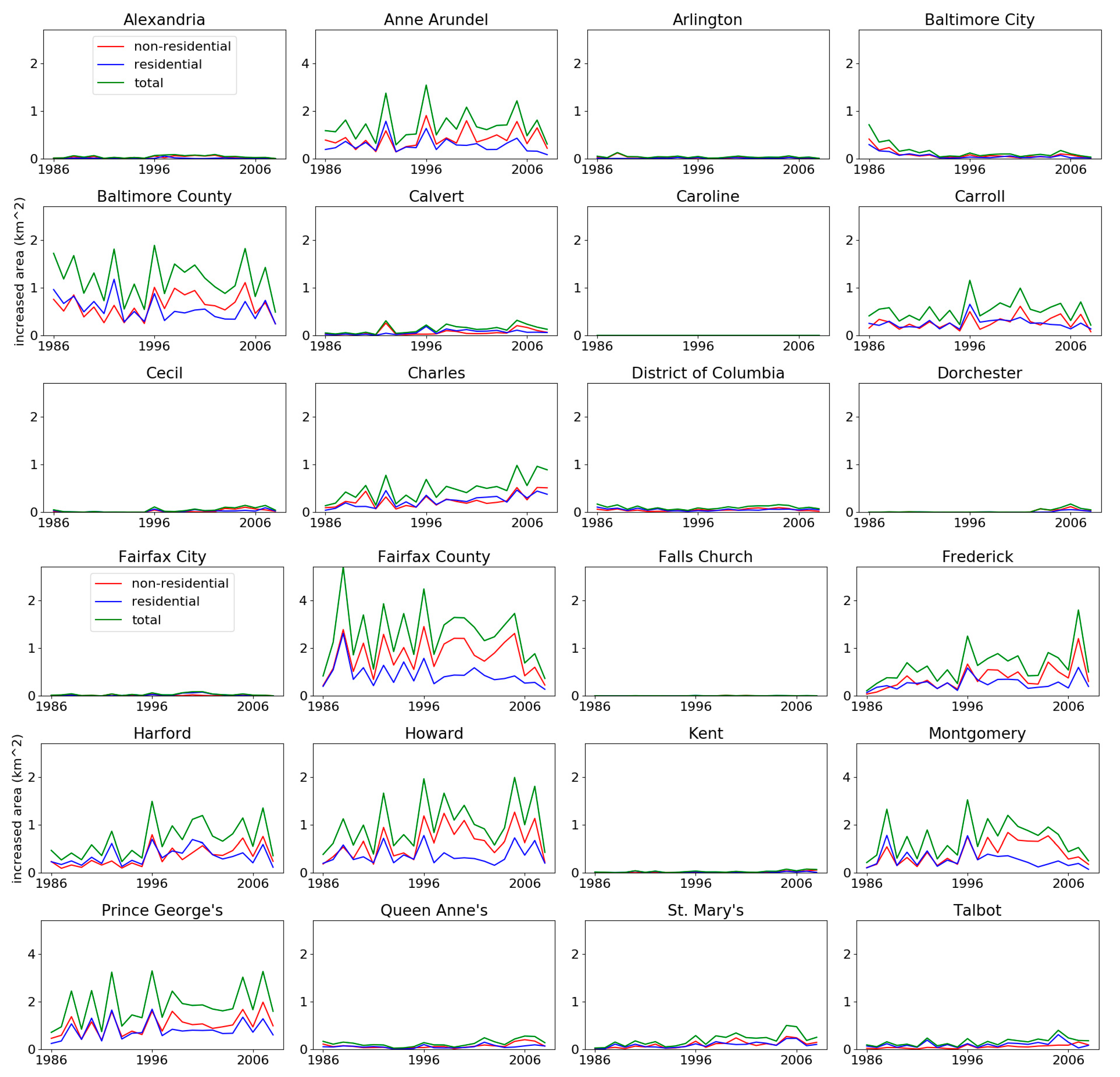
The Washington D.C.–Baltimore metropolitan area was selected as the study area, including the District of Columbia, four municipalities/counties in Virginia, and 17 counties in Maryland (Figure 1). The region is the capital of the United States and has experienced continued urban sprawl between 1984 and 2008 [10,26,27].
Five main data sources were used to model land use. The first source was a satellite-based Impervious Surface Cover Annual Change Map (ISC-ACM), generated at the University of Maryland [10]. The second data source was georeferenced Tweets from Twitter that are widely used for modeling human activities (e.g., References [28,29]). The third data source was zoning or land use maps collected from local urban planning departments for this region. The final two data sources were Google Maps and Google Street View, which were also used for the study region.
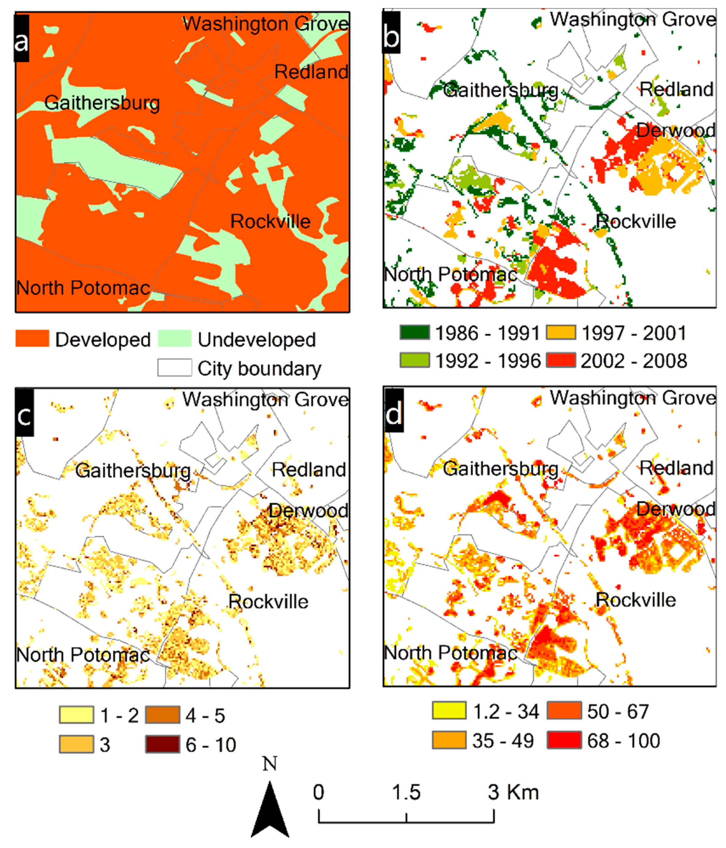
The Impervious Surface Cover Annual Change Map (ISC-ACM) is a suite of raster maps characterizing long-term urban land expansion at an annual frequency over the Washington DC–Baltimore metropolitan region. A complete description of this dataset is reported in References [10,27]. Here, we provide a concise summary of its key characteristics and the major steps of its development. The ISC-ACM consists of three map layers representing (1) the percentage increase of impervious surface cover per 30 × 30 m pixel for the period from 1986 to 2008; (2) the year during this period when the most significant impervious surface change occurred; and (3) the duration (unit: years) that a 30 m pixel was converted from undeveloped to developed (Figure 2b–d). These three change layers were simultaneously derived by applying an innovative change detection algorithm on a stack of annual percent impervious surface cover maps [10]. The stack of the annual impervious surface maps was in turn created using all available Landsat Thematic Mapper (TM) and Enhanced Thematic Mapper Plus (ETM+) imagery acquired during the 23 year period. Landsat images were converted in a series of processing steps to surface reflectance, seasonal composites, and annual percent impervious surface cover using regression tree and vector-based high-resolution training data obtained from the municipalities [27]. The overall accuracy of the change-year layer was 99.7%, as reported.
The second major data source used in this study, the georeferenced Tweets, were collected from October 2014 to April 2015 via the Twitter Public Streaming Application Program Interfaces (APIs). The final data set had about 11.12 million records. Given a small enough region, almost all georeferenced Tweets can be retrieved via the Twitter APIs [30]. There is no information about the position error of Tweets; however, as a reference, the median horizontal position error of a smartphone is reported to be between 5.0 and 8.5 m [20].
We also used available zoning maps or land use maps from planning departments that were the closest to 2008 as the reference for the actual land use. For counties in Maryland, this was the 2010 Maryland Land Use Land Cover Map [31]; for Washington D.C., it was the 2006 Land Use Map [32]; for counties in Virginia, we used 2015 zoning maps for each county [33,34,35,36]. The detailed land use types were re-categorized into two major land use classes: Undeveloped and developed. Undeveloped land use included forest, water, pasture, cropland, and other natural lands, while developed land use included two mutually exclusive sub-types: Residential and non-residential. Non-residential use included commercial, educational, hospital, industrial, etc. The official land use maps were used as a reference rather than the ground truth of land use as they were also not frequently updated, and therefore may not have reflected the actual land cover and land use after the time period we studied, as we discussed in Section 5.2 of this paper.
The final two data sources, Google Maps and Google Street View, were snapshots of land use ground truth in 2015 for the validation data sets and referred to land use in 2008.
It is noticeable that, for this study, the data products spanned different and non-overlapping time periods. The remote sensing data products were for 1986–2008, while the Tweets and Google data were for 2014 and 2015, respectively. Even though the Tweets were collected more recently than the physical signature data, any shifts to developed land (residential and non-residential), even those that occurred prior to 2008, were still expected to be in place since once land became developed, it was unlikely to revert back again to an undeveloped state. We discuss this issue of different data source timelines in more detail in Section 5.2.

3. Methodology

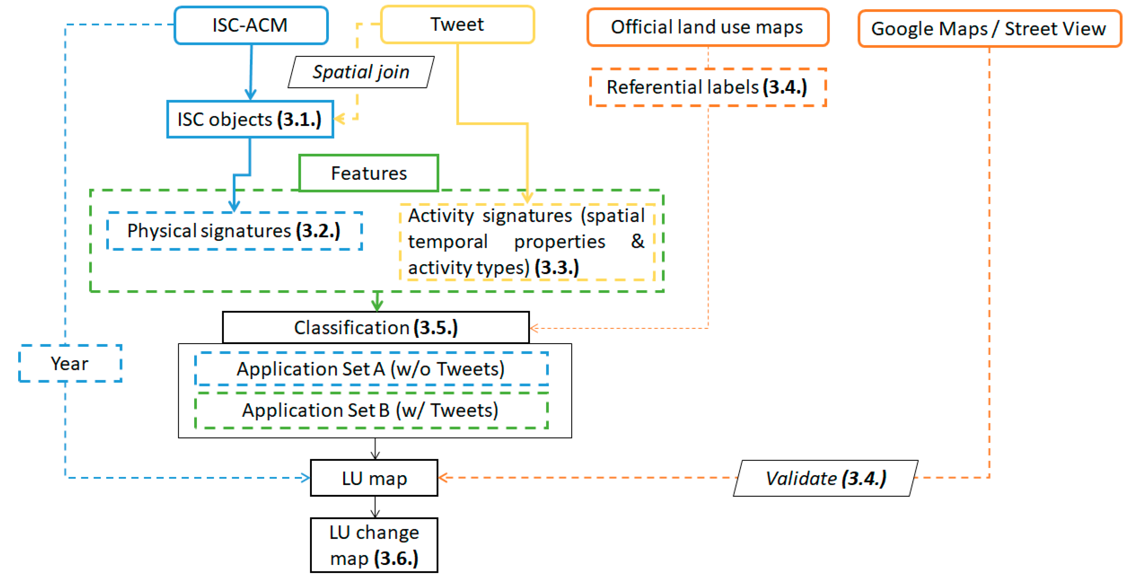
To identify land use change via our workflow (Figure 3), the change-detected pixels from the ISC-ACM were first grouped into parcels (denoted as ISC objects to differentiate them from parcels in the official land use maps) as the basic geographic units for aggregating and classifying physical vs. activity features. Georeferenced Tweets containing information about activities and their geolocations were spatially joined with all the ISC objects (Figure 3). Therefore, for each ISC object, a set of physical properties were derived from pixels in the ISC-ACM data as the physical signatures, and a set of activity properties were derived from associated Tweets as the activity signatures; together, these were combined to form the feature set of the ISC object. ISC objects were then associated with the official land use maps as a basis for categorizing if an ISC object would be included in the training set or not. Classification models were trained using the training set and were then applied to determine the land use type of the unlabeled ISC objects for 2008. Google Maps and Google Street View were used to validate the results. As the change year layer of the ISC-ACM (Figure 2b) showed the year land cover change for a pixel happened for 1986–2008, the classified results used this information to infer when land use changed and represented these changes in the land use change map (Figure 3). The following subsections discuss these steps in more detail.

3.1. Deriving Impervious Surface Cover Objects

Following an object-based image processing approach [37], connected component segmentation [38] was applied to adjacent group pixels in the ISC-ACM change-year layer classifying the pixels into objects. An object can be treated as a place or an area-of-interest (AOI, [39]), such as a plaza or a residential community occupying several pixels in the satellite images. It was also assumed that the construction of AOIs was continuous in time and space and thus adjacent pixels belonging to the same AOI should be labeled as the same year or adjacent years in the ISC-ACM change-year layer. Due to the ± 1 year uncertainty of the ISC-ACM [10], a two-year search radius was designed for the implementation of connected component segmentation using the image processing package Orfeo [40]. That is, if the change-year of two adjacent pixels was within ± 2 years, the two pixels were grouped into the same land parcel as an ISC object.

3.2. Building Physical Signatures for Impervious Surface Cover Objects

As an ISC object corresponds to a set of pixels in each ISC-ACM layer, five basic statistical metrics for pixel values of ISC objects in each layer were calculated as the physical signatures: minimum, maximum, mean, median, and standard deviation. In addition, the change magnitudes and change durations for each object were grouped by the change years, and the same five statistical metrics were calculated for these two properties for each year. Three morphological metrics of ISC objects were also included as part of the physical signature: perimeter, area, and the perimeter-area ratio [41].

3.3. Building Activity Signatures for Impervious Surface Cover Objects

Georeferenced Tweets were utilized as the proxy for human activities co-located with ISC objects. These activities provided another way to gain insights into different land uses. A key assumption that is discussed more fully in Section 5, and mentioned previously, was that although the Tweets were more recently collected than the physical signature data, any shifts to developed land that occurred even prior to 2008 were still expected to be in place. For preprocessing, Tweets from user accounts that potentially used location spoofing [42], and for this reason possibly falsified activity locations, were removed, excluding approximately 8% of the data set. The remaining Tweets were associated with the derived ISC objects by their location relationships.
Two types of activity patterns: Temporal patterns and topic patterns were derived by aggregating the Tweets for each ISC object. The time-varying number of Tweets in an average week has been frequently used as the activity signatures to characterize land use [14]. The temporal bin for aggregation was determined to be one hour. Tweets for an ISC object were aggregated by the day of the week first, regardless of the calendar date. Three metrics were then derived: hourly tweet volume, hourly user entropy, and hourly user volume to characterize temporal patterns.
The hourly tweet volume was defined as:
V o , d , h =   U T o , u , d , h
where o is the ID of an ISC object; u is the ID of a Twitter user; U is the set of user IDs; d is a day of the week; h ranges from 0 to 23 such that 0 represents the one-hour interval between 0:00–1:00 a.m.; T o , u , d , h represents the total number of Tweets from a unique user for an ISC object within the one-hour interval; and V o , d , h represents the hourly tweet volume. Residential places generally had lower volumes during week hours, while non-residential places had the opposite pattern.
It has been observed, however, that human behavior has a bursty nature, e.g., posting a large number of Tweets in a short time and then waiting for a period of time before tweeting again [43,44]. Therefore, a Shannon entropy measure [45] was employed to better profile the bursty phenomenon. Similar to the hourly tweet volume, hourly user entropy was thus defined as:
H o , d , h ( U ) = U p ( T o , u , d , h ) l o g b p ( T o , u , d , h )
where H o , d , h ( U ) is the Shannon entropy of users located at an ISC object o during the hourly interval h on the day of week d. p ( T o , u , d , h ) is the proportion of Tweets from a user among the total Tweets at the same ISC object during the same hourly interval on the same day of the week. It was expected that non-residential locations would have higher Shannon entropy values than residential locations since a greater number of people could stop by and leave their digital footprint online at non-residential places.
Hourly user volume counts user presence at a place within an hourly interval only once and thus represented both volume and diversity. It was defined as:
U o , u , d , h = { 1 ,     i f   T o , u , d , h > 0   0 ,     i f   T o , u , d , h = 0  
U V o , d , h =   U U o , u , d , h
where U V o , d , h is the hourly user volume and U o , u , d , h represents whether a user Tweets in an ISC object within a specific time interval. This index is not sensitive to the possible bursty pattern of tweeting activities and can differentiate situations involving no Tweets versus having all Tweets from one single user that cannot be characterized by the Shannon entropy.
Topic modeling derives a set of abstract hidden topics that occurs in a set of texts [46]. For deriving the topic pattern, Single Topic Latent Dirichlet Allocation (ST-LDA) [47] was utilized in this study as it is particularly designed to model topics in the Tweet text and has been used for analyzing human activities [29]. ST-LDA associates each Tweet with a single latent thematic topic that achieves the maximum probability to match the Tweet text. Each latent topic is represented as a weighted vector of vocabulary whose theme can be inferred by the word weights. We conceptualize that the latent thematic topics are also related to certain activities. For example, students may post Tweets with a topic whose top-weighted words are related to teachers, exams, and cohorts, which can be generalized as a “School Study” topic. The vector of topic counts for an ISC object formed the topic pattern for the object. We employed the same natural language processing (NLP) workflow integrating the ST-LDA model in a previous study of the Washington D.C. area [48].

3.4. Preparing Training, Validation and Undetermined Sets

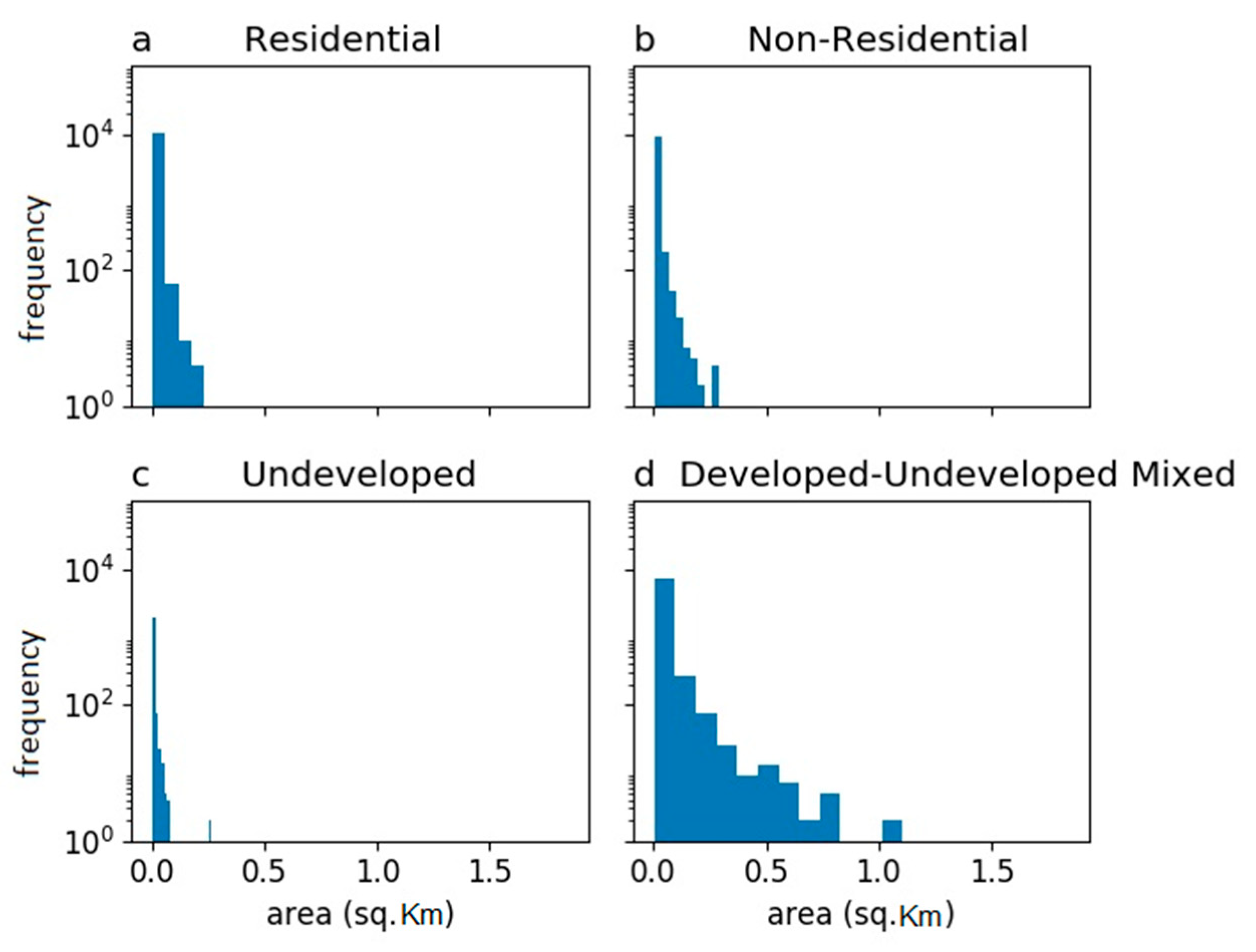
The categorized official land use maps were used to determine training and validation sets. If an ISC object was completely within a developed land use parcel, i.e., a residential or non-residential parcel, the object was assumed to be correctly labeled on the official land use map and was categorized as an entry of the Training Set for building the classification model in the next step. If an ISC object was partially or fully co-located with an undeveloped land parcel, or it was associated with two different types of developed land use, these objects were categorized as undetermined for predicting, by the classification model, as their land use type might have been mislabeled on the official land use maps. These undetermined ISC objects were further categorized into two sets: ISC objects with more than seven Tweets were categorized as Application Set A, the rest were categorized as an independent set denoted as Application Set B. As the smaller number of Tweets associated with objects in Application Set B did not allow for building a reliable activity signature, objects in this set were labeled by another classifier using the same training set, but only used the physical signature for classification. Among the unidentified ISC objects, 100 objects were randomly selected from both Application Set A and Application Set B, and these were denoted as Validation Set A and Validation Set B, respectively. The actual land use of the ISC objects as Validation Set A and B was visually checked using Google Maps and Google Street View to determine ground truth.

3.5. Training and Classification

We implemented the random forests algorithm [49] in scikit-learn [50] as the main classifier since this algorithm is robust for high-dimensional feature datasets and has better performance over other classifiers, as reported in Reference [51].
Ten-fold cross-validation [52] was used to evaluate the performance of the classification models building on the training dataset. Ten-fold cross-validation splits the training set into 10 equal-size folds and uses nine folds to build a classification model and one remaining fold to evaluate and then select the best model. Accuracy, Cohen’s Kappa coefficient [53], precision, recall, F1-score, and the area under the receiver operating characteristics curve (AUC) were used to undertake a comprehensive evaluation of the classifier. Precision is the percentage of true positive records in the dataset that are predicted as positive by the classifier. Recall is the percentage of records that are correctly predicted as positive in all positive records. The F1-score is the harmonic average of precision and recall [54]. AUC shows the probability that a classifier will rank a randomly chosen positive instance higher than a randomly chosen negative instance [55].
Two training processes were conducted on the same training set with different signature combinations: Both physical signatures and activity signatures (Appendix A for detailed attributes) were used for the first classification model to identify Application Set A; only physical signatures were used for the second classification model to identify Application Set B (no Tweets were associated with this set). In this analysis, each random forests model was composed of 256 trees [56]. The classification performances of the two models were evaluated by the 10-fold cross-validation. After the two application sets were classified, their corresponding testing sets were also applied to evaluate the two models, respectively, as the proxy for all objects.

3.6. Inferring Sprawl of Residential and Non-Residential Land Use in the Study Area

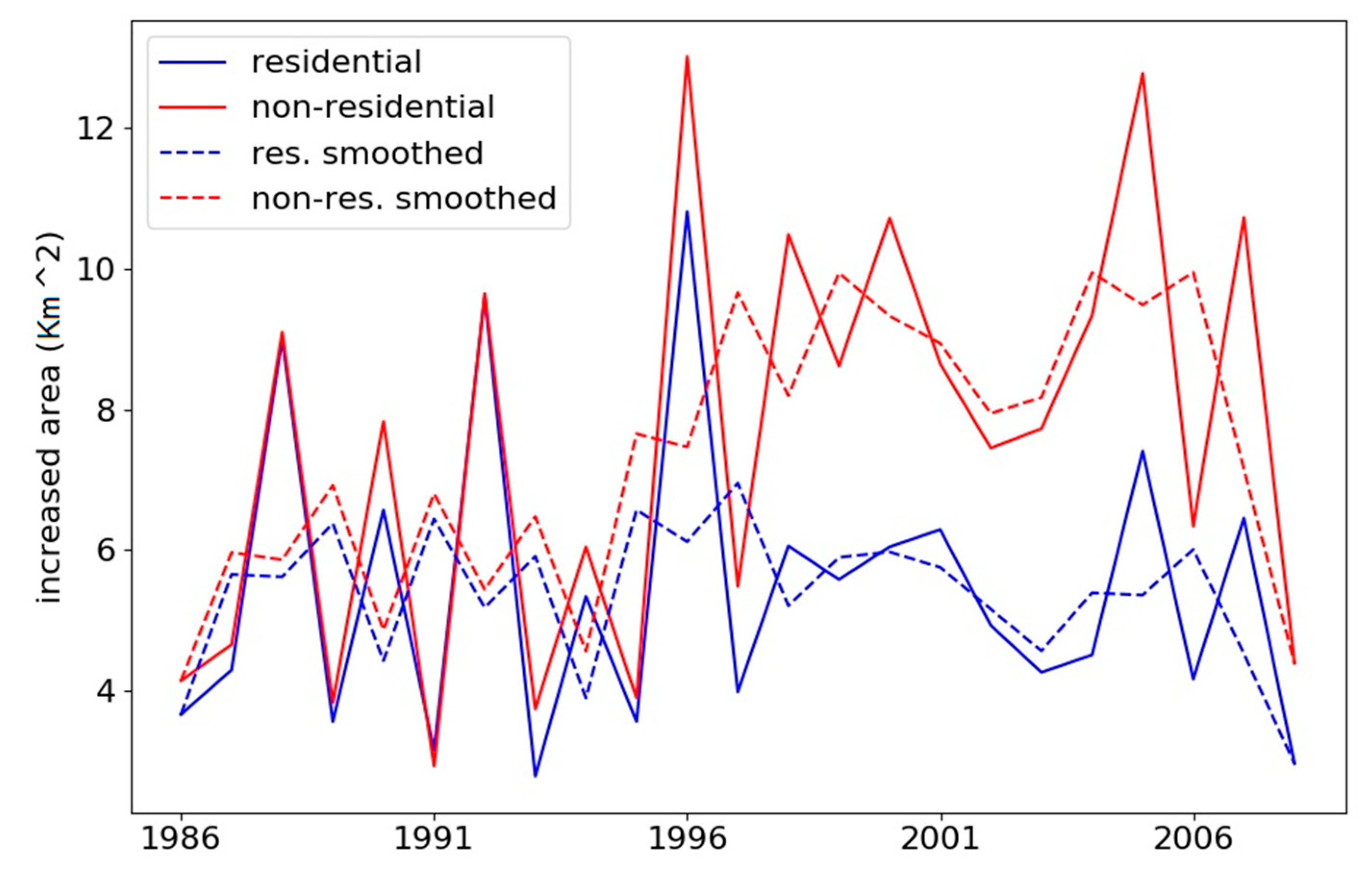
Once all unlabeled ISC objects in the two application sets were labeled by the classifier, the change from undeveloped land to developed land, including residential and non-residential uses in the period modeled by the ISC-ACM, was determined by counting the total area of pixels in a certain year labeled in the change-year layer of the map for each land use type.

4. Results

4.1. Identified Impervious Surface Cover Objects

There were 30,081 ISC objects in the study area: 20,182 developed (including 10,495 residential, and 9687 non-residential), 2087 as fully undeveloped, and 7812 as mixed, covering 300 km2 in total (Figure 4). For every type, the majority of ISC objects in the study area were small parcels less than 0.002 km2. 11,633 ISC objects had co-located Tweets, which accounted for 75.6% of the total area covered by all ISC objects.
The training set had 2520 ISC objects covering 24.2 km2 (including 1297 residential ISC objects covering 20.9 km2 and 1223 non-residential). Application Set A had 2174 ISC objects that were associated with more than seven Tweets and were thus qualified for labeling. The remaining ISC objects were included in Application Set B.

4.2. Activity Signatures of Impervious Surface Cover Objects

The NLP workflow using ST-LDA returned 100 topics that were derived from the full Tweet text set. Selected topic samples are visualized as word clouds in Appendix B.
By examining the spatial-temporal pattern and the semantic theme of the topics associated with the ISC objects, we found cases of ISC objects with mislabeled (i.e., outdated) land uses in the 2010 official land use map (Figure 5a,b). For example, four ISC objects corresponded to the South Germantown Recreational Park in Maryland, where three of the four objects were converted to different land uses between 2001 and 2002, and one object between 2005 and 2006. The activity signatures contributed to this finding as one of the ISC objects was associated with 50 Tweets by 31 users posted primarily between 11:00 and 22:00 (Figure 5c), for which at least 14 Tweets were associated with gaming as well as other recreation-related topics (Figure 5d). Following the same process, similar findings were applied to other ISC objects.

4.3. Comparison of Combining Physical and Activity Signatures to Individual Signatures

When both physical and activity signatures were used, the average accuracy for the 10-fold cross-validation of the classifier was 0.81, with a standard deviation of 0.03, and the best accuracy was 0.87. The average Kappa coefficient was 0.62, with a standard deviation of 0.06, which was in the range of substantial agreement [58]. The average AUC was also 0.81, with a standard deviation of 0.03. In addition, the precision and recall values were balanced (Table 1), meaning that the high accuracy was not achieved by consistently predicting all objects as one single type.
Using the two signatures separately achieved slightly poorer performance based on two additional 10-fold cross-validations on the classifiers with the same parameters (Table 2). The performance metrics based on using both signature combinations were all significantly higher than the results based on testing them independently using a t-test (p-value < 0.01).

4.4. Classification Model Performance on Validation Sets

In Validation Set A, there were 50 residential and 50 non-residential objects, while Validation Set B included 59 residential and 41 non-residential objects, based on visual inspection using Google Maps and Google Street View.
By evaluating the ISC objects in Validation Set A, predicted by the random forests model using the full training set and the same parameters for the best model in 10-fold cross-validation, as discussed in Section 4.3, the overall accuracy was 0.87, with a Kappa coefficient 0.74 and an AUC of 0.87 (Table 3). The three overall performance metrics were slightly better than most results in 10-fold cross-validation, while the validated accuracy was still in the range of two standard deviations of the mean 10-fold cross-validation accuracy. However, the model had a slightly lower performance for the precision of the non-residential type and for the recall of residential land use types than the results from the 10-fold cross-validation, even though the number of residential ISC objects was larger than the number of non-residential ISC objects in the training set.
The accuracy of an area’s estimation was subject to the areal extent of each object. Following the recommended practice for area-adjusted accuracy estimations in the remote sensing field [59], the estimated accuracy and estimated error matrix [60] were calculated in order to demonstrate the differences for the different land uses (Table 4).
For Validation Set B, the overall accuracy was 0.54, with a Kappa coefficient of 0.03 and an AUC of 0.51 (Table 5). The area-adjusted performance estimators were better than the object-based estimators (Table 6).

4.5. Modeling Pattern of Developed Land Use in the DC–Baltimore Metropolitan Are

The sprawl of built-up areas in the DC–Baltimore metropolitan area over time was mapped (Figure 6), based on combining the classification results of Section 4.4. Generally, newly developed (after 1986) non-residential places clustered along the main transportation corridors, e.g., the I-270 and Dulles Toll Road, while residential neighborhoods scattered around these non-residential places. In terms of the total area, the overall increase of residential areas was slightly smaller than for non-residential areas from 1986 to 2008 (Table 7). Using the estimated changed year in the change-year layer of the Impervious Surface Cover Annual Change Map (ISC-ACM), the temporal pattern of total land use sprawl was profiled (Figure 7). The overall time over which predicted developed land use sprawl occurred (both residential and non-residential) followed the same trend as that observed. The increase in non-residential areas was greater than residential areas after 1996.
The yearly increases of developed (residential and non-residential) areas in each administrative entity showed that sprawl mainly occurred in seven counties during the 1986–2008 period in Maryland, including Anne Arundel, Montgomery, and Prince George’s County, as well as in Fairfax County, Virginia (Figure 8). It was also observed that the increase in non-residential areas surpassed the increase in residential areas after 1996 for all counties but Fairfax County, where this increase started earlier in 1988.

5. Discussion

5.1. Contribution

In this study, we developed a framework that integrates socially-sensed human activities data and remotely sensed imagery as model inputs to identify detailed urban land use for the period 1986–2008. The output of the framework not only maps the spatial details of land use change but also profiles the trajectories of different land use types over time, which contributes to an understanding of the evolution of urban development as a complex system. The framework minimizes the dependence on traditional GIS data sets that may not be surveyed regularly and which are costly to undertake, such as land parcel footprint maps and street network maps. Since the original data sources, the Landsat imagery and georeferenced Tweets are both currently free to access, and the framework has the potential to be applied to other cities, especially those in developing countries, where cities are undergoing fast urbanization on a massive scale. For municipalities or counties in the US with zoning or land use maps, the output of this framework may help to address mapping errors in current maps.
This framework utilizes remote sensing imagery to model the physical signatures of land cover and georeferenced Tweets to model activity signatures associated with different land use types. The comparison of classification models shows the accuracy of the modeling using both signatures together is 0.04 and 0.06 higher than the model with the physical signature (i.e., remotely-sensed data) or the activity signature alone, respectively. After area adjustment, the former improvement increases to 0.10. The improvement is based on the distinguishable residential vs. non-residential landscape pattern found in the Washington D.C.–Baltimore region. This region has been experiencing suburbanization at a high rate where single-house communities with cul-de-sac designs are significantly different from commercial parcels in terms of morphology and the magnitude of impervious surfaces is increasing. This is not necessarily true for cities in other regions with more compact urban land parcel patterns, e.g., New York City, Beijing, and Manila. Activity signatures are expected to bring more value to these cases when differentiating the land use of parcels. In addition, different types of non-residential uses often have similarly high impervious surface cover that may be more difficult to distinguish using the physical signatures alone.
The higher values returned by the area-adjusted estimator compared to the object-based estimator in Section 4.4 was likely due to the large number of small objects in Application Set B and Validation Set B (objects with less than two pixels were 60% of the count, but accounted for 17% of the overall area in Validation Set B). Therefore, the area-adjusted accuracy of using a physical signature alone was a little better than the non-adjusted result, but still much lower than the result of the model utilizing both physical and activity signatures.
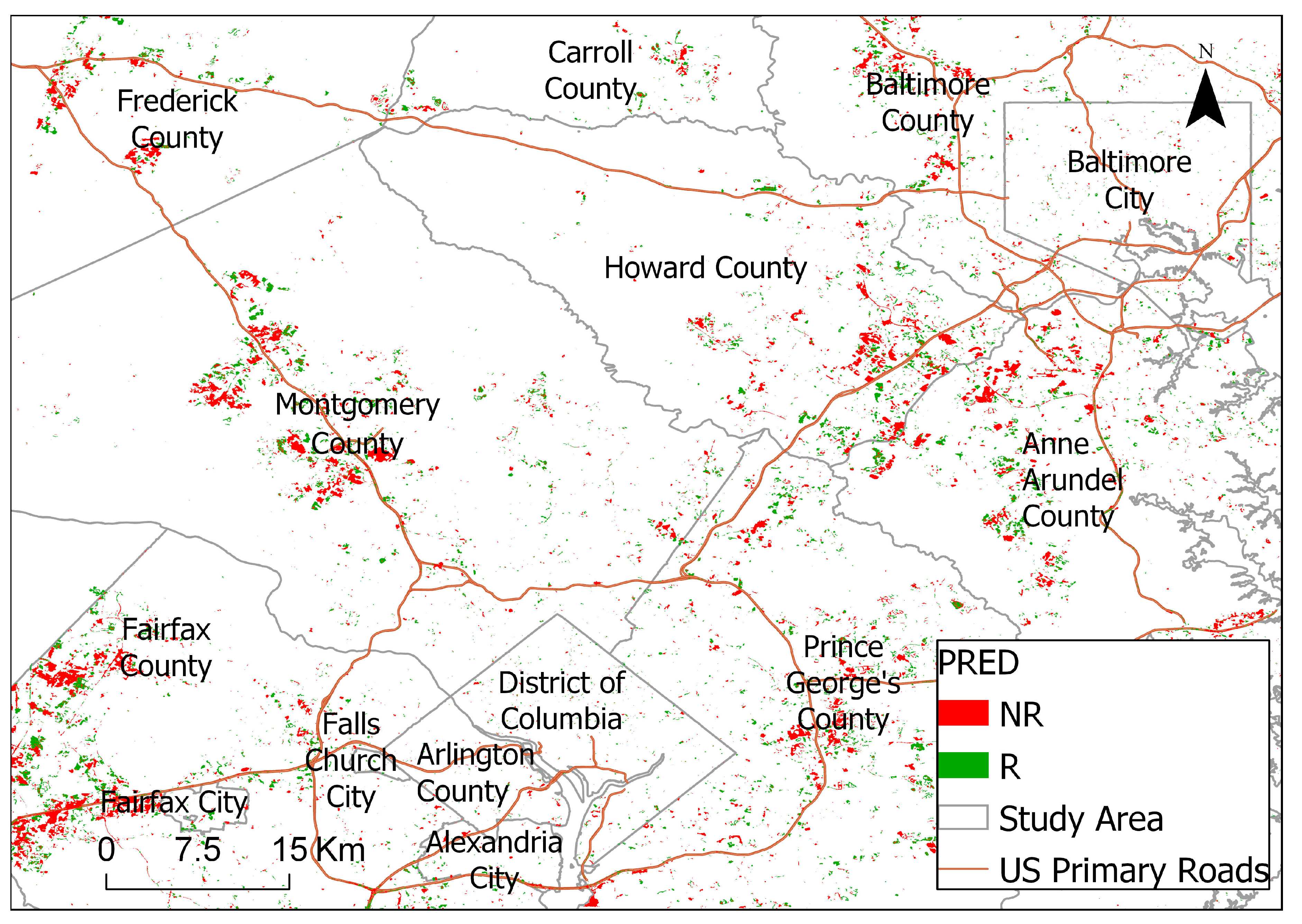
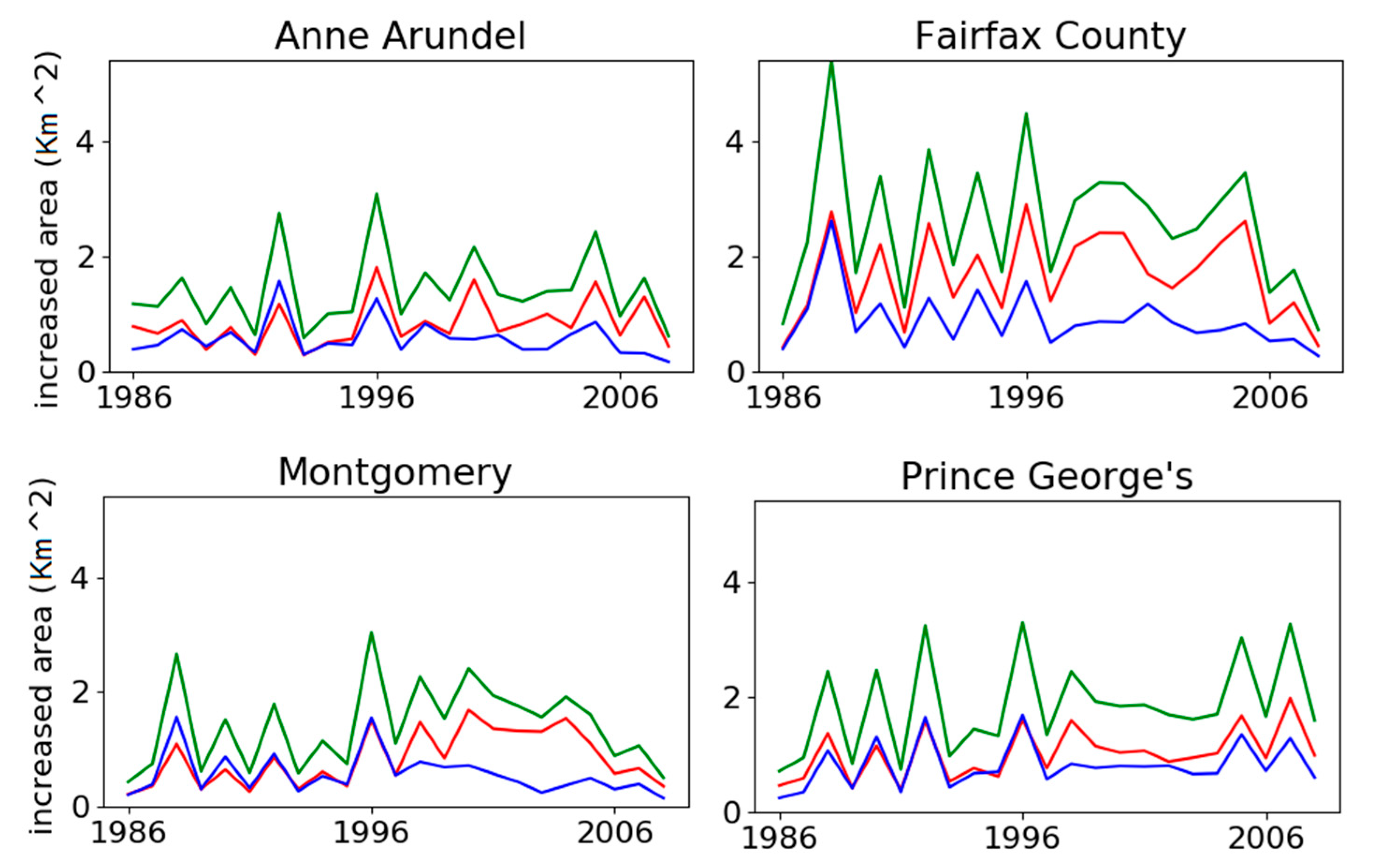
For modeling the sprawl of developed land, the higher the amount of non-residential over residential use in Section 4.5 for Montgomery County, MD, can be explained by the I-270 Technology Corridor stretching from the city of Bethesda to the city of Rockville, both within Montgomery County, MD. According to a local government report [61], this corridor is where over 18,000 business establishments have located, offering 72% of Montgomery County’s total employment, while 30% of the employees lived outside of the county, and most housing growth was estimated to be multi-family as of 2007. For Fairfax County, VA, the amount of increase could be explained by similar reasons, as there is the Dulles Technology Corridor connecting cities in Fairfax County and involve communities such as Tysons Corner, Reston, Herndon, Sterling, and Ashburn.

5.2. Source of Uncertainty

It should be acknowledged that temporal differences existed between the five different data sources employed in this study, which is a common issue for multi-source data fusion. Specifically, the most recent year of the remote sensing-based impervious surface map product was 2008, whereas Twitter data were collected for the year 2015. The seven-year gap between these two datasets may inevitably introduce some errors and differences, as land-use change between residential and non-residential on the newly developed land may occur. However, we believe that the temporal gap did not significantly alter the results of our study for the following reason. Potential errors could only be caused by the changes from residential to non-residential and vice versa on new urban land between 2008 and 2015. The amount of these specific types of land-use change was expected to be much less than general land-use conversions from undeveloped to developed between 1986 and 2008. Our independent validation using Google Maps and Google Street View supported this fact. We manually checked some ISC objects where Google Street View’s historical archive is available. The historical archive covers the period between 2007 and 2017, although the spatial coverage and the availability for certain years vary by location. We found no visual change for the ISC objects where the historical street views were available during the 2007–2017 period. Nevertheless, future research should focus on how more up-to-date remote sensing datasets could minimize the temporal difference between remote sensing and social sensing data and the impacts on reasoning with these data.
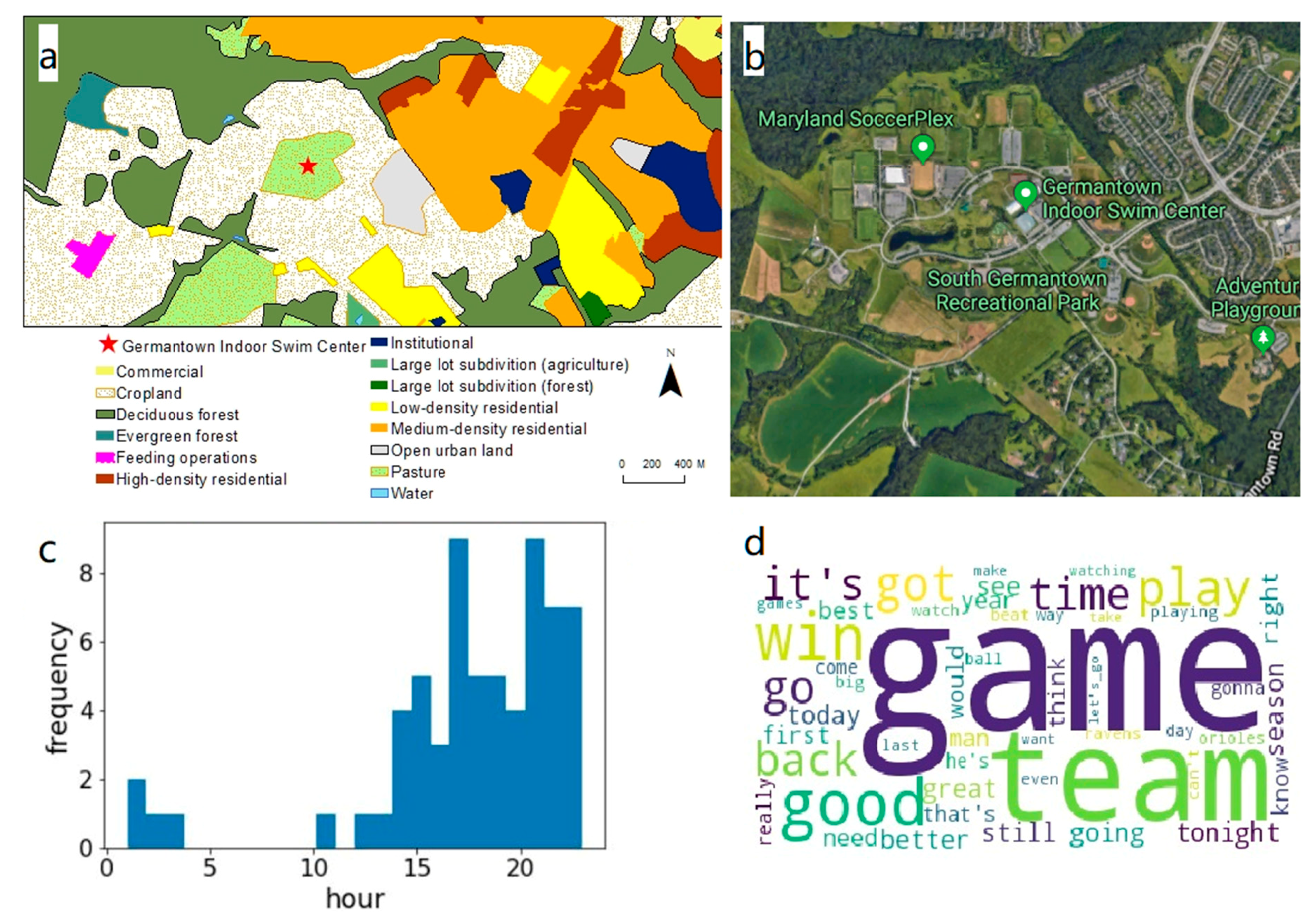
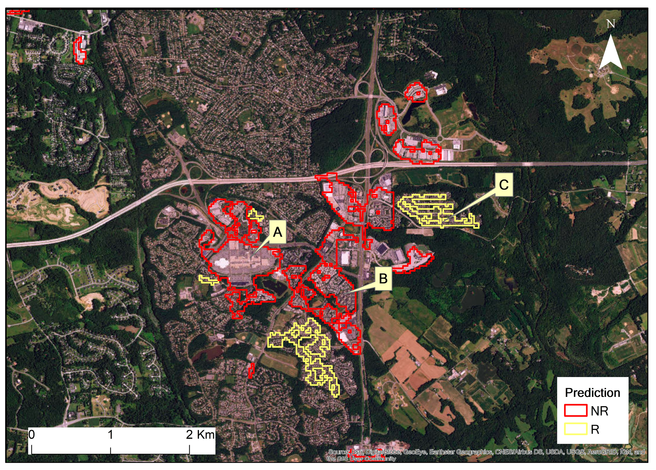
The tradeoff of this study was to define the spatial footprint of places from segmenting only remotely sensed imagery. Currently, image segmentation-based place footprints do not perfectly match the ground truth. As an example, using Application set A, parcel A, a commercial complex, and parcel C, a residential community with cul-de-sacs, were well identified (Figure 9). However, parcel B was based on a combination of commercial buildings in the North and some residential buildings in the South, and was labeled as non-residential. If a pixel in the commercial buildings part had been selected as a testing pixel, the label would be correct, but the attribution would be incorrect for other pixels. Unlike land cover objects, it is difficult to define the ground truth of a land use object, as a land use object may involve several land cover types. The boundary of a land use object may also be subjective, based on a person’s feelings about a place [62].
The topic features extracted as part of the activity signature analyses were observed to have high feature importance in random forests. This implies that topic features could be further investigated to classify more detailed non-residential land use types. Conceptually, each type of non-residential land use had unique corresponding activity types, for example, teaching or learning in schools and shopping in malls. If such activity information can be retrieved, it would be possible to use this information to identify more detailed non-residential land use types.
However, we should investigate a better model to associate the georeferenced Tweets with the land parcels to address the uncertainty from the positioning inaccuracy. In this study, we used the point-in-polygon spatial join to assign the Tweets to ISC objects, which may be sensitive to the positioning inaccuracy. In addition, due to the spatial bias of the georeferenced Tweets, as mentioned in the Introduction, further applications may still be limited to certain metropolitan areas that fit these demographics. The amount of available georeferenced Tweets in a study area may also influence the classification results.

6. Conclusions

We developed an innovative approach to identify land use types and change over time in a metropolitan area using both remotely sensed imagery and socially-sensed human activity data. We showed that adding twitter-based activity signatures to satellite-based physical signatures produced a higher accuracy (81%) for land use classification in this area than using physical signatures alone (72%). We produced a land use change map for the Washington D.C.–Baltimore metropolitan area during the 1986–2008 period and observed that 125.37 ± 10.56 km2 of new residential land use and 189.41 ± 10.56 km2 of new non-residential urban land use were developed. The temporal profile of annual urban sprawl showed that the increase of non-residential land use surpassed that of residential land use after 1996, with significant implications for urban planning. For future research, an investigation into how robust the proposed methods are with respect to Tweet positioning uncertainty could be undertaken using a sensitivity analysis. In addition, we will apply the proposed method to classify different types of non-residential land use and test its applicability in other metropolitan regions.

Author Contributions

Conceptualization, C.F. and X.-P.S.; methodology, C.F.; software, C.F.; validation, C.F.; formal analysis, C.F.; investigation, C.F.; resources, C.F.; data curation, C.F. and X.-P.S.; writing—original draft preparation, C.F.; writing—review and editing, C.F., X.-P.S., and K.S.; visualization, C.F.; supervision, K.S.

Funding

Cheng Fu is partially funded by European Union’s Horizon 2020 Research and Innovation Program, grant number 780754 and Xiao-Peng Song is partially funded by a NASA Earth and Space Fellowship, grant number NNX12AN92H.

Conflicts of Interest

The authors declare no conflict of interest.

Appendix A

Table A1. Feature groups and their index for the classifier model (ln stands for natural logarithm).
Signature TypeFeature GroupIndex
Activity signatureHourly tweet volume0~167
ln(Hourly tweet volume)168~335
Hourly user entropy336~503
ln(Hourly user entropy)504~671
Hourly user volume672~839
ln(Hourly user volume)840~1007
Physical signaturePerimeter, area, perimeter-area-ratio1008~1010
Activity signatureTopic counts1011~1110
Physical signatureStatistics of change year1111~1116
Statistics of change magnitude1116~1121
Statistics of change duration1121~1126
Statistics of change magnitude per year1126~1264
Statistics of change duration per year1265~1402

Appendix B

Figure A1. Selected topics from ST-LDA modeling. Topics are visualized as word-cloud. Larger font suggests more frequent. Suggested themes: (a) having dinner; (b) drinking; (c) fitness; (d) home entertainment.
Remotesensing 11 02965 g0a1

Appendix C

Figure A2. The increase in developed areas (non-residential and residential) by counties between 1986–2008.
Remotesensing 11 02965 g0a2

References

  1. United Nations World Urbanization Prospects: The 2014 Revision, Highlights (ST/ESA/SER.A/352); United Nations: New York, NY, USA, 2014.
  2. Seto, K.C.; Guneralp, B.; Hutyra, L.R. Global forecasts of urban expansion to 2030 and direct impacts on biodiversity and carbon pools. Proc. Natl. Acad. Sci. USA 2012, 109, 16083–16088. [Google Scholar] [CrossRef] [PubMed] [Green Version]
  3. Glaeser, E.L.; Kahn, M.E. The greenness of cities: Carbon dioxide emissions and urban development. J. Urban Econ. 2010, 67, 404–418. [Google Scholar] [CrossRef] [Green Version]
  4. Intergovernmental Panel on Climate Change Human Settlements, Infrastructure, and Spatial Planning. In Climate Change 2014 Mitigation of Climate Change; Cambridge University Press: Cambridge, UK, 2014; pp. 923–1000.
  5. Burby, R.J.; Deyle, R.E.; Godschalk, D.R.; Olshansky, R.B. Creating Hazard Resilient Communities through Land-Use Planning. Nat. Hazards Rev. 2000, 1, 99–106. [Google Scholar] [CrossRef] [Green Version]
  6. Iacono, M.; Levinson, D.; El-Geneidy, A. Models of Transportation and Land Use Change: A Guide to the Territory. J. Plan. Lit. 2008, 22, 323–340. [Google Scholar] [CrossRef]
  7. Waddell, P.; Wang, L.; Charlton, B.; Olsen, A. Microsimulating parcel-level land use and activity-based travel: Development of a prototype application in San Francisco. J. Transp. Land Use 2010, 3. [Google Scholar] [CrossRef]
  8. Batty, M.; Besussi, E.; Chin, N. Traffic, Urban Growth and Suburban Sprawl; Centre for Advanced Spatial Analysis: London, UK, 2003; Volume 44. [Google Scholar]
  9. Xian, G.; Homer, C.; Fry, J. Updating the 2001 National Land Cover Database land cover classification to 2006 by using Landsat imagery change detection methods. Remote Sens. Environ. 2009, 113, 1133–1147. [Google Scholar] [CrossRef] [Green Version]
  10. Song, X.P.; Sexton, J.O.; Huang, C.; Channan, S.; Townshend, J.R. Characterizing the magnitude, timing and duration of urban growth from time series of Landsat-based estimates of impervious cover. Remote Sens. Environ. 2016, 175, 1–13. [Google Scholar] [CrossRef]
  11. Herold, M.; Couclelis, H.; Clarke, K.C. The role of spatial metrics in the analysis and modeling of urban land use change. Comput. Environ. Urban Syst. 2005, 29, 369–399. [Google Scholar] [CrossRef]
  12. Liu, Y.; Liu, X.; Gao, S.; Gong, L.; Kang, C.; Zhi, Y.; Chi, G.; Shi, L. Social Sensing: A New Approach to Understanding Our Socioeconomic Environments. Ann. Assoc. Am. Geogr. 2015, 105, 512–530. [Google Scholar] [CrossRef]
  13. Pei, T.; Sobolevsky, S.; Ratti, C.; Shaw, S.; Li, T.; Zhou, C. A new insight into land use classification based on aggregated mobile phone data. Int. J. Geogr. Inf. Sci. 2014, 28, 1988–2007. [Google Scholar] [CrossRef] [Green Version]
  14. Frias-Martinez, V.; Soto, V.; Hohwald, H.; Frias-Martinez, E. Characterizing Urban Landscapes Using Geolocated Tweets. In Proceedings of the 2012 International Conference on Privacy, Security, Risk and Trust and 2012 International Confernece on Social Computing, Amsterdam, The Netherlands, 3–5 September 2012; IEEE: Piscataway, NJ, USA, 2012; pp. 239–248. [Google Scholar]
  15. Yuan, J.; Zheng, Y.; Xie, X. Discovering regions of different functions in a city using human mobility and POIs. In Proceedings of the 18th ACM SIGKDD International Conference on Knowledge Discovery and Data Mining—KDD ’12, Beijing, China, 12–16 August 2012; ACM Press: New York, NY, USA, 2012; p. 186. [Google Scholar]
  16. Nishi, K.; Tsubouchi, K.; Shimosaka, M. Extracting Land-Use Patterns using Location Data from Smartphones. In Proceedings of the the 1st International Conference on IoT in Urban Space, Rome, Italy, 27–28 October 2014; pp. 1–6. [Google Scholar]
  17. Zhou, X.; Zhang, L. Crowdsourcing functions of the living city from Twitter and Foursquare data. Cartogr. Geogr. Inf. Sci. 2016, 43, 393–404. [Google Scholar] [CrossRef]
  18. Li, X.; Zhang, C.; Li, W. Building block level urban land-use information retrieval based on Google Street View images. GISci. Remote Sens. 2017, 54, 819–835. [Google Scholar] [CrossRef]
  19. Kats, P.; Qian, C.; Kontokosta, C.; Sobolevsky, S. Twitter Activity Timeline as a Signature of Urban Neighborhood. arXiv 2017, arXiv:1707.06122. [Google Scholar]
  20. Zandbergen, P.A.; Barbeau, S.J. Positional Accuracy of Assisted GPS Data from High-Sensitivity GPS-enabled Mobile Phones. J. Navig. 2011, 64, 381–399. [Google Scholar] [CrossRef] [Green Version]
  21. Malik, M.M.; Lamba, H.; Nakos, C.; Pfeffer, J. Population Bias in Geotagged Tweets. In Proceedings of the 9th International Conference on Web and Social Media, Oxford, UK, 26–29 May 2015; pp. 18–27. [Google Scholar]
  22. Fonte, C.C.; Bastin, L.; See, L.; Foody, G.; Lupia, F. Usability of VGI for validation of land cover maps. Int. J. Geogr. Inf. Sci. 2015, 29, 1269–1291. [Google Scholar] [CrossRef] [Green Version]
  23. Rodriguez Lopez, J.M.; Heider, K.; Scheffran, J.; Miguel, J.; Lopez, R.; Heider, K.; Scheffran, J.; Alvarez-palacios, L. Frontiers of urbanization: Identifying and explaining urbanization hot spots in the south of Mexico City using human and remote sensing. Appl. Geogr. 2017, 79, 1–10. [Google Scholar] [CrossRef]
  24. Cervone, G.; Sava, E.; Huang, Q.; Schnebele, E.; Harrison, J.; Waters, N. Using Twitter for tasking remote-sensing data collection and damage assessment: 2013 Boulder flood case study. Int. J. Remote Sens. 2016, 37, 100–124. [Google Scholar] [CrossRef]
  25. Jia, Y.; Ge, Y.; Ling, F.; Guo, X.; Wang, J.; Wang, L.; Chen, Y.; Li, X. Urban Land Use Mapping by Combining Remote Sensing Imagery and Mobile Phone Positioning Data. Remote Sens. 2018, 10, 446. [Google Scholar] [CrossRef] [Green Version]
  26. Goetz, S.J.; Smith, A.J.; Jantz, C.; Wright, R.K.; Prince, S.D.; Mazzacato, M.E.; Melchior, B. Monitoring and predicting urban land use change applications of multi-resolution multi-temporal satellite data. In Proceedings of the IGARSS 2003, 2003 IEEE International Geoscience and Remote Sensing Symposium, Proceedings (IEEE Cat. No.03CH37477), Toulouse, France, 21–25 July 2003; IEEE: Piscataway, NJ, USA, 2003; Volume 3, pp. 1567–1569. [Google Scholar]
  27. Sexton, J.O.; Song, X.-P.; Huang, C.; Channan, S.; Baker, M.E.; Townshend, J.R. Urban growth of the Washington, D.C.–Baltimore, MD metropolitan region from 1984 to 2010 by annual, Landsat-based estimates of impervious cover. Remote Sens. Environ. 2013, 129, 42–53. [Google Scholar] [CrossRef]
  28. Jenkins, A.; Croitoru, A.; Crooks, A.T.; Stefanidis, A. Crowdsourcing a collective sense of place. PLoS ONE 2016, 11, e0152932. [Google Scholar] [CrossRef] [Green Version]
  29. Hong, L.; Fu, C.; Torrens, P.; Frias-Martinez, V. Understanding Citizens’ and Local Governments’ Digital Communications During Natural Disasters. In Proceedings of the 2017 ACM on Web Science Conference—WebSci ’17, Troy, NY, USA, 25–28 June 2017; ACM Press: New York, NY, USA, 2017; pp. 141–150. [Google Scholar]
  30. Morstatter, F.; Pfeffer, J.; Liu, H.; Carley, K.M. Is the Sample Good Enough? Comparing Data from Twitter’s Streaming API with Twitter’s Firehose. In Proceedings of the International AAAI Conference on Weblogs and Social Media (ICWSM), Boston, MA, USA, 8–11 July 2013; pp. 400–408. [Google Scholar]
  31. Maryland Department of Planning 2010 Maryland Land Use Land Cover Map. Available online: http://mdpgis.mdp.state.md.us/landuse/imap/index.html (accessed on 20 June 2010).
  32. DC Office of Planning Existing Land Use Maps. Available online: https://planning.dc.gov/page/existing-land-use-maps (accessed on 1 October 2016).
  33. Arlington County Zoning Map, Arlington County, VA. Available online: http://gis.arlingtonva.us/gallery/map.html?webmap=1e4706ab574a462a8dcc6a6c182b0004 (accessed on 20 June 2010).
  34. City of Alexandria City of Alexandria 2015 Zoning Map. Available online: https://www.alexandriava.gov/uploadedFiles/gis/info/Zoning2015.pdf (accessed on 20 June 2010).
  35. City of Falls Church Official Zoning District Map. Available online: http://www.fallschurchva.gov/DocumentCenter/View/690 (accessed on 20 June 2010).
  36. Fairfax County GIS & Mapping Service Branch Zoning, Fairfax County, VA. Available online: http://data-fairfaxcountygis.opendata.arcgis.com/datasets/zoning (accessed on 1 October 2016).
  37. Hussain, M.; Chen, D.; Cheng, A.; Wei, H.; Stanley, D. Change detection from remotely sensed images: From pixel-based to object-based approaches. ISPRS J. Photogramm. Remote Sens. 2013, 80, 91–106. [Google Scholar] [CrossRef]
  38. Haralick, R.; Shapiro, L. Image segmentation techniques. CVGIP Image Underst. 1985, 29, 100–132. [Google Scholar]
  39. Hu, Y.; Gao, S.; Janowicz, K.; Yu, B.; Li, W.; Prasad, S. Extracting and understanding urban areas of interest using geotagged photos. Comput. Environ. Urban Syst. 2015, 54, 240–254. [Google Scholar] [CrossRef]
  40. Inglada, J.; Christophe, E. The Orfeo Toolbox remote sensing image processing software. In Proceedings of the 2009 IEEE International Geoscience and Remote Sensing Symposium, Cape Town, South Africa, 12–17 July 2009; pp. 733–736. [Google Scholar]
  41. Herold, M.; Scepan, J.; Clarke, K.C. The use of remote sensing and landscape metrics to describe structures and changes in urban land uses. Environ. Plan. A 2002, 34, 1443–1458. [Google Scholar] [CrossRef] [Green Version]
  42. Zhao, B.; Sui, D.Z. True lies in geospatial big data: Detecting location spoofing in social media. Ann. GIS 2017, 23, 1–14. [Google Scholar] [CrossRef]
  43. Vázquez, A.; Oliveira, J.; Dezsö, Z.; Goh, K.; Kondor, I.; Barabási, A. Modeling bursts and heavy tails in human dynamics. Phys. Rev. E 2006, 73, 036127. [Google Scholar] [CrossRef] [PubMed] [Green Version]
  44. Barabasi, A.-L. The origin of bursts and heavy tails in human dynamics. Nature 2005, 435, 207–211. [Google Scholar] [CrossRef] [Green Version]
  45. Zhong, C.; Arisona, S.M.M.; Huang, X.; Batty, M.; Schmitt, G. Detecting the dynamics of urban structure through spatial network analysis. Int. J. Geogr. Inf. Sci. 2014, 28, 2178–2199. [Google Scholar] [CrossRef]
  46. Blei, D. Probabilistic topic models. In Proceedings of the 17th ACM SIGKDD International Conference Tutorials—KDD ’11 Tutorials, San Diego, CA, USA, 21–24 August 2011. [Google Scholar]
  47. Hong, L.; Yang, W.; Resnik, P.; Frias-Martinez, V. Uncovering Topic Dynamics of Social Media and News: The Case of Ferguson. In Proceedings of the International Conference on Social Informatics, Bellevue, WA, USA, 11–14 November 2016; Volume 10046 LNCS, pp. 240–256. [Google Scholar]
  48. Fu, C.; McKenzie, G.; Frias-Martinez, V.; Stewart, K. Identifying spatiotemporal urban activities through linguistic signatures. Comput. Environ. Urban Syst. 2018, 72, 25–37. [Google Scholar] [CrossRef]
  49. Segal, M.R. Machine Learning Benchmarks and Random Forest Regression; Division of Biostatistics, University of California: San Francisco, CA, USA, 2004; pp. 1–14. [Google Scholar]
  50. Pedregosa, F.; Varoquaux, G.; Gramfort, A.; Michel, V.; Thirion, B.; Grisel, O.; Blondel, M.; Prettenhofer, P.; Weiss, R.; Dubourg, V.; et al. Scikit-learn: Machine Learning in Python. J. Mach. Learn. Res. 2011, 12, 2825–2830. [Google Scholar]
  51. Caruana, R.; Niculescu-Mizil, A. An empirical comparison of supervised learning algorithms. In Proceedings of the 23rd International Conference on Machine Learning, Pittsburgh, PA, USA, 25–29 June 2006; pp. 161–168. [Google Scholar]
  52. Kohavi, R. A Study of Cross-Validation and Bootstrap for Accuracy Estimation and Model Selection. Int. Jt. Conf. Artif. Intell. 1995, 14, 1137–1143. [Google Scholar]
  53. Cohen, J. A coefficient of agreement for nominal scales. Educ. Psychol. Meas. 1960, 20, 37–46. [Google Scholar] [CrossRef]
  54. Han, J.; Kamber, M.; Pei, J. Data Mining: Concepts and Techniques, 3rd ed.; Morgan Kaufmann Publishers: Waltham, MA, USA, 2012. [Google Scholar]
  55. Fawcett, T. An introduction to ROC analysis. Pattern Recognit. Lett. 2006, 27, 861–874. [Google Scholar] [CrossRef]
  56. Oshiro, T.M.; Perez, P.S.; Baranauskas, J.A. How Many Trees in a Random Forest? Mach. Learn. Data Mining Pattern Recognit. 2012, 7376, 154–168. [Google Scholar]
  57. Montgomeryparks.org MEDIA ADVISORY: Maryland’s First Miracle League Field Possibly Coming to South Germantown Recreational Park. Available online: https://www.montgomeryparks.org/media-advisory-marylands-first-miracle-league-field-possibly-coming-to-south-germantown-recreational/ (accessed on 7 February 2018).
  58. Landis, J.R.; Koch, G.G. The Measurement of Observer Agreement for Categorical Data. Biometrics 1977, 33, 159–174. [Google Scholar] [CrossRef] [Green Version]
  59. Olofsson, P.; Foody, G.M.; Herold, M.; Stehman, S.V.; Woodcock, C.E.; Wulder, M.A. Good practices for estimating area and assessing accuracy of land change. Remote Sens. Environ. 2014, 148, 42–57. [Google Scholar] [CrossRef]
  60. Olofsson, P.; Foody, G.M.; Stehman, S.V.; Woodcock, C.E. Making better use of accuracy data in land change studies: Estimating accuracy and area and quantifying uncertainty using stratified estimation. Remote Sens. Environ. 2013, 129, 122–131. [Google Scholar] [CrossRef]
  61. Tate, L.M.; Suarez, S.; Akundi, K.; Pamela, Z.; Koempel, W. The MD-355/I-270 Technology Corridor Montgomery County, Maryland; Research & Technology Center, Montgomery County Planning Department: Silver Spring, MD, USA, 2007. [Google Scholar]
  62. Tuan, Y.F. Space and Place: Humanistic Perspective. In Philosophy in Geography; Gale, S., Olsson, G., Eds.; Springer: Dordrecht, The Netherlands, 1979; pp. 387–427. [Google Scholar]
Figure 1. Geography of the study area. ISC-ACM stands for the Impervious Surface Cover Annual Change Map. Tweets were collected from October 2014 to April 2015.
Remotesensing 11 02965 g001
Figure 2. The area North of the city of Rockville, MD (marked as a star in Figure 1) on the official land use map and the Impervious Surface Cover Annual Change Map (ISC-ACM) set layers: (a) Land use recategorized from the 2010 Maryland Land Use Land Cover Map, (b) change year layer (period of most significant impervious surface increase), (c) change duration layer (duration of impervious surface increase in terms of the number of years), and (d) change magnitude layer (percentage of impervious surface increase).
Remotesensing 11 02965 g002
Figure 3. Workflow for combining physical and activity signatures to identify urban land use types. Colors indicate different data sources involved: Blue is the remotely sensed data only; yellow is the Twitter data only; and green involves both remotely sensed data and Twitter data. Orange involves data for referencing the land uses. Solid arrow lines indicate the main data processing and modeling flow. Dashed arrow lines indicate the inferring process.
Remotesensing 11 02965 g003
Figure 4. Frequency distribution of ISC objects by land use type. The X-axis represents the size of ISC objects and the Y-axis represents the amount of ISC objects.
Remotesensing 11 02965 g004
Figure 5. The South Germantown Recreational Park on the 2010 Maryland Land Use Land Cover Map (a) and on Google Maps (2018) (b). The land parcels in which the park is located (marked as the red star on the official land use map as a reference) are mislabeled as pasture and cropland, although the sports facilities were reported to be in use in 2009 [57]. Time frequency of Tweets (c) and the top topic associated with an ISC object at the location of the South Germantown Recreational Park visualized as a word cloud (d).
Remotesensing 11 02965 g005
Figure 6. Non-residential and residential areas developed between 1986 and 2008 in the Washington D.C.–Baltimore region by the three sub data sets. The values of the training set are used as ground truths from land use maps. The values of the other two labeling sets are based on modeling predictions.
Remotesensing 11 02965 g006
Figure 7. Residential and non-residential area increases in the study area by year using the same approach as Figure 6. The smoothed curves are based on three-year moving window averages.
Remotesensing 11 02965 g007
Figure 8. The annual increases in the developed areas (non-residential and residential) of the four selected counties from 1986 to 2008. The annual increases of all counties in the study area are in Appendix C.
Remotesensing 11 02965 g008
Figure 9. Detailed ISC object classification result of Application Set A near Bowie, MD. R: residential. NR: non-residential.
Remotesensing 11 02965 g009
Table 1. Detailed classification report of selected cross-validation on features from both physical and activity signatures (accuracy: 0.87, Kappa coefficient: 0.74, AUC: 0.87).
PrecisionRecallF1-Score
Non-residential0.890.840.86
Residential0.850.900.88
Average0.870.870.87
Table 2. Model performance of 10-fold cross-validation on three signature combinations.
Signature CombinationAverage AccuracyAverage KappaAverage AUC
Physical + activity0.810.620.81
Physical only0.770.540.77
Activity only0.750.490.75
Table 3. Detailed classification report on Validation Set A based on the 100 validation ISC objects (accuracy: 0.87, Kappa coefficient: 0.74, AUC: 0.87).
PrecisionRecallF1-Score
Non-residential0.810.960.88
Residential0.950.780.86
Average0.880.870.87
Table 4. Area-adjusted accuracy and error matrix on the 100 validation ISC objects in Validation Set A. The margin of error is based on 1.96 times the standard error of the estimators, which provides a 95% confidence.
Estimated Overall Accuracy0.81 ± 0.01
Estimated PrecisionEstimated Recall
Non-residential0.75 ± 0.010.98 ± 0.003
Residential0.96 ± 0.010.61 ± 0.006
Table 5. Detailed classification report on the Validation Set B based on the 100 validation ISC objects (Accuracy: 0.54, Kappa coefficient: 0.02, AUC: 0.51).
PrecisionRecallF1-Score
Non-residential0.640.620.63
Residential0.380.410.39
Avg.0.550.540.54
Table 6. Area-adjusted accuracy and error matrix on the 100 validation ISC objects in Validation Set B. The margin of error was based on 1.96 times the standard error of the estimators, which provided a 95% confidence.
Estimated Overall Accuracy0.72 ± 0.04
Estimated PrecisionEstimated Recall
Non-residential0.80 ± 0.040.78 ± 0.001
Residential0.55 ± 0.090.58 ± 0.03
Table 7. Areas of residential and non-residential land use using the same approach as Figure 6. The unit of values is km2. The margin of error is based on 1.96 times the standard error of the estimators, which provides a 95% confidence.
ResidentialNon-ResidentialTotal
Training: Truth20.6324.1444.77
Application Set A: Predicted40.58 ± 1.1991.07 ± 1.19131.65
Application Set B: Predicted64.16 ± 9.3774.20 ± 9.37138.36
Total125.37 ± 10.56189.41 ± 10.56314.78

