An Efficient Imaging Algorithm for GNSS-R Bi-Static SAR


Abstract
1. Introduction
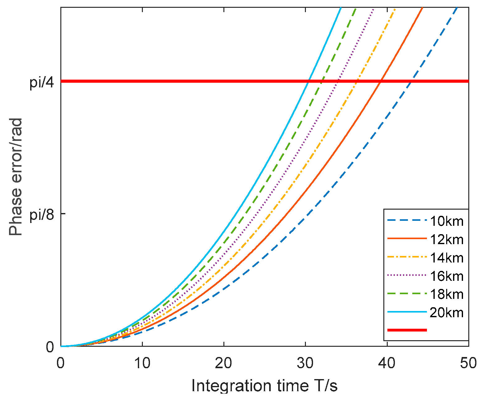
- The complex expression for range history: The range history is due to the motion of both the GNSS satellite and the receiving platform, which makes it extremely difficult to obtain a precise analytical solution to the stationary phase point of the Doppler phase.
- The translational variant Doppler history: Unlike mono-static SAR, the Doppler history of the echo signal of GNSS-R BSAR is translationally variant since the trajectories of the transmitter and the receiver are non-parallel and their velocities are also different. This means that imaging becomes a two-dimensional spatially varying filtering process.
2. Materials and Methods
2.1. Modelling and Analysis
- The spatially varying Doppler centroid: It is formed by the linear component of the residual transmitter range and represented by the spatially varying delay time tdk. This means the equivalent squint angle is also spatially varying.
- The translational variant Doppler FM rate: It is formed by the constant component of the residual transmitter range and represented by the shifting factor Rshiftk. The shifting factor Rshiftk indicates that the echo data for targets with the same minimum receiver range (thus the same Doppler FM rate) will not appear in the same range cell. In other words, the signals that appear in the same range cell have a different Doppler FM rate.
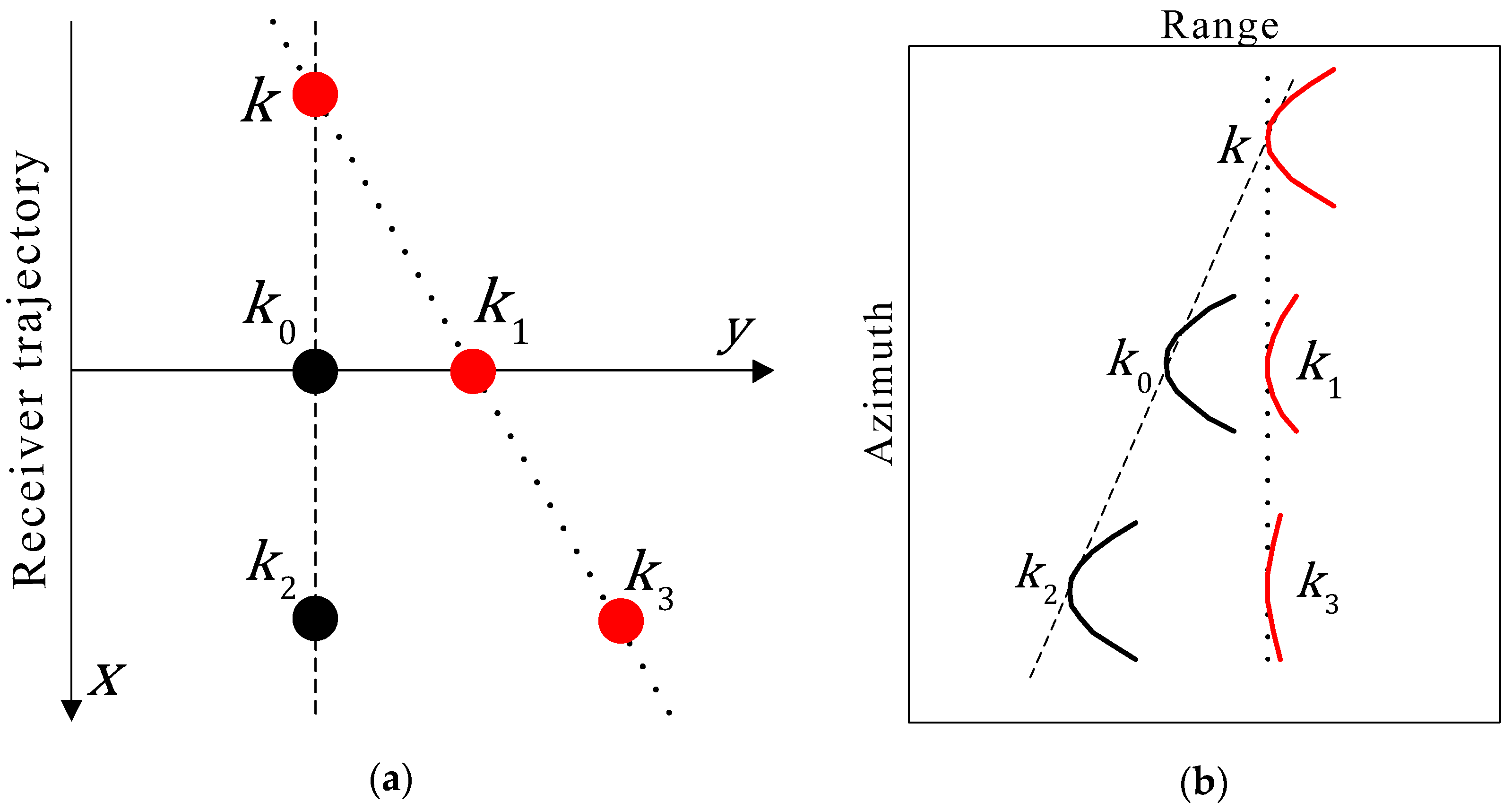
- The scene space in which the echo data are received.
- The echo space in which the echo data are stored and processed.
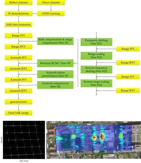
2.2. Imaging Methods
2.2.1. Bulk Compensation and Range Compression
2.2.2. Residual RCMC
- The scaling operation is not applied to the range frequency axis, but to the range time axis, and thus in some sense, it is more appropriate to name the modified algorithm the range scaling algorithm rather than the frequency scaling algorithm.
- The scaling of the range time needs four multiplications rather than three as in the frequency scaling algorithm.
- The scaling factors should all be adapted to the new application.
2.2.3. Azimuth Phase Perturbation
- The constant component πat03: It changes the phase of the signal according to the position of the target, which can be ignored when only the amplitude of the image is concerned. Here:
- The first order component 3πat02(t − t0): It adds a small spatially varying Doppler shift to the signal. This shift is a quadratic function of the azimuth time t, which can be incorporated into the Doppler shift caused by the residual transmitter range, i.e.,
- The second order compound 3πat0(t − t0) 2: It equalizes the Doppler FM rate along the range cell.
- The third order compound πa(t − t0)3: It is a cubic phase modulation, which is the same for all targets. It is far smaller than the phase modulation caused by the receiver motion, which can be ignored during the derivation of the azimuth stationary phase point of the signal.
2.2.4. Azimuth Compensation
3. Results
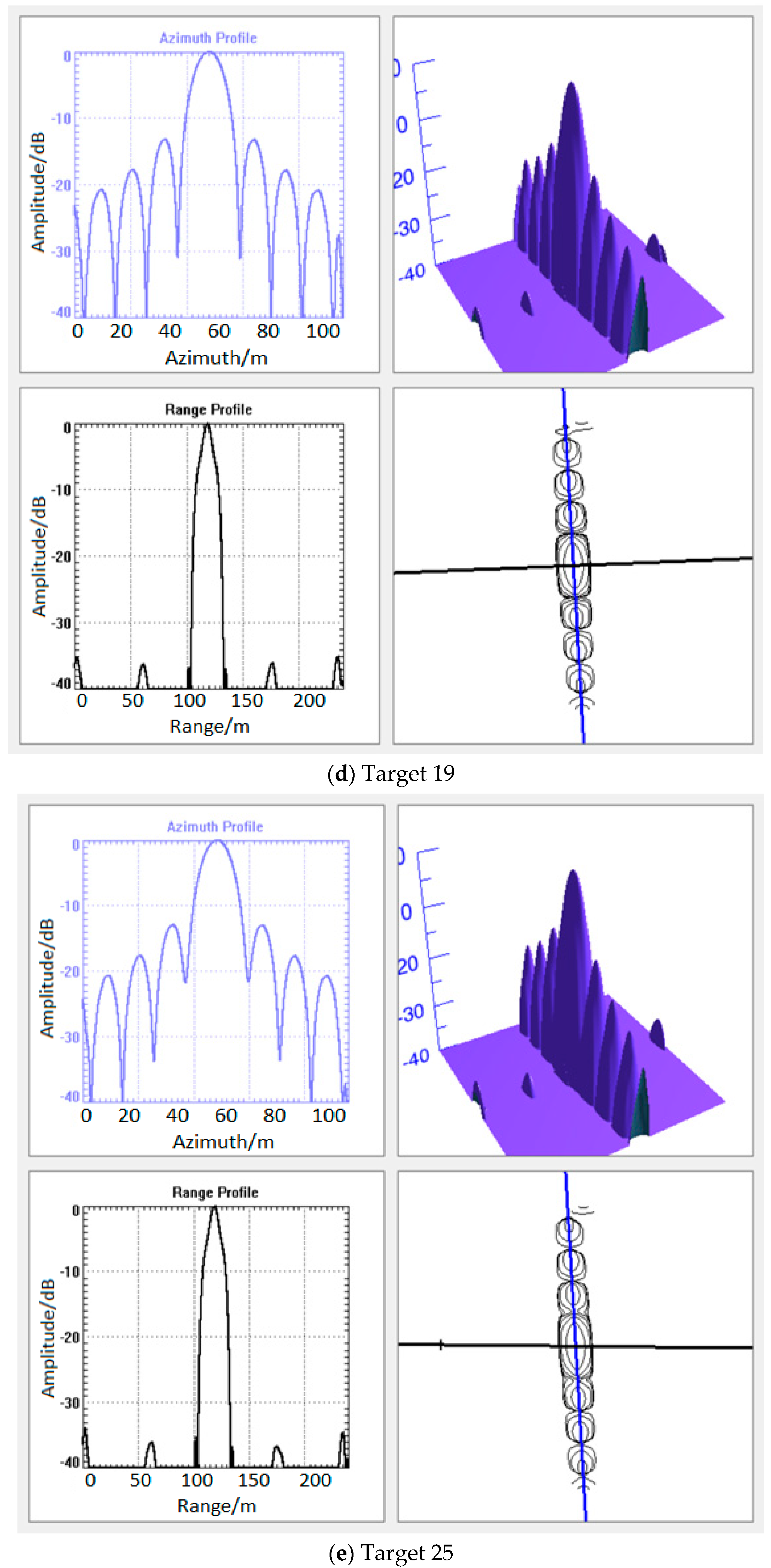
3.1. Simulation Results
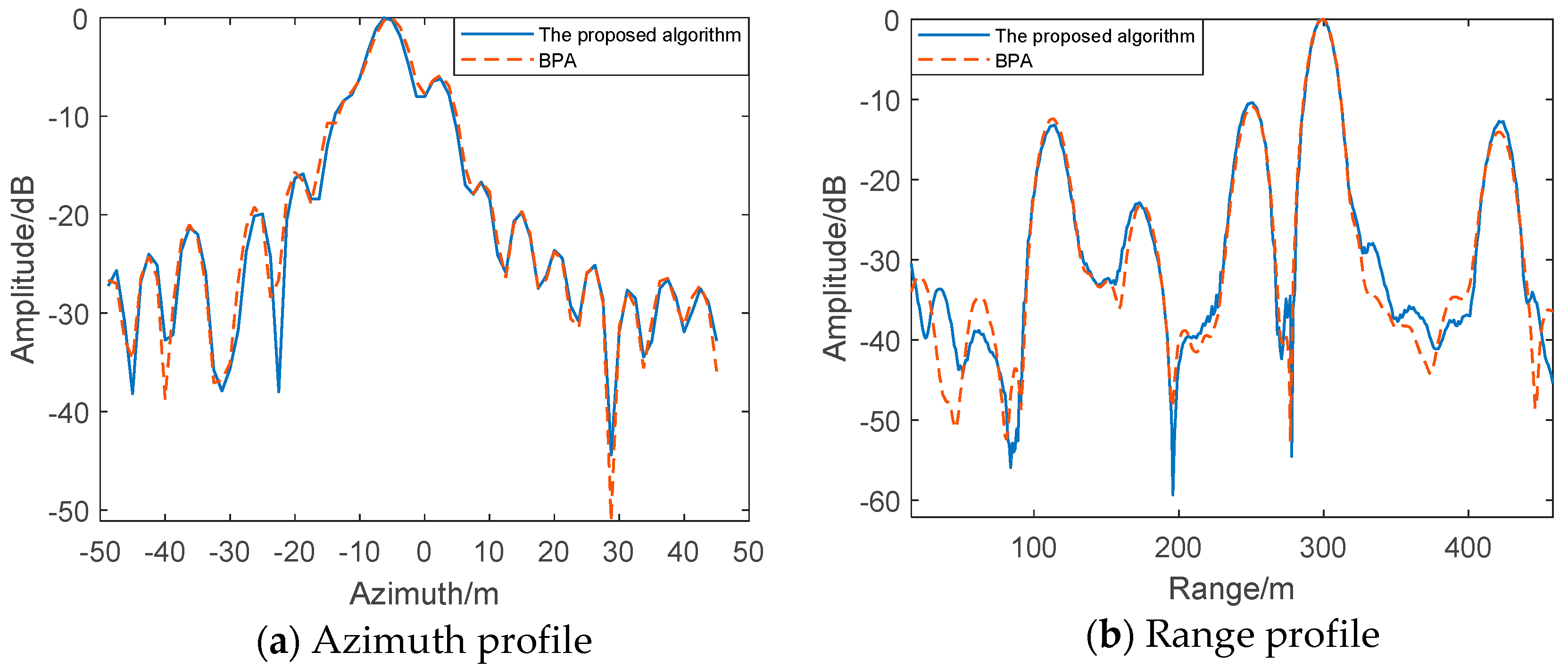
3.2. Experimental Results
4. Discussion
5. Conclusions
Author Contributions
Funding
Acknowledgments
Conflicts of Interest
References
- Foti, G.; Gommenginger, C.; Jales, P. Spaceborne GNSS reflectometry for ocean winds: First results from the UK TechDemoSat-1 mission. Geophys. Res. Lett. 2015, 42, 5435–5441. [Google Scholar] [CrossRef]
- Clarizia, M.P.; Ruf, C.S.; Jales, P. Spaceborne GNSS-R Minimum Variance Wind Speed Estimator. IEEE Trans. Geosci. Remote Sens. 2014, 52, 6829–6843. [Google Scholar] [CrossRef]
- Rodriguez-Alvarez, N.; Camps, A.; Vall-llossera, M. Land Geophysical Parameters Retrieval Using the Interference Pattern GNSS-R Technique. In Proceedings of the IEEE International Geoscience and Remote Sensing Symposium, Cape Town, South Africa, 12–17 July 2009; Volume 49, pp. 71–84. [Google Scholar]
- Rodriguez-Alvarez, N.; Bosch-Lluis, X.; Camps, A. Soil Moisture Retrieval Using GNSS-R Techniques: Experimental Results over a Bare Soil Field. In Proceedings of the IEEE International Geoscience and Remote Sensing Symposium, Boston, MA, USA, 7–11 July 2009; Volume 47, pp. 3616–3624. [Google Scholar]
- Egido, A.; Paloscia, S.; Motte, E. Airborne GNSS-R Polarimetric Measurements for Soil Moisture and Above-Ground Biomass Estimation. IEEE J. Sel. Top. Appl. Earth Obs. Remote Sens. 2014, 7, 1522–1532. [Google Scholar] [CrossRef]
- Ferrazzoli, P.; Guerriero, L.; Pierdicca, N. Forest biomass monitoring with GNSS-R: Theoretical simulations. Adv. Space Res. 2011, 47, 1823–1832. [Google Scholar] [CrossRef]
- Rius, A.; Nogues-Correig, O.; Ribo, S. Altimetry with GNSS-R interferometry: First proof of concept experiment. GPS Solut. 2012, 16, 231–241. [Google Scholar] [CrossRef]
- Cardellach, E.; Rius, A.; Martin-Neira, M. Consolidating the Precision of Interferometric GNSS-R Ocean Altimetry Using Airborne Experimental Data. IEEE Trans. Geosci. Remote Sens. 2014, 52, 4992–5004. [Google Scholar] [CrossRef]
- Hall, C.; Cordy, R. Multistatic scatterometry. In Proceedings of the IEEE International Geoscience and Remote Sensing Symposium, Edinburgh, UK, 12–16 September 1988; pp. 561–562. [Google Scholar]
- Martin-Neira, M. A passive reflectometry and interferometry system (PARIS): Application to ocean altimetry. Ecol. Soc. Am. J. 1993, 17, 331–355. [Google Scholar]
- Jin, S.; Cardellach, E.; Xie, F. GNSS Remote Sensing: Theory, Methods and Applications; Springer: Dordrecht, The Netherlands, 2014; Volume 19. [Google Scholar]
- Zavorotny, V.; Gleason, S.; Cardellach, E.; Camps, A. Tutorial on remote sensing using GNSS bistatic radar of opportunity. IEEE Geosci. Remote Sens. Mag. 2014, 2, 8–45. [Google Scholar] [CrossRef]
- Clarizia, M.P.; Gommenginger, C.P.; Gleason, S.T. Analysis of GNSS-R delay-Doppler maps from the UK-DMC satellite over the ocean. Geophys. Res. Lett. 2009, 36, L02608. [Google Scholar] [CrossRef]
- Ruf, C.S.; Gleason, S.; McKague, D.S. Assessment of CYGNSS Wind Speed Retrieval Uncertainty. IEEE J. Sel. Top. Appl. Earth Obs. Remote Sens. 2019, 12, 87–97. [Google Scholar] [CrossRef]
- Antoniou, M.; Cherniakov, M. GNSS-based bistatic SAR: A signal processing view. Eurasip J. Adv. Signal Process. 2013, 2013, 98. [Google Scholar] [CrossRef]
- Santi, F.; Pastina, D.; Bucciarelli, M.; Antoniou, M.; Tzagkas, D.; Cherniakov, M. Passive multistatic SAR with GNSS transmitters: Preliminary experimental study. In Proceedings of the European Radar Conference EuRAD, Rome, Italy, 8–10 October 2014; pp. 129–132. [Google Scholar]
- Cherniakov, M.; Saini, R.; Zuo, R.; Antoniou, M. Space-surface bistatic synthetic aperture radar with global navigation satellite system transmitter of opportunity-experimental results. IET Radar Sonar Navig. 2007, 1, 447–458. [Google Scholar] [CrossRef]
- Ma, H.; Antoniou, M.; Cherniakov, M. Passive GNSS-Based SAR Resolution Improvement Using Joint Galileo E5 Signals. IEEE Geosci. Remote Sens. Lett. 2015, 12, 1640–1644. [Google Scholar] [CrossRef]
- Santi, F.; Bucciarelli, M.; Pastina, D.; Antoniou, M.; Cherniakov, M. Spatial Resolution Improvement in GNSS-Based SAR Using Multistatic Acquisitions and Feature Extraction. IEEE Trans. Geosci. Remote Sens. 2016, 54, 6217–6231. [Google Scholar] [CrossRef]
- Santi, F.; Antoniou, M.; Pastina, D. Point Spread Function Analysis for GNSS-Based Multistatic SAR. IEEE Trans. Geosci. Remote Sens. 2015, 12, 304–308. [Google Scholar] [CrossRef]
- Santi, F.; Bucciarelli, M.; Pastina, D.; Antoniou, M. CLEAN technique for passive bistatic and multistatic SAR with GNSS transmitters. In Proceedings of the IEEE Radar Conference, Arlington, VA, USA, 10–15 May 2015; pp. 1228–1233. [Google Scholar]
- Liu, F.F.; Fan, X.Z.; Zhang, L.Z.; Zhang, T.; Liu, Q.H. GNSS-based SAR for urban area imaging: Topology optimization and experimental confirmation. Int. J. Remote Sens. 2019, 40, 4668–4682. [Google Scholar] [CrossRef]
- Liu, F.; Fan, X.; Zhang, T. GNSS-Based SAR Interferometry for 3-D Deformation Retrieval: Algorithms and Feasibility Study. IEEE Trans. Geosci. Remote Sens. 2018, 56, 5736–5748. [Google Scholar] [CrossRef]
- Zeng, H.-C.; Wang, P.-B.; Chen, J. A Novel General Imaging Formation Algorithm for GNSS-Based Bistatic SAR. Sensors 2016, 16, 294. [Google Scholar] [CrossRef]
- Zeng, T.; Liu, F.F.; Antoniou, M.; Cherniakov, M. GNSS-based BiSAR imaging using modified range migration algorithm. Sci. China Inf. Sci. 2015, 58, 1–13. [Google Scholar] [CrossRef]
- Gang, X. Principles of GPS and Receiver Design, 2nd ed.; House of Electronics Industry: Beijing, China, 2017; pp. 256–258. [Google Scholar]
- Wang, T.; Ruf, C.; Block, B.; McKague, D.; Gleason, S. Design and Performance of a GPS Constellation Power Monitor System for Improved CYGNSS L1B Calibration. IEEE J. Sel. Top. Appl. Earth Obs. Remote Sens. 2019, 12, 26–36. [Google Scholar] [CrossRef]
- Wong, F.H.; Cumming, I.G.; Neo, Y.L. Focusing bistatic SAR data using the nonlinear chirp scaling algorithm. IEEE Trans. Geosci. Remote Sens. 2008, 46, 2493–2505. [Google Scholar] [CrossRef]
- Wang, P.; Liu, W.; Chen, J. A High-Order Imaging Algorithm for High-Resolution Spaceborne SAR Based on a Modified Equivalent Squint Range Model. IEEE Trans. Geosci. Remote Sens. 2015, 53, 1225–1235. [Google Scholar] [CrossRef]
- Loffeld, O.; Nies, H.; Peters, V.; Knedlik, S. Models and useful relations for bistatic SAR processing. IEEE Trans. Geosci. Remote Sens. 2004, 42, 2031–2038. [Google Scholar] [CrossRef]
- Neo, Y.L.; Wong, F.; Cumming, I.G. A two-dimensional spectrum for bistatic SAR processing using series reversion. IEEE Geosci. Remote Sens. Lett. 2007, 4, 93–96. [Google Scholar] [CrossRef]
- Bamler, R.; Meyer, F.; Liebhart, W. No Math: Bistatic SAR Processing Using Numerically Computed Transfer Functions. In Proceedings of the IEEE International Geoscience and Remote Sensing Symposium, Denver, CO, USA, 31 July–4 August 2007; pp. 1844–1847. [Google Scholar]
- Qiu, X.L.; Hu, D.H.; Ding, C.B. A New Calculation Method of NuSAR for Translational Variant Bistatic SAR. In Proceedings of the IEEE International Geoscience and Remote Sensing Symposium, Cape Town, South Africa, 12–17 July 2010; pp. 296–299. [Google Scholar]
- Mittermayer, J.; Moreira, A.; Loffeld, O. Spotlight SAR data processing using the frequency scaling algorithm. IEEE Trans. Geosci. Remote Sens. 1999, 37, 2198–2214. [Google Scholar] [CrossRef]
- Moccia, A.; Renga, A. Spatial Resolution of Bistatic Synthetic Aperture Radar: Impact of Acquisition Geometry on Imaging Performance. IEEE Trans. Geosci. Remote Sens. 2011, 49, 3487–3503. [Google Scholar] [CrossRef]


| x | y | z | |
|---|---|---|---|
| Satellite position (km) | −5908 | −12,714 | 16,112 |
| Satellite velocity (m/s) | −2475 | −1198 | −1310 |
| Receiver position (m) | 0 | 0 | 6000 |
| Receiver velocity (m/s) | 60 | 0 | 0 |
| Satellite/Signal | GPS L5 |
|---|---|
| Carrier frequency | 1176.45 MHz |
| Signal bandwidth | 10.23 MHz |
| Sample rate | 40 MHz |
| Integration time | 10 s |
| Target | Range | Azimuth | ||||
|---|---|---|---|---|---|---|
| Resolution (m) | PSLR (dB) | ISLR (dB) | Resolution (m) | PSLR (dB) | ISLR (dB) | |
| 1 | 17.1 | −32.92 | −14.53 | 9.9 | −12.97 | −10.50 |
| 7 | 16.7 | −34.76 | −13.47 | 9.7 | −13.24 | −10.83 |
| 13 | 16.5 | −34.68 | −13.45 | 9.6 | −13.27 | −10.90 |
| 19 | 16.6 | −35.04 | −13.47 | 9.8 | −13.21 | −10.89 |
| 25 | 16.9 | −33.85 | −13.65 | 10.1 | −12.90 | −10.59 |
| Theoretical | 16.5 | −35.00 | −13.45 | 9.6 | −13.26 | −10.90 |
| Satellite used | GPS PRN30 |
| Signal used | L5 C/A code |
| Satellite elevation | 55.7° |
| Satellite azimuth | 268.6° |
| Carrier frequency | 1176.45 MHz |
| Sample rate | 62 MHz |
| Signal bandwidth | 10 MHz |
| Equivalent PRF | 1000 Hz |
| Doppler bandwidth | 151 Hz |
| x | y | z | ||
|---|---|---|---|---|
| Satellite position (km) | start | −11,822 | −300 | 17,341 |
| middle | −11,799 | − 735 | 17,341 | |
| end | −11,778 | −1172 | 17,332 | |
| Satellite velocity (m/s) | start | 173 | −3001 | −2 |
| middle | 137 | −2962 | −31 | |
| end | 129 | −2998 | −101 | |
| Na | Nr | Nx | Ny | Nkel |
|---|---|---|---|---|
| 3e5 | 1024 | 500 | 500 | 8 |
© 2019 by the authors. Licensee MDPI, Basel, Switzerland. This article is an open access article distributed under the terms and conditions of the Creative Commons Attribution (CC BY) license (http://creativecommons.org/licenses/by/4.0/).
Share and Cite
Zhou, X.-k.; Chen, J.; Wang, P.-b.; Zeng, H.-c.; Fang, Y.; Men, Z.-r.; Liu, W. An Efficient Imaging Algorithm for GNSS-R Bi-Static SAR. Remote Sens. 2019, 11, 2945. https://doi.org/10.3390/rs11242945
Zhou X-k, Chen J, Wang P-b, Zeng H-c, Fang Y, Men Z-r, Liu W. An Efficient Imaging Algorithm for GNSS-R Bi-Static SAR. Remote Sensing. 2019; 11(24):2945. https://doi.org/10.3390/rs11242945
Chicago/Turabian StyleZhou, Xin-kai, Jie Chen, Peng-bo Wang, Hong-cheng Zeng, Yue Fang, Zhi-rong Men, and Wei Liu. 2019. "An Efficient Imaging Algorithm for GNSS-R Bi-Static SAR" Remote Sensing 11, no. 24: 2945. https://doi.org/10.3390/rs11242945
APA StyleZhou, X.-k., Chen, J., Wang, P.-b., Zeng, H.-c., Fang, Y., Men, Z.-r., & Liu, W. (2019). An Efficient Imaging Algorithm for GNSS-R Bi-Static SAR. Remote Sensing, 11(24), 2945. https://doi.org/10.3390/rs11242945