Spectral Diversity Successfully Estimates the α-Diversity of Biocrust-Forming Lichens

 ,
,  , and
, and 
Abstract
1. Introduction
2. Materials and Methods
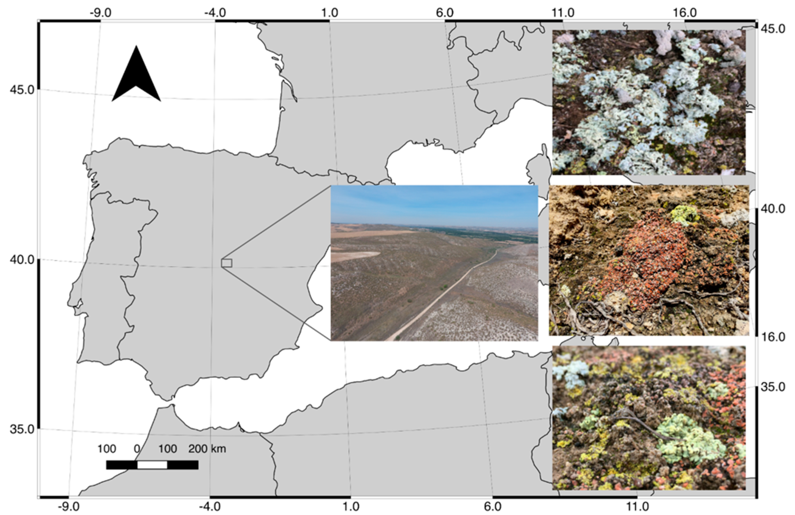
2.1. Study Area and Sampling
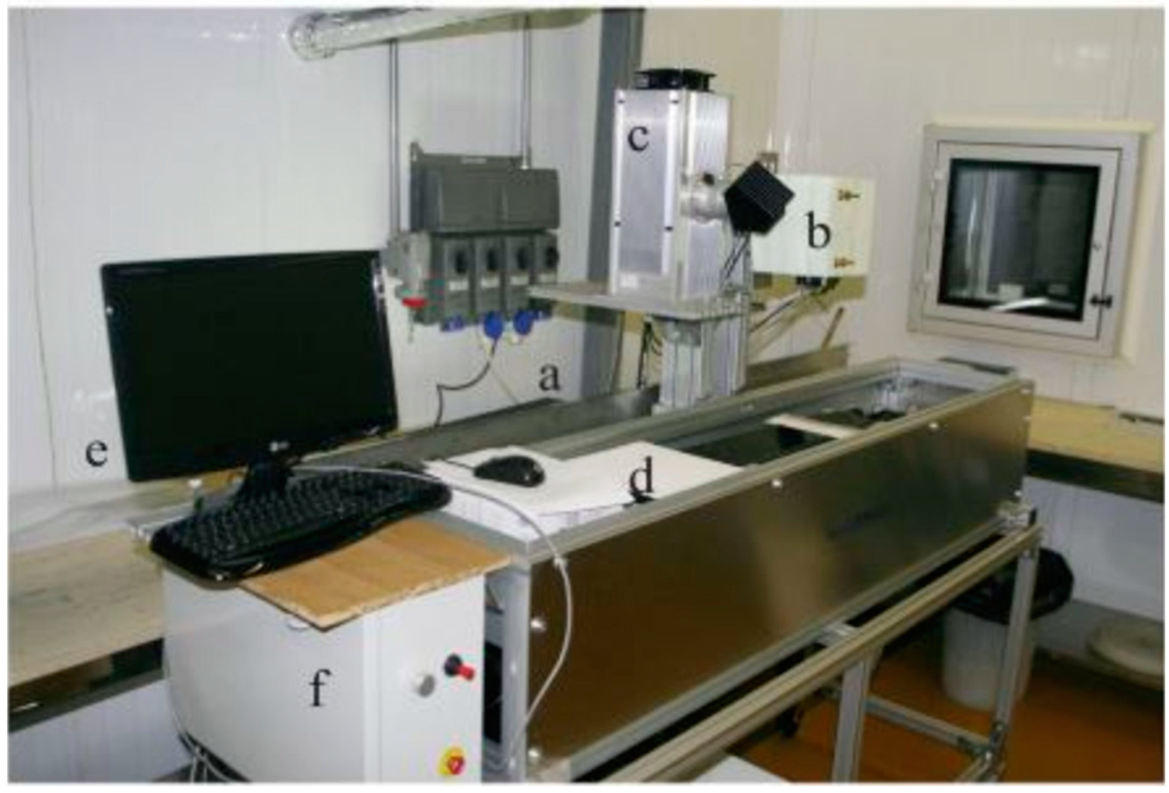
2.2. Hyperspectral Imagery Acquisition
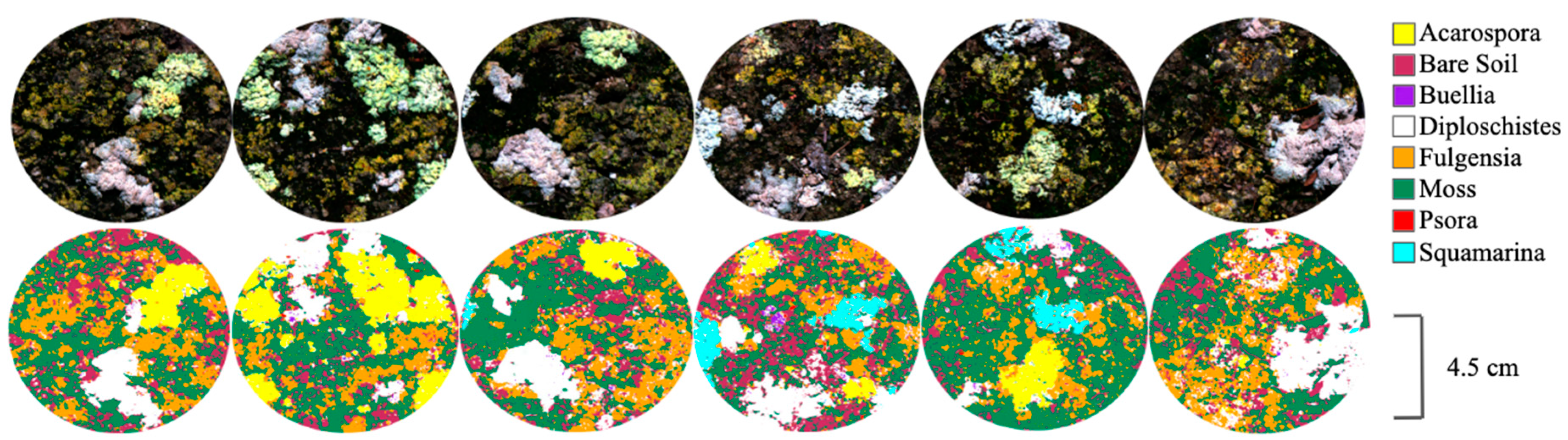
2.3. Images Processing and Classification
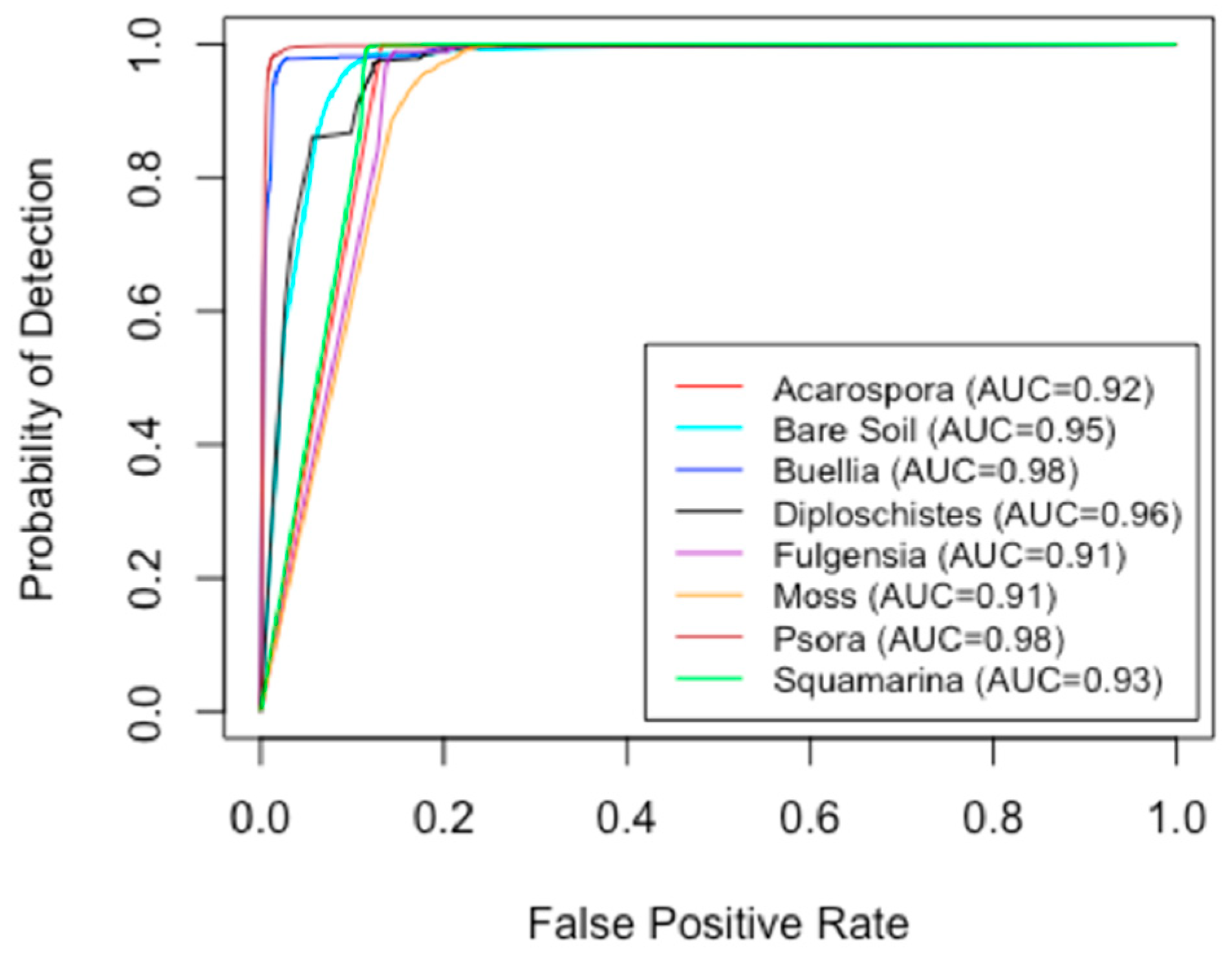
2.4. Validation of Classifications
2.5. Computation of the Spectral Diversity
2.6. Biodiversity Metrics
2.7. Statistical Analysis
3. Results
3.1. Classifications and Accuracy Evaluation
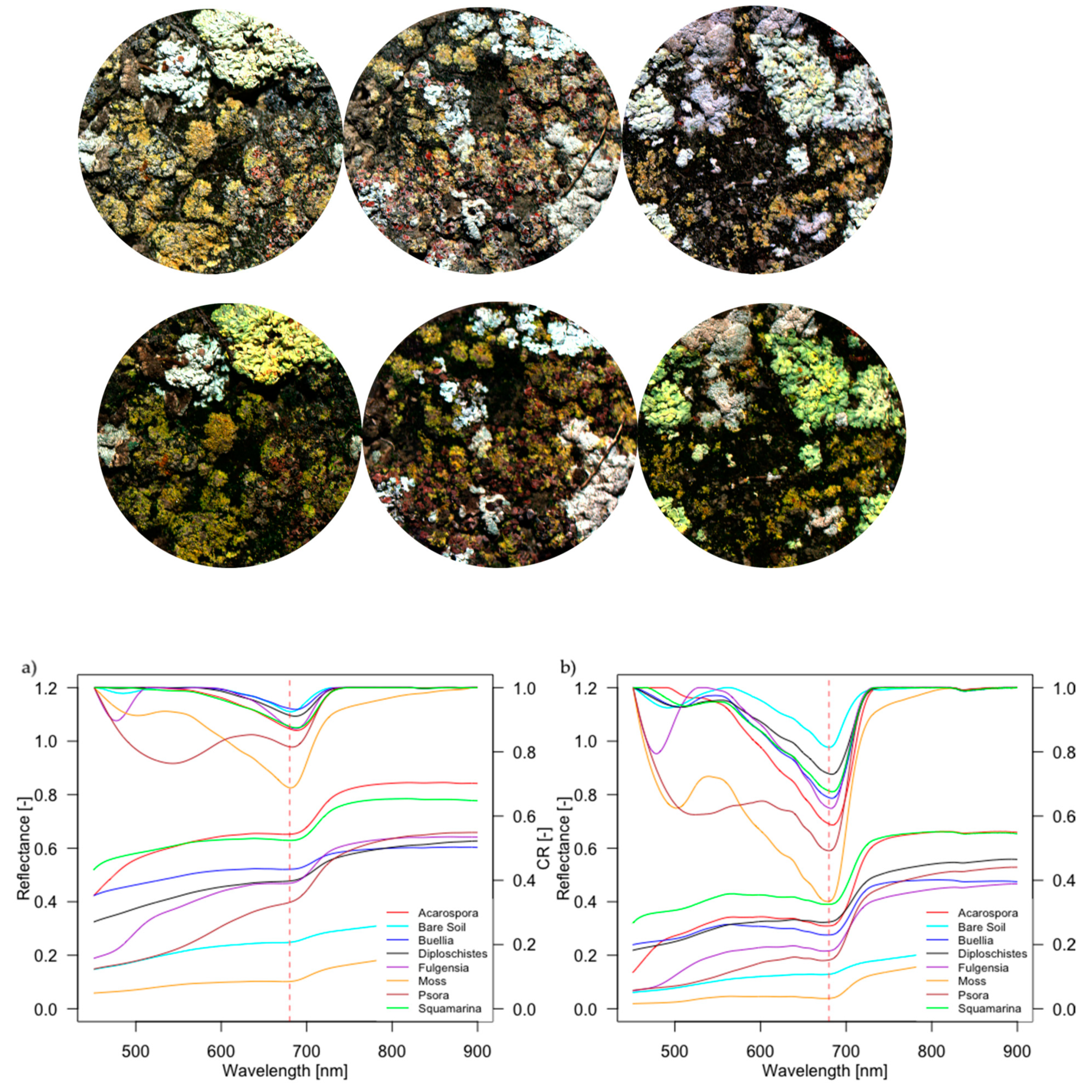
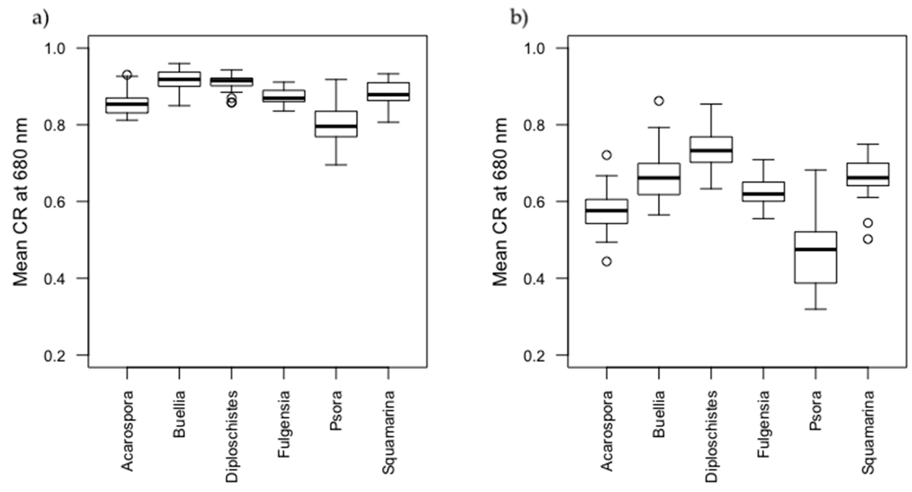
3.2. Spectral Characterization of Biocrusts
3.3. Fractional Cover of Biocrusts and Diversity Metrics
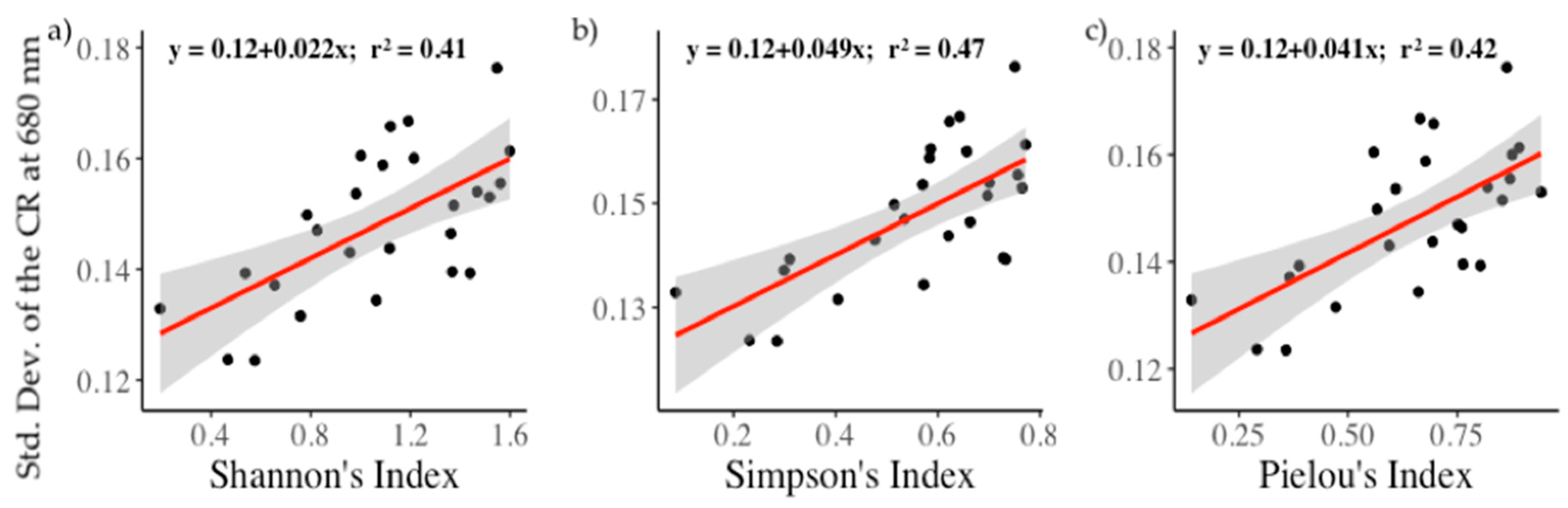
3.4. Relationships between Biodiversity and Spectral Diversity
4. Discussion
5. Conclusions
Author Contributions
Funding
Acknowledgments
Conflicts of Interest
References
- Belnap, J.; Lange, O.L. Biological Soil Crusts: Structure, Function, and Management; Springer Science & Business Media: Berlin, Germany, 2003; p. 150. [Google Scholar]
- Weber, B.; Büdel, B.; Belnap, J. Biological Soil Crusts: An Organizing Principle in Drylands, 1st ed.; Weber, B., Büdel, B., Belnap, J., Eds.; Ecological Studies; Springer: Berlin, Germany, 2016; Volume 226. [Google Scholar]
- Rodríguez-Caballero, E.; Castro, A.J.; Chamizo, S.; Quintas-Soriano, C.; Garcia-Llorente, M.; Cantón, Y.; Weber, B. Ecosystem services provided by biocrusts: From ecosystem functions to social values. J. Arid Environ. 2018, 159, 45–53. [Google Scholar] [CrossRef]
- Bowker, M.A.; Mau, R.L.; Maestre, F.T.; Escolar, C.; Castillo-Monroy, A.P. Functional profiles reveal unique roles of various biological soil crust organisms in Spain. Funct. Ecol. 2011, 25, 787–795. [Google Scholar] [CrossRef]
- Bowker, M.A.; Maestre, F.T.; Mau, R.L. Diversity and patch-size distributions of biological soil crusts regulate dryland ecosystem multifunctionality. Ecosystems 2013, 16, 923–933. [Google Scholar] [CrossRef]
- Bowker, M.A.; Maestre, F.T.; Escolar, C. Biological crusts as a model system for examining the biodiversity-ecosystem function relationship in soils. Soil Biol. Biochem. 2010, 42, 405–417. [Google Scholar] [CrossRef]
- Tongway, D.J.; Hindley, N. Landscape Function Analysis: Procedures for Monitoring and Assessing Landscapes; CSIRO Publishing: Brisbane, Australia, 2004; p. 82. [Google Scholar]
- Reed, S.C.; Maestre, F.T.; Ochoa-Hueso, R.; Kuske, C.R.; Darrouzet-Nardi, A.; Oliver, M.; Darby, B.; Sancho, L.G.; Sinsabaugh, R.L.; Belnaup, J. Biocrusts in the Context of Global Change. In Biological Soil Crust: An Organizing Principle in Drylands, 1st ed.; Weber, B., Büdel, B., Belnap, J., Eds.; Ecological Studies; Springer: Berlin, Germany, 2016; Volume 226, pp. 451–476. [Google Scholar]
- Rodríguez-Caballero, E.; Belnap, J.; Büdel, B.; Crutzen, P.J.; Andreae, M.O.; Pöschl, U.; Weber, B. Dryland photoautotrophic soil surface communities endangered by global change. Nat. Geosci. 2018, 11, 185–189. [Google Scholar] [CrossRef]
- Ferrenber, S.; Reed, S.C.; Belnap, J. Climate change and physical disturbance cause similar community shifts in biological soil crusts. Proc. Natl Acad. Sci. USA 2015, 112, 12116–12121. [Google Scholar] [CrossRef]
- Maestre, F.T.; Escolar, C.; Bardgett, R.D.; Dungait, J.A.J.; Gozalo, B.; Ochoa, V. Warming reduces the cover and diversity of biocrust-forming mosses and lichens, and increases the physiological stress of soil microbial communities in a semi-arid Pinus halepensis plantation. Front. Microbiol. 2015, 6, 865. [Google Scholar] [CrossRef]
- Ladrón de Guevara, M.; Gozalo, B.; Raggio, J.; Lafuente, A.; Prieto, M.; Maestre, F.T. Warming reduces the cover, richness and evenness of lichen-dominated biocrusts but promotes moss growth: Insights from an 8 yr experiment. New Phytol. 2018, 220, 811–823. [Google Scholar] [CrossRef]
- Bowker, M.A.; Eldridge, D.J.; Val, J.; Soliveres, S. Hydrology in a patterned landscape is co-engineered by soil-disturbing animals and biological crusts. Soil Biol. Biochem. 2013, 61, 14–22. [Google Scholar] [CrossRef]
- Delgado-Baquerizo, M.; Maestre, F.T.; Reich, P.B.; Jeffries, T.C.; Gaitán, J.J.; Encinar, D.; Berdugo, M.; Campbell, C.D.; Singh, B.K. Microbial diversity drives multifunctionality in terrestrial ecosystems. Nat. Commun. 2016, 7, 10541. [Google Scholar] [CrossRef]
- Nagendra, H. Using remote sensing to assess biodiversity. Int. J. Remote Sens. 2001, 22, 2377–2400. [Google Scholar] [CrossRef]
- Turner, W.; Spector, S.; Gardiner, N.; Fladeland, M.; Sterling, E.; Steininger, M. Remote sensing for biodiversity science and conservation. Trends Ecol. Evol. 2003, 18, 306–314. [Google Scholar] [CrossRef]
- Pettorelli, N.; Safi, K.; Turner, W.; Pettorelli, N. Satellite remote sensing, biodiversity research and conservation of the future. Philos. Trans. R. Soc. B 2014, 369, 20130190. [Google Scholar] [CrossRef] [PubMed]
- Rocchini, D.; Boyd, D.S.; Féret, J.B.; Foody, G.M.; He, K.S.; Lausch, A.; Nagendra, H.; Wegmann, M.; Pettorelli, N. Satellite remote sensing to monitor species diversity: Potential and pitfalls. Remote Sens. Ecol. Conserv. 2015, 2, 25–36. [Google Scholar] [CrossRef]
- Gillespie, T.W.; Foody, G.M.; Rocchini, D.; Giorgi, A.P.; Saatchi, S. Measuring and modelling biodiversity from space. Prog. Phys. Geogr. 2008, 32, 203–221. [Google Scholar] [CrossRef]
- Palmer, M.W.; Earls, P.; Hoagland, B.W.; White, P.S.; Wohlgemuth, T. Quantitative tools for perfecting species lists. Environmetrics 2002, 13, 121–137. [Google Scholar] [CrossRef]
- Schäfer, E.; Heiskanen, J.; Heikinheimo, V.; Pellikka, P. Mapping tree species diversity of a tropical montane forest by unsupervised clustering of airborne imaging spectroscopy data. Ecol. Indic. 2016, 64, 49–58. [Google Scholar] [CrossRef]
- Wang, R.; Gamon, J.A.; Emmerton, C.A.; Li, H.; Nestola, E.; Pastorello, G.Z.; Menzer, O. Integrated analysis of productivity and biodiversity in a southern Alberta prairie. Remote Sens. 2016, 8, 214. [Google Scholar] [CrossRef]
- Aneece, I.P.; Epstein, H.; Lerdau, M. Correlating species and spectral diversities using hyperspectral remote sensing in early-successional fields. Ecol. Evol. 2017, 7, 3475–3488. [Google Scholar] [CrossRef]
- Wang, R.; Gamon, J.A.; Cavender-Bares, J.; Townsend, P.A.; Zygielbaum, A.I. The spatial sensitivity of the spectral diversity-biodiversity relationship: An experimental test in a prairie grassland. Ecol. Appl. 2018, 28, 541–556. [Google Scholar] [CrossRef]
- Wang, R.; Gamon, J.A.; Schweiger, A.K.; Cavender-Bares, J.; Townsend, P.A.; Zygielbaum, A.I.; Kothari, S. Influence of species richness, evenness, and composition on optical diversity: A simulation study. Remote Sens. Environ. 2018, 211, 218–228. [Google Scholar] [CrossRef]
- Rocchini, D.; Balkenhol, N.; Carter, G.A.; Foody, G.M.; Gillespie, T.W.; He, K.S.; Kark, S.; Levin, N.; Lucas, K.; Luoto, M.; et al. Remotely sensed spectral heterogeneity as a proxy of species diversity: Recent advances and open challenges. Ecol. Inform. 2010, 5, 318–329. [Google Scholar] [CrossRef]
- Gholizadeh, H.; Gamon, J.A.; Zygielbaum, A.I.; Wang, R.; Schweiger, A.K.; Cavender-Bares, J. Remote sensing of biodiversity: Soil correction and data dimension reduction methods improve assessment of α-diversity (species richness) in prairie ecosystems. Remote Sens. Environ. 2018, 206, 240–253. [Google Scholar] [CrossRef]
- Karnieli, A. Development and implementation of spectral crust index over dune sands. Int. J. Remote Sens. 1997, 18, 1207–1220. [Google Scholar] [CrossRef]
- Chen, J.; Yuan Zhang, M.; Wang, L.; Shimazaki, H.; Tamura, M. A new index for mapping lichen-dominated biological soil crusts in desert areas. Remote Sens. Environ. 2005, 96, 165–175. [Google Scholar] [CrossRef]
- Weber, B.; Olehowski, C.; Knerr, T.; Hill, J.; Deutschewitz, K.; Wessels, D.C.J.; Eitel, B.; Büdel, B. A new approach for mapping of Biological Soil Crusts in semidesert areas with hyperspectral imagery. Remote Sens. Environ. 2008, 112, 2187–2201. [Google Scholar] [CrossRef]
- Rodríguez-Caballero, E.; Escribano, P.; Cantón, Y. Advanced image processing methods as a tool to map and quantify different types of biological soil crust. ISPRS J. Photogramm. Remote Sens. 2014, 90, 59–67. [Google Scholar] [CrossRef]
- Rozenstein, O.; Karnieli, A. Identification and characterization of Biological Soil Crusts in a sand dune desert environment across Israel–Egypt border using LWIR emittance spectroscopy. J. Arid Environ. 2015, 112, 75–86. [Google Scholar] [CrossRef]
- Panigada, C.; Tagliabue, G.; Zaady, E.; Rozenstein, O.; Garzonio, R.; Di Mauro, B.; De Amicis, M.; Colombo, R.; Cogliati, S.; Miglietta, F.; et al. A new approach for biocrust and vegetation monitoring in drylands using multi-temporal Sentinel-2 images. Prog. Phys. Geogr. 2019. [Google Scholar] [CrossRef]
- Waser, L.T.; Kuechler, M.; Schwarz, M.; Ivits, E.; Stofer, S.; Scheidegger, C. Prediction of lichen diversity in an UNESCO biosphere reserve—Correlation of high resolution remote sensing data with field samples. Environ. Model. Assess. 2007, 12, 315–328. [Google Scholar] [CrossRef]
- Weber, B.; Hill, J. Remote Sensing of Biological Soil Crusts at Different Scales. In Biological Soil Crust: An Organizing Principle in Drylands, 1st ed.; Weber, B., Büdel, B., Belnap, J., Eds.; Ecological Studies; Springer: Berlin, Germany, 2016; Volume 226, pp. 215–234. [Google Scholar]
- Ustin, S.L.; Valko, P.G.; Kefauver, S.C.; Santos, M.J.; Zimpfer, J.F.; Smith, S.D. Remote sensing of biological soil crust under simulated climate change manipulations in the Mojave Desert. Remote Sens. Environ. 2009, 113, 317–328. [Google Scholar] [CrossRef]
- Weksler, S.; Rozenstein, O.; Ben-Dor, E. Mapping Surface Quartz Content in Sand Dunes Covered by Biological Soil Crusts Using Airborne Hyperspectral Images in the Longwave Infrared Region. Minerals 2018, 8, 318. [Google Scholar] [CrossRef]
- Rodríguez-Caballero, E.; Paul, M.; Tamm, A.; Caesar, J.; Büdel, B.; Escribano, P.; Hill, J.; Weber, B. Biomass assessment of microbial surface communities by means of hyperspectral remote sensing data. Sci. Total Environ. 2017, 586, 1287–1297. [Google Scholar] [CrossRef] [PubMed]
- Lehnert, L.; Jung, P.; Obermeier, W.; Büdel, B.; Bendix, J. Estimating Net Photosynthesis of Biological Soil Crusts in the Atacama Using Hyperspectral Remote Sensing. Remote Sens. 2018, 10, 891. [Google Scholar] [CrossRef]
- Román, J.R.; Rodríguez-Caballero, E.; Rodríguez-Lozano, B.; Roncero-Ramos, B.; Chamizo, S.; Águila-Carricondo, P.; Cantón, Y. Spectral Response Analysis: An Indirect and Non-Destructive Methodology for the Chlorophyll Quantification of Biocrusts. Remote Sens. 2019, 11, 1350. [Google Scholar] [CrossRef]
- Clark, R.N.; Roush, T.L. Reflectance spectroscopy. Quantitative analysis techniques for remote sensing applications. J. Geophys. Res. 1984, 89, 6329–6340. [Google Scholar] [CrossRef]
- Rees, W.G.; Tutubalina, O.V.; Golubeva, E.I. Reflectance spectra of subarctic lichens between 400 and 2400 nm. Remote Sens. Environ. 2004, 90, 281–292. [Google Scholar] [CrossRef]
- Cano-Díaz, C.; Mateo, P.; Muñoz, M.A.; Maestre, F.T. Diversity of biocrust- forming cyanobacteria in a semiarid gypsiferous site from central Spain. J. Arid Environ. 2018, 151, 83–89. [Google Scholar] [CrossRef]
- Maestre, F.T.; Escolar, C.; Ladrón de Guevara, M.; Quero, J.L.; Lázaro, R.; Delgado-Baquerizo, M.; Ochoa, V.; Bergudo, M.; Gozalo, B.; Gallardo, A. Changes in biocrust cover drive carbon cycle responses to climate change in drylands. Glob. Chang. Biol. 2013, 19, 3835–3847. [Google Scholar] [CrossRef]
- Garzonio, R.; Di Mauro, B.; Cogliati, S.; Rossini, M.; Panigada, C.; Delmonte, B.; Maggi, V.; Colombo, R. A novel hyperspectral system for high resolution imaging of ice cores: Application to light-absorbing impurities and ice structure. Cold Reg. Sci. Technol. 2018, 155, 47–57. [Google Scholar] [CrossRef]
- Savitzky, A.; Golay, M.J.E. Smoothing and differentiation of data by simplified least squares procedures. Anal. Chem. 1964, 36, 1627–1639. [Google Scholar] [CrossRef]
- Cortes, C.; Vapnik, V. Support-Vector Networks. Mach. Learn. 1995, 297, 273–297. [Google Scholar] [CrossRef]
- Vapnik, B.V. Universal Learning Technology: Support Vector Machines. J. Adv. Technol. 2005, 2, 137–144. [Google Scholar]
- Foody, G.M.; Mathur, A.; Sanchez-Hernandez, C.; Boyd, D.S. Training set size requirements for the classification of a specific class. Remote Sens. Environ. 2006, 104, 1–14. [Google Scholar] [CrossRef]
- Chang, C.; Lin, C. LIBSVM: A library for support vector machines. ACM Trans. Intell. Syst. Technol. 2011, 2. [Google Scholar] [CrossRef]
- DeLeo, J.M. Receiver operating characteristic laboratory (ROCLAB): Software for developing decision strategies that account for uncertainty. In Proceedings of the 1993 (2nd) International Symposium on Uncertainty Modeling and Analysis, College Park, MD, USA, 25–28 April 1993; IEEE. Computer Society Press: College Park, MD, USA, 1993; pp. 318–325. [Google Scholar]
- Bradlye, A.P. The use of the area under the ROC curve in the evaluation of machine learning algorithms. Pattern Recognit. 1997, 30, 1145–1159. [Google Scholar] [CrossRef]
- Hanley, J.A.; McNeil, B.J. The meaning and use of the area under a receiver operating characteristic (ROC) curve. Radiology 1982, 143, 29–36. [Google Scholar] [CrossRef]
- Fawcett, T. An Introduction to ROC Analysis. Pattern Recognit. Lett. 2006, 27, 861–874. [Google Scholar] [CrossRef]
- Signorell, A.; Aho, K.; Alfons, A.; Anderegg, N.; Aragon, T.; Arppe, A.; Baddeley, A.; Barton, K.; Bolker, B.; Borchers, H.W.; et al. DescTools: Descriptive Tools Analysis. R Package Version 3.6.1 (R Foundation for Statistical Computing, Vienna). Available online: https://cran.r-project.org/web/packages/DescTools/index.html (accessed on 16 May 2019).
- Congalton, R.G.; Green, K. Assessing the Accuracy of Remotely Sensed Data: Principles and Practices, 2nd ed.; CRC Press, Taylor and Francis Group: London, UK, 2008. [Google Scholar]
- Shannon, C.E. A mathematical theory of communication. Bell Syst. Tech. J. 1948, 27, 379–423. [Google Scholar] [CrossRef]
- Simpson, E.H. Measurement of diversity. Nature 1949, 163, 688. [Google Scholar] [CrossRef]
- Pielou, E.C. The measurement of diversity in different types of biological collections. J. Theor. Biol. 1966, 13, 131–144. [Google Scholar] [CrossRef]
- Oksanen, J.; Blanchet, F.G.; Kindt, R.; Legendre, P.; O’Hara, R.B.; Simpson, G.L.; Solymos, P.; Stevens, M.H.H.; Wagner, H. Vegan: Community Ecology Package. R Package Version 2.4-5 (R Foundation for Statistical Computing, Vienna). 2017. Available online: https://CRAN. R-project.org/package=vegan (accessed on 15 June 2019).
- Gualtieri, J.A.; Cromp, R.F. Support vector machines for hyperspectral remote sensing classification. Proc. SPIE 1998, 3584, 221–232. [Google Scholar]
- Watanachaturaporn, P.; Arora, M.K.; Varshney, P.K. Hyperspectral image classification using support vector machines: A comparison with decision tree and neural network classifiers. In Proceedings of the American Society for Photogrammetry & Remote Sensing (ASPRS) 2005 Annual Conference, Reno, NV, USA, 7–11 March 2005. [Google Scholar]
- Plaza, A.; Benediktsson, J.A.; Boardman, J.W.; Brazile, J.; Bruzzone, L.; Camps-Valls, G.; Chanussot, J.; Fauvel, M.; Gamba, P.; Gualtieri, A.; et al. Recent advances in techniques for hyperspectral image processing. Remote Sens. Environ. 2009, 113, 110–122. [Google Scholar] [CrossRef]
- Ricotta, C.; Avena, G.C.; Volpe, F. The influence of principal component analysis on the spatial structure of a multispectral dataset. Int. J. Remote Sens. 1999, 20, 3367–3376. [Google Scholar]
- Stickler, C.M.; Southworth, J. Application of a multi-scale spatial and spectral analysis to predict primate occurrence and habitat associations in Kibale National Park, Uganda. Remote Sens. Environ. 2008, 112, 2170–2186. [Google Scholar] [CrossRef]
- Schweiger, A.K.; Cavender-Bares, J.; Townsend, P.A.; Hobbie, S.E.; Madritch, M.D.; Wang, R.; Tilman, D.; Gamon, J.A. Plant spectral diversity integrates functional and phylogenetic components of biodiversity and predicts ecosystem function. Nat. Ecol. Evol. 2018, 2, 976–982. [Google Scholar] [CrossRef]
- O’Neill, A.L. Reflectance spectra of microphytic soil crusts in semiarid Australia. Int. J. Remote Sens. 1994, 15, 675–681. [Google Scholar] [CrossRef]
- Karnieli, A.; Sarafis, V. Reflectance spectrophotometry of cyanobacteria within soil crusts—A diagnostic tool. Int. J. Remote Sens. 1996, 17, 1609–1614. [Google Scholar] [CrossRef]
- Chamizo, S.; Stevens, A.; Cantón, Y.; Miralles, I.; Domingo, F.; Van Wesemael, B. Discriminating soil crust type, development stage and degree of disturbance in semiarid environments from their spectral characteristics. Eur. J. Soil Sci. 2012, 63, 42–53. [Google Scholar] [CrossRef]
- Peet, R.K. The measurement of species diversity. Ann. Rev. Ecol. Syst. 1974, 5, 285–307. [Google Scholar] [CrossRef]
- Stohlgren, T.J.; Chong, G.W.; Kalkhan, M.A.; Schell, L.D. Multiscale sampling of plant diversity: Effects of minimum mapping unit size. Ecol. Appl. 1997, 7, 1064–1074. [Google Scholar] [CrossRef]
- Kalkhan, M.A.; Stafford, E.J.; Stohlgren, T.J. Rapid plant diversity assessment using a pixel nested plot design: A case study in Beaver Meadows, Rocky Mountain National Park, Colorado, USA. Divers. Distrib. 2007, 13, 379–388. [Google Scholar] [CrossRef]
- Kumar, S.; Simonson, S.; Stohlgren, T.J. Effects of spatial heterogeneity on butterfly species richness in Rocky Mountain National Park, CO, USA. Biodiv. Conserv. 2009, 18, 739–763. [Google Scholar] [CrossRef]
- Aasen, H.; Honkavaara, E.; Lucieer, A.; Zarco-Tejada, P. Quantitative remote sensing at ultra-high resolution with UAV spectroscopy: A review of sensor technology, measurement procedures, and data correction workflows. Remote Sens. 2018, 10, 1091. [Google Scholar] [CrossRef]
- Anderson, K.; Gaston, K.J. Lightweight unmanned aerial vehicles will revolutionize spatial ecology. Front. Ecol. Environ. 2013, 11, 138–146. [Google Scholar] [CrossRef]
- Somers, B.; Asner, G.P.; Tits, L.; Coppin, P. Endmember variability in Spectral Mixture Analysis: A review. Remote Sens. Environ. 2011, 115, 1603–1616. [Google Scholar] [CrossRef]
- Keshava, N.; Mustard, J.F. Spectral unmixing. IEEE Signal Proc. 2002, 19, 44–57. [Google Scholar] [CrossRef]


| α-Diversity Metric. | Formula |
|---|---|
| Species richness (S) | S = Number of classes |
| Shannon’s index (H’) | H′ = −∑pi ∗ ln (pi) |
| Reciprocal of Simpson’s index (D) | D = 1 / ∑pi 2 |
| Pielou’s index (J’) | J′ = H′ / ln (S) |
| Ground truth (%) | ||||||||
|---|---|---|---|---|---|---|---|---|
| Acarospora | Bare Soil | Buellia | Diploschistes | Fulgensia | Moss | Psora | Squamarina | |
| Acarospora | 99.96 | 0 | 0 | 0.04 | 0 | 0 | 0 | 0 |
| Bare soil | 0.04 | 97.55 | 0 | 0.72 | 0.4 | 0.32 | 1.06 | 0 |
| Buellia | 0 | 0 | 93.45 | 4.26 | 0 | 0 | 0 | 0.98 |
| Diploschistes | 0 | 1.63 | 6.49 | 94.89 | 0.24 | 0 | 1.3 | 0.23 |
| Fulgensia | 0 | 0.04 | 0 | 0 | 99.31 | 0 | 0.05 | 0 |
| Moss | 0 | 0.76 | 0 | 0 | 0.05 | 99.65 | 0.3 | 0 |
| Psora | 0 | 0.02 | 0 | 0 | 0.05 | 0.03 | 97.29 | 0 |
| Squamarina | 0 | 0 | 0.06 | 0.09 | 0 | 0 | 0 | 98.79 |
| Class | Samples | Plots | Mean Fc (%) | Max Fc (%) | Min Fc (%) | SD Fc (%) |
|---|---|---|---|---|---|---|
| Acarospora | 37 | 17 | 3.8 | 32.8 | 0.3 | 5.8 |
| Bare Soil | 54 | 18 | 21.6 | 46.1 | 5.1 | 8.1 |
| Buellia | 33 | 13 | 2.4 | 13.8 | 0.5 | 3 |
| Diploschistes | 54 | 18 | 14.6 | 53.1 | 0.1 | 11 |
| Fulgensia | 53 | 18 | 12 | 25.4 | 0.7 | 7.3 |
| Moss | 54 | 8 | 43.5 | 76.9 | 4.9 | 17 |
| Psora | 41 | 16 | 1.9 | 12.6 | 0.1 | 2.6 |
| Squamarina | 27 | 13 | 4.3 | 4.3 | 0.3 | 4.5 |
| α-Diversity Metric | SD_CR550–750 | SD_CR680 | CV420–900 | CV550–750 | CV680 |
|---|---|---|---|---|---|
| Species richness (S) | 0.001 | 0.003 | 0.005 | 0.013 | 0.08 |
| - | - | - | - | - | |
| Shannon’s Index (H’) | 0.012 | 0.022 | 0.056 | 0.063 | 0.071 |
| 0.33(0.001) | 0.41(0.0004) | - | - | 0.16(0.03) | |
| Simpson’s Index (D) | 0.02 | 0.049 | 0.156 | 0.164 | 0.184 |
| 0.39(0.0004) | 0.47(0.0001) | - | - | 0.26(0.007) | |
| Pielou’s Index (J’) | 0.023 | 0.041 | 0.112 | 0.118 | 0.141 |
| 0.39(0.0004) | 0.42(0.0002) | - | - | 0.19(0.02) |
| α-Diversity Metric | r2 | RMSE | rCV2 | RMSECV |
|---|---|---|---|---|
| Shannon’s index (H’) | 0.41 | 0.01 | 0.32 | 0.01 |
| Simpson’s index (D) | 0.47 | 0.009 | 0.39 | 0.01 |
| Pielou’s index (J’) | 0.42 | 0.009 | 0.35 | 0.01 |
© 2019 by the authors. Licensee MDPI, Basel, Switzerland. This article is an open access article distributed under the terms and conditions of the Creative Commons Attribution (CC BY) license (http://creativecommons.org/licenses/by/4.0/).
Share and Cite
Blanco-Sacristán, J.; Panigada, C.; Tagliabue, G.; Gentili, R.; Colombo, R.; Ladrón de Guevara, M.; Maestre, F.T.; Rossini, M. Spectral Diversity Successfully Estimates the α-Diversity of Biocrust-Forming Lichens. Remote Sens. 2019, 11, 2942. https://doi.org/10.3390/rs11242942
Blanco-Sacristán J, Panigada C, Tagliabue G, Gentili R, Colombo R, Ladrón de Guevara M, Maestre FT, Rossini M. Spectral Diversity Successfully Estimates the α-Diversity of Biocrust-Forming Lichens. Remote Sensing. 2019; 11(24):2942. https://doi.org/10.3390/rs11242942
Chicago/Turabian StyleBlanco-Sacristán, Javier, Cinzia Panigada, Giulia Tagliabue, Rodolfo Gentili, Roberto Colombo, Mónica Ladrón de Guevara, Fernando T. Maestre, and Micol Rossini. 2019. "Spectral Diversity Successfully Estimates the α-Diversity of Biocrust-Forming Lichens" Remote Sensing 11, no. 24: 2942. https://doi.org/10.3390/rs11242942
APA StyleBlanco-Sacristán, J., Panigada, C., Tagliabue, G., Gentili, R., Colombo, R., Ladrón de Guevara, M., Maestre, F. T., & Rossini, M. (2019). Spectral Diversity Successfully Estimates the α-Diversity of Biocrust-Forming Lichens. Remote Sensing, 11(24), 2942. https://doi.org/10.3390/rs11242942