Abstract
The detection of small fishing ships is very important for maritime fishery supervision. However, it is difficult to detect small ships using synthetic aperture radar (SAR), due to the weak target scattering and very small number of pixels. Polarimetric synthetic aperture radar (PolSAR) has been widely used in maritime ship detection due to its abundant target scattering information. In the present paper, a new ship detector, named ΛM, is developed based on the analysis of polarization scattering differences between ship and sea, then combined with the two-parameter constant false alarm rate method (TP-CFAR) algorithm to conduct ship detection. The goals of the detector construction are to fully consider the ship’s depolarization effect, and further amplify it through sliding window processing. First, the signal-to-clutter ratio (SCR) enhancement performance of ΛM for ships with different lengths ranging from 8 to 230 m under 90 different combinations of windows are analyzed in detail using three set of RADARSAT-2 quad-polarization data, then the appropriate window size is determined. In addition, the SCR enlargement between ΛM and some typical polarization features is compared. Among these, for ships of length greater than 35 m, the average contrast of ΛM is 33.7 dB, which is 20 dB greater than that of the HV channel. For small vessels of length less than 16 m, the average contrast of ΛM is 16 dB higher than that of HV channel on average. Finally, the RADARSAT-2 data including nonmetallic small vessels are used to perform ship detection tests, and the detection ability for conventional and small ships of some classic algorithms are compared and analyzed. For large vessels of length greater than 35 m, the method proposed in this paper is able to obtain a superior detection result, maintain the ship contour well, and suppress false alarms caused by the cross side lobe in the SAR image. For small vessels of length less than 16 m, the method proposed in this paper can reduce the number of missed targets, while also obtaining superior detection results, especially for small nonmetallic vessels.
1. Introduction
The monitoring of ships plays a significant role in shipping safety, fishery monitoring, maritime law enforcement, and combating illegal smuggling. As an important method of active detection, synthetic aperture radar (SAR) possesses the capabilities of penetrating clouds, avoiding the influence of light, and observing the Earth at all times and in all weather. For these reasons, it is widely applied in marine target monitoring such as ship detection.
As an artificial target, ships tend to produce strong backscatter echoes, which are highlighted in SAR images, while ocean background echoes are weak. SAR ship detection seeks to detect bright targets against a dark background, thus, the key of this matter is to determine the appropriate threshold at which to distinguish ship from sea. Obviously, the greater the difference is between them, the more favorable this will be for target detection. In general, signal-to-clutter ratio (SCR) can be used to describe the differences between ship and sea. Therefore, for both single-polarization SAR and multi-polarization SAR, ship detection mainly focuses on how to improve the SCR to achieve high-precision.
The constant false alarm rate (CFAR) method, which is based on sea clutter distribution, is the most widely used and classical method in ship detection for single-polarization SAR. The CFAR detection method is used adaptively to calculate the threshold value for separation between ship and sea based on the probability density function (pdf) of sea clutter in SAR images under the given false alarm rate. The common sea clutter pdf distribution models include K distribution [1], Gaussian distribution [2], lognormal distribution [3], generalized gamma distribution [4], and alpha-stable distribution [5]. Histogram fitting is used to select the appropriate distribution model. Generally speaking, each model has its own applicability for different resolutions, incidence angles, polarization modes, and sea conditions. Aside from the classical CFAR algorithm, in order to improve the detection performance of targets, researchers have developed several new detection algorithms by combining the CFAR method with other detection methods. For example, Leng et al. proposed a bilateral CFAR method that considers both pixel intensity and spatial distribution. Compared with ordinary CFAR, it is able to reduce the impact of sea clutter and SAR image ambiguity [6]. Schwegmann et al. proposed to convert the thresholds of cell average CFAR into diversified thresholds for different backgrounds, and conducted simulated annealing to select the appropriate threshold value for target detection combined with ship distribution [7]. Wang et al. proposed a ship detection algorithm by combining the feature analysis of ships and CFAR detector for high-resolution SAR images [8].
The application of PolSAR offers new opportunities for ship detection. There are mainly two kinds of methods for ship detection using PolSAR. The first, the polarimetric target decomposition method is used to distinguish ships from sea clutter. Wang et al. extracted the minimum eigenvalue of coherency T by Cloude decomposition, and used the local uniformity of the eigenvalue for ship detection [9]. Sugimoto et al. analyzed the differences of scattering mechanisms between ship and sea, then applied the Yamaguchi decomposition theory and CFAR method to achieve the goal [10]. Xi et al. developed a new four-component decomposition method based on the Yamaguchi decomposition theory, and defined a new detector using the component to ship detection [11]. Marino et al. developed a polarmatric notch filter for ship detection depending on the coherence of two scattering vectors [12,13]. By analyzing the scattering difference between ship and ocean, some new detectors that can significantly enhance the SCR were constructed using the polarization features, and many studies regarding these methods have been published. For example, Yang et al. constructed an objective function by combining similar parameters and energy terms, and solved the Generalized Optimization of Polarimetric Contrast Enhancement (GOPCE) issue to obtain a detector which enhanced the SCR, then carried out the CFAR method [14]. Shirvany et al. used the degree of polarization (DoP) parameter of compact polarization data to enhance the SCR and realize ship detection [15]. Touzi et al. constructed the optimal DoP by using the radar backscattering features, and this method exhibited a good enhancement effect on unstable ship targets [16]. Otherwise, some detectors that can distinguish ship and sea with a threshold of 0 were constructed using polarization features, and for such a detector, pixels in the detector with a value greater than 0 can be considered as the target, while those with a value less than 0 can be considered as the ocean [17].
In short, much research has been performed on SAR target detection, yet the current methods used have mainly been aimed at the detection of ordinary ships, while the detection of small ships, especially nonmetallic fishing boats and other small and weak targets, is rarely carried out. As shown by Marino’s research results, it is very difficult to detect small nonmetallic fishing boats (such as those of a fiberglass structure) in SAR images [12,13]. Even with the same structure, size, and other parameters, the Radar-Cross Section (RCS) of nonmetallic wooden fishing boats is typically much weaker than that of metal vessels [18]. Stastny et al. have conducted a SAR ship detection experiments with 6–25 m wooden ships, and found that even the ultrafine mode image of RADARSAT-2 with 3 m high-resolution could not provide reliable detection, and sometimes they could not even be detected [19]. In the research on SAR small ship detection, Arnaud proposed to detect small ship targets by using interferometric phase coherent graph [20], while Tello et al. proposed a method based on wavelet transform [21], and Ouchi et al. developed a method based on sub-look correlation [22]. In fact, both the wavelet and sub-look correlation methods require time-frequency decomposition, which will reduce the resolution of the image and weaken the small ship targets that only possess a small number of pixels, and render the detection more difficult. Gao proposed a target detection method using polarization notch filter for CFAR detection in heterogeneous sea clutter, which was further extended to the two-channel Along Track Interferometric SAR (ATI-SAR) mode. These methods were able to detect smaller ship targets [23,24]. However, there are currently no dual-channel ATI-SAR satellite data for ship monitoring. More recently, new algorithms based on deep learning were developed [25,26], but these require data base support, and the algorithm is complex, which also has high requirements for hardware systems.
There are currently more than 5 million fishing boats all over the world. The monitoring of fishing ships is of great significance for the development of local fisheries and ecological environment, but at present it is difficult to conduct surveillance on fishing vessels. For instance, China has the largest number of fishing boats in the world, with a total of more than 1.04 million as of the end of 2015. Among them, small fishing boats account for a very large proportion, and most are made of nonmetallic materials. If they do not install or turn on Automatic Identification System (AIS) devices, effective supervision cannot be achieved. Therefore, active detection methods are needed to detect small vessel targets, but conventional SAR ship detection methods may result in failure.
In fact, there are two reasons leading to the difficulty in detecting small ships. On one hand, small-sized ships are mostly nonmetallic fishing boats, and due to their material, simple structure, and the wobble of the target, it is difficult to form an effective strong scattering echo that is similar to that of an angle reflector. As a result, the vessels’ RCS is weak, sometimes at the same level as the ocean, thus rendering detection very difficult. For single polarimetric SAR, the target may be invisible in one polarization channel and tends to miss a greater number of targets [13,19]. On the other hand, regardless of whether the target is metal or not, due to the small number of pixels occupied by small-sized ships, it is easy to be regarded as speckle noise and filtered out in the detection process, particularly in the case of dense distribution of ships of different sizes.
PolSAR provides a wealth of scattering information regarding ships and oceans. If the scattering difference between ships and seas can be made use of, then a detector with high SCR performance can be constructed, which will be beneficial to the detection of small targets. In the present paper, the existing satellite PolSAR data were used to carry out research regarding small ship detection. On the basis of understanding the scattering characteristics of ship and sea, the depolarization effect of ships is fully considered and further amplified by sliding window processing. In addition, a ship detector based on PolSAR that can produce a large enhancement on SCR is proposed, and the ship detection is carried out by using the TP-CFAR.
The content of this paper is arranged as follows: Section 1 is the introduction; the principle of the new ship detector is introduced in Section 2; the data sources and the acquisition of SAR data for small vessels are described in Section 3; the influence parameters of the detector and enhancement performance are analyzed in Section 4; and the feasibility of the method through experimental data is verified in Section 5.
2. Target Detection Method Based on Scattering Difference for PolSAR
Constructing a detector with high SCR is an important way by which to improve the detection ability [14,16], especially for nonmetallic and small-sized ships with weak reflection echo. It is generally believed that the sea surface is Bragg scattering when space-borne SAR imaging the sea surface [27]. As an artificial target, the scattering pattern and mechanism of a ship are fundamentally different from those of the ocean. For cargo ships, containers, warships, and other large metal structure vessels, due to their complex structure and the influence of sea surface motion, the scattering of ship is complex, which mainly includes surface scattering on the surface of ships, double-bounce scattering caused by the hull’s structure, double-bounce scattering between ships and sea, and volume scattering and helix scattering caused by the complex superstructure of ships. Among these, the main scattering components of ships is double-bounce scattering [11,14,28]. However, for small-sized ships, especially the nonmetallic fishing boats, it is not easy to generate strong dihedral angle scattering if there is no obvious dihedral angle or trihedral angle reflector structure found on the ship. However, it can be considered that ships are mainly dominated by various types of depolarization energy. Fortunately, regardless of the situation, the total polarization scattering information of ship and sea surface can be obtained during PolSAR imaging. The polarization characteristics of the target can be fully expressed by the Sinclair matrix S [29], and here, the four matrix elements in Equation (1) represent the four polarization channel data:
On the basis of the S matrix, its second-order statistical characteristics coherency matrix T is then further extracted [27,30]:
Meanwhile, there is a corresponding relationship between the T matrix and Kennaugh matrix [29,31,32]:
The Kennaugh matrix can describe various backscattering mechanisms with polarization scattering power. The parameters in the Kennaugh matrix are known as Huynen parameters. In Equation (3), A0 represents the total scattered power from the regular, smooth, and convex parts of the scatterer; B0 + B represents the total symmetric or irregularity depolarized power; B0 – B represent the total nonsymmetric depolarized power; C and D represent the depolarization components of symmetric linear and curvature targets; E and F represent the depolarization components due to nonsymmetrical local twist torsion and helicity of target; and G and H represent the coupling terms between target’s symmetric and nonsymmetric terms [29,32].
According to the previous studies, |SHH + SVV|, |SHH – SVV|, and |SHV| correspond to the surface reflection (single-bounce scattering), and double-bounce reflection caused by the angular reflectors with direction angles of 0° and 45° [29]. In Equation (3), T11, T22, and T33, the three elements of T, respectively represent the surface scattering power and dihedral angular scattering power with an azimuth angle of 0° and 45°. As shown in Equation (3), T22 + T33 = 2B0 and T11 = 2A0. Here, A0 represents the total scattered power from the regular, smooth, and convex parts of the scatterer, while B0 denotes the total scattered power for the target’s irregular, rough, and nonconvex depolarizing components. The ship is dominated by double-bounce scattering, and the depolarization effect is strong, while the sea surface is dominated by Bragg scattering, and the depolarization effect is very weak [33,34]. In this way, since A0 contains the main energy of the ocean, and B0 contains almost all of the energy scattered by ships, the difference between A0 and B0 can be used to distinguish ship from ocean. Hajnsek et al. proposed the parameter M in Equation (4), which is independent of surface roughness, and is only related to the target dielectric constant and radar incidence angle [27]. Cloude carried out the trigonometric transformation on the M parameter, and dubbed it the Bragg angle ρB, which appears in Equation (5) [35]. Recently, Yin’s research showed that this parameter obtains good results in ship detection and oil spill detection [28].
For small-sized ships, the difference between ship and sea must be enhanced as much as possible in favor of target detection. How the two parameters A0 and B0 can be used to further improve the SCR must be considered. In this paper, we draw upon the work [18,36] to construct a new SCR enhanced detector ΛM, as shown in Equation (6), which considers the scattering difference between ship and sea in A0 and B0, and by means of the window sliding process, the scattering difference between ship and sea is further amplified. The detector is illustrated in Figure 1, and the entire training area is composed of the test area and background area. The training area in this paper is simply a parameter tuning approach and we just take the mean value of the pixels in the window for operation. The appropriate training window and test window must be selected to perform sliding window operation on the SAR image.
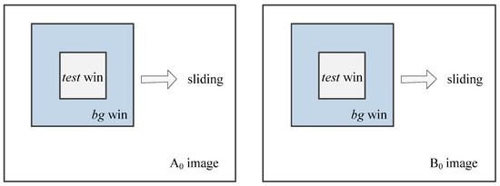
Figure 1.
Schematic diagram of window sliding for the ship detector.
Here, the symbols < >test and < >tr respectively represent the spatial average of the test and the training window area; test represents the test window; tr represents the training window; and bg represents the background window, where tr = bg + test. Here are some of the characteristics of ΛM:
- When the training window is sliding in a pure sea area, the pixels in the test window are relatively uniform, and the polarization power in both the test and training area basically remains unchanged. The numerator is close to 0, thus the ΛM is approximately 0.
- When a ship falls into the test window, the average B0 value in the test window must be larger than the surrounding background area, and the double-bounce scattering power of ships is larger than the single-bounce scattering in the test window, while the double-bounce scattering power of sea is lower than the single-bounce scattering in the background window. This will lead to the < B0 >test being a large value, while < B0 >tr and < A0 >tr are much smaller than < B0 >test, so that the detector ΛM will become large, and highlight the ship target.
- When the test window is on the edge of the ship, almost all of the pixels in the test window are oceans, while the background window contains ships. The < B0 >test will be smaller than < B0 >tr, so that the numerator may be negative, and likewise with ΛM.
In summary, the size of the test window is related to the size of the target that is to be tested, while the size of the training window depends on the detection accuracy that is sought to be achieved. Through the above analysis, the following conclusion can be obtained: when the sliding window processing is performed, if the target pixels fall into the test window, then the ΛM becomes a large value, and thus an image with very high SCR can be obtained for target detection.
According to the general process, the CFAR method is used to complete ship detection after the detector ΛM has been obtained. The CFAR method based on sea clutter distribution model requires accurate statistical modeling of sea background, which is time-consuming and difficult to achieve. In view of the large SCR of ΛM, the ΛM-based CFAR ship detection method in this paper no longer uses the complex clutter distribution modeling approach, and instead the TP-CFAR algorithm to complete the target detection [37]. The ship detection method process is shown in Figure 2. The sliding window processing is applied to the entire ΛM image, while the mean value mt, in the test window, and the mean value mb and variance value δb in the background window are calculated, respectively. When mt > t×mb + δb is satisfied, then the pixels in the test window are considered to be the real ship target. It can be seen that the detection algorithm mainly involves three parameters, namely the test window, training window, and CFAR threshold t. The setting of the window parameters will be analyzed in a later section of this paper.
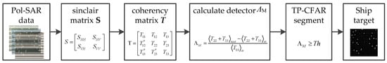
Figure 2.
Flowchart of ship detection method proposed in this paper.
3. Data
In this section, three quad-polarization RADARSAT-2 images with different beam modes are used for method verification, as shown in Figure 3, and the detailed information is shown in Table 1. Among them, the image acquired on 21 November 21 2015 is located in the Strait of Malacca, which contains a large number of ships, and synchronous AIS data are matched. In addition, two RADARSAT-2 quad-polarization SAR images containing small nonmetallic ships on 29 March 2015 and 2 August 2016 were obtained, and field optical photos, AIS, GPS, and other measured information were obtained at the same time. Four sub-images named #1–4 are selected to validate the SCR enhancement ability of the detector ΛM and the ship detection capability of the proposed method.
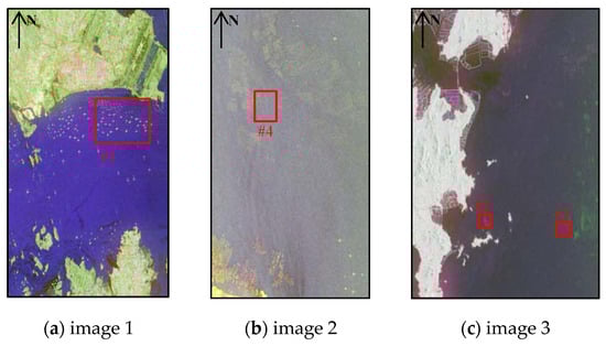
Figure 3.
PauliRGB images of RADARSAT-2 data acquired on (a) 21 November 2015, (b) 29 March 2015, and (c) 2 August 2016. The red box is the sub-image area used for following tests; several small vessels are included in sub-images #2, #3, and #4.

Table 1.
Detailed information of three synthetic aperture radar (SAR) images.
The SAR data acquired on 21 November 2015 shown in Figure 3a were taken from a location in the Strait of Malacca. The ships in the image had a complex distribution and had different lengths, ranging from 35 to 230 m, as determined by AIS verification. Samples were selected in this image for SCR enhancement analysis, and sub-image #1 (1600 × 1600), shown in Figure 4a, was used to test the detection performance for conventional large ships.
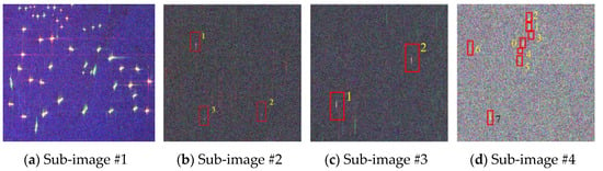
Figure 4.
Sub-images (a) #1, (b) #2, (c) #3, and (d) #4; the red boxes are small vessel targets, as determined by field data matching.
Figure 3c shows the data obtained through a field experiment in 2016. Three small fishing boats were used in this experiment, and the sub-image #2 (600 × 600) was extracted as shown in Figure 4c. The wind speed is 1.5–3 m/s, and the wind direction is northeasterly. It is a level-1 sea state according to the Beaufort scale, thus the sea surface is calm. Due to the fact that the sea area covered by this image is not a waterway, and it was in a fishing moratorium, the larger ships are not clearly visible. After matching with GPS information and distance correction, the locations of the three fishing boats were determined. Among them, Target 3 was anchored stationary (defined as ship_S), while the other two, Targets 1 and 2 ran at 5 knots along the range and azimuth direction (defined as ship_ R/A). An image of the ship is shown in Figure 5b. In addition, by analyzing the AIS base station information carried on the ship, two other ships in the nearby waters were matched and sub-image #3 (600 × 600) was extracted as shown in Figure 4d (defined as ship_1/2), and the length of both ships is 8 × 3 m. However, due to their far distance from the experimental area, the detailed information of type and structure of the two ships was not collected at the site. The SCR enhancement performance analysis of the small ships is mainly conducted using these two sub-images.
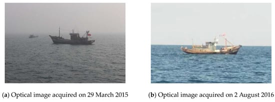
Figure 5.
Optical images of the small ships in each SAR image acquired on (a) 29 March 2015 and (b) 2 August 2016.
The SAR data collected on 29 March 2015 is shown in Figure 3b. After matching with the field optical photos as shown in Figure 5a and AIS data, the locations of small ships in this area were confirmed, and the sub-image was extracted and named #4 (600 × 600), as shown in Figure 4d. The Target 0 indicated in the image is a cement platform, on which there is steel house for storing equipment. Target 1 is a fishing boat, Targets 2 and 3 are foam float boats, and Targets 4 and 5 are wooden fishing boats, as determined with field optical photo verification, and Targets 6 and 7 are small ships by visual interpretation.
4. Parameter Setting and Enhanced Performance Analysis
4.1. Windows Parameter Test
From Equation (6) in Section 2, it can be seen that the size of test and training window will affect the enhancement performance of detector ΛM. In the present section, the RADARSAT-2 quad-polarization data were used to analyze the influence of these two window changes on the enhancement of the detector’s SCR.
According to the SAR image resolution, the pixels occupied by the ship are roughly determined, and the appropriate window can be set. Through the statistics of AIS data, the length of the ships is generally in the range of several tens of meters to 200 me, while the pixel spacing of the RADARSAT-2 quad-polarization SAR is about 4.8 × 4.7 m. Therefore, the range of the test window was set as 3 × 3 to 21 × 21, and the corresponding length of ship was about 15–100 m. When the test window was fixed, the background window gradually increased from 10 × 10 to 90 × 90, and the window setting rules are shown in Table 2.
Table 2.
Setting rules for test window and training window.
A series of ΛM detector images under different combinations of windows were calculated using the RADARSAT-2 data shown in Table 1. Several ship and sea samples were extracted from the ΛM images, and divided into six groups according to the ship length (220–230, 170–190, 90–110, 50–70, 35–45, and 8–16 m). Among these, the samples of ships longer than 35 m were selected from the images acquired on 21 November 2015 and each length interval includes 10 ships. The samples of ships length in the range of 8–16 m were selected from the other two images, and a total of 12 ships were used to calculate the average SCR of ΛM. Figure 6 shows the scatter plot of the detector ΛM with the changing window size. The vertical coordinate is the SCR (in dB), and the horizontal coordinate is the combination pair of different sized windows. The horizontal coordinates 1–9 correspond to a 3 × 3 test window, and the sizes of the training window are 13 × 13, 23 × 23...to 93 × 93. Additionally, the horizontal coordinates 10–18 correspond to a 5 × 5 test window, and the size of the training window is 15 × 15, 25 × 25...to 95 × 95, and so on. The different colors correspond to the six groups of ships.
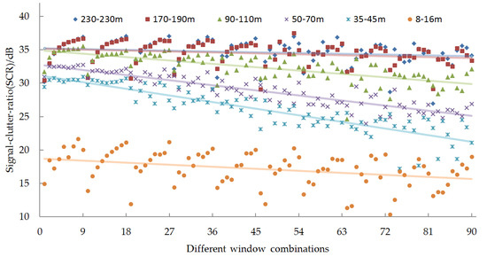
Figure 6.
Scatter plot of the detector ΛM under combination pairs of different sized windows. In the figure, the blue rhombus, red squares, green triangle, purple cross, blue snowflake, and yellow points indicate ships with length ranges of 220–230, 170–190, 90–110, 50–70, 35–4, and 8–16 m, respectively; the lines of a like color are the fitting lines based on least squares.
As shown in Figure 6, when the size of the test window is fixed and small (for example, 3 × 3 or 5 × 5), the SCR of ships with different lengths changes significantly. Taking the test window of 3 × 3 as an example, for ships with a length of greater than 90 m, the SCR gradually increases as the training window grows larger. Among these, for ships with a length of 90–110 m, the SCR is smaller when the training window is smaller than 23 × 23. However, when it is larger than 23 × 23, the SCR increases rapidly. This is because the smaller the test window is, the pixel of the ship will leak into the background window. At this time, the larger the background window is, the smaller the influence of the leaking pixel of ship on the background window will be, and the SCR will become larger with the increase of the background window. For ships with a length of 8–16 m, when the test window is fixed, the SCR changes dramatically when the background window increases. With small targets for which a larger SCR is desired, a small test window combined with a large background window is advantageous.
The lines in Figure 6 were obtained by the least squares fitting of these scatter points, which are then used to represent their change trend. It can be seen that when the test window is increased, the SCR of the different ship lengths tends to decrease. For large ships with a length of 170 m or more, the SCR is affected less significantly by the size of the test window, with only a slight decrease as the test window changes from 3 × 3 to 21 × 21. This is due to the large size of the ship, which may completely cover all sizes of test windows, while the background windows could average the pixels leaking into it. For vessels with a length range of 35–110 m, the SCR decreases significantly with the increase of test window. This is due to the fact that, with the increase of the test window, the pixels occupied by the ship in the test window gradually decrease, while the difference between the scattering power of the ship and sea in the test window and background window decrease. Consequently, the SCR naturally decreases too. For small ships with a length of less than 16 m, the SCR also decreases slightly as the test window changes, but the decline rate is slightly greater than that of the ships with a length of more than 170 m. This illustrates that the size of the test window is more sensitive to small vessel targets, while a small test window is more suitable for small target detection. In addition, it should be noted that in the SAR images, the ships with a length of 35–70 m are densely distributed. When the training window is large, some nearby ships fall into the background area and cause interference, thus leading to a low SCR of ΛM. However, if the ships are spaced far apart, the SCR of ΛM can be greatly improved. This can be simply summarized as follows: (1) the larger the length of the vessel is, the greater the SCR of ΛM will be; (2) the SCR gradually decreases as the test window becomes larger; (3) the larger the training window is, the greater the SCR will be when the test window is fixed.
Table 3 shows the statistical information of the detector ΛM for ships with a 3 × 3 test window. From the table it can be seen that the ΛM value of the sea area is steady, and the ΛM value of the ships increase gradually when the training window exceeds 23 × 23. The longer the ship length is, the larger the ΛM value will be, and the computing time also increased. Therefore, considering the SCR enhancement performance and time efficiency, the test window and training window being set to 3 × 3 and 43 × 43 is appropriate for the RADARSAT-2 quad polarization SAR data.
Table 3.
Mean statistical results of the detector ΛM when the test window is 3 × 3.
4.2. Performance Comparison for Different Polarization Features
The SCR enhancement performance of different polarization features, including the ΛM, SPAN, polarimetric whitening filter (PWF), B0 and HV, is compared in this section. The reasons for selecting these features are as follows: among the four channels of PolSAR, the cross-polarization HV channel has the greatest SCR for ship detection, the SPAN value contains the total energy of all channels, the PWF can effectively suppress the speckle noise without reducing the resolution, and B0 is a parameter of the method in this paper, which contains almost all the depolarized energy. Figure 7 shows the image of each feature. It can be seen from the figure that the sea clutter near the radar side is strong, and that the ship’s cross side lobe is obvious in the HV image. The target in the SPAN is stronger, but so is the sea clutter, thus the SCR enhancement is not obvious. The targets in the PWF and B0 are much stronger than the SPAN, and both also have strong cross side lobes. The target scattering is strong while sea clutters and cross side lobes around the ship are suppressed in ΛM, thus it is clear from the ΛM image that the SCR has been enhanced.
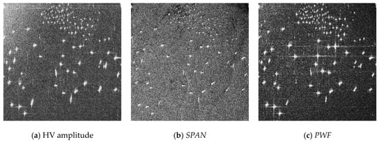
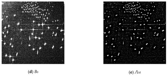
Figure 7.
Images of (a) HV amplitude, (b) SPAN, (c) polarimetric whitening filter (PWF), (d) B0, and (e) ΛM.
Figure 8 and Table 4 show the SCR curve and values of the HV, ΛM, B0, SPAN, and PWF features in terms of six different ship length groups. With the decrease in ship length, the SCR of ΛM, B0, and PWF attenuated gradually with a familiar trend. The SPAN and HV remain the same when the length is greater than 35 m, but the value of HV declines seriously when the length is less than 16 m. This may be due to the structure and material of small ship target leading to weak depolarization scattering in the HV channel, and better SCR can be obtained by using multipolarization information.
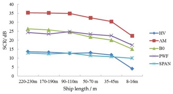
Figure 8.
Signal-to-clutter ratio (SCR) of HV, SPAN, B0, PWF, and ΛM for ships with different lengths.
Table 4.
Statistics for SCR of HV, SPAN, B0, PWF, and ΛM (unit: dB) for ships with different lengths.
The results of the data analysis show that ΛM has the largest SCR with 31.7 dB on average among the different ships. This is followed by B0 and PWF, with respective averages of 22.6 dB and 22.2 dB. The HV channel and SPAN are 11.4 dB and 11.7 dB, respectively, which are approximately the same. The order of the features is ΛM > PWF > B0 > SPAN > HV, and this applies for different lengths of ships. Compared with the HV, the SCR of ΛM were increased by 21.7, 21.9, 22.1, 19.5, 18.7, and 18.3 dB for the ships with different lengths. Therefore, it can be seen that the detector ΛM proposed in this paper is able to enhance the SCR very effectively, which is conducive to target detection.
4.3. SCR Enhancement Performance Analysis of Small Ships
The RADARSAT-2 data obtained on 2 August 2016 were used to analyze the visibility and SCR enhancement performances of small ships in detail. Figure 9 shows the σ0 image of each ship in four polarization channels, and the four lines from top to bottom, respectively, show the HH, HV, VH, and VV channels, while the five columns from left to right describe Ship_A, Ship_R, Ship_S, Ship_1, and Ship_2, respectively.
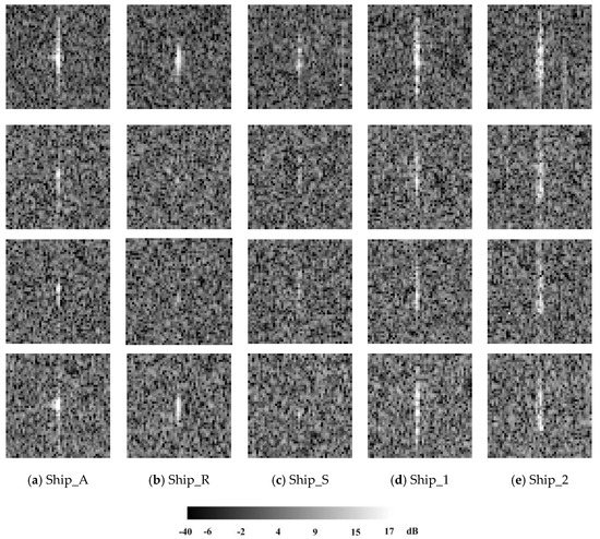
Figure 9.
RADARSAT-2 quad-polarization images of five small ships in four polarization channels.
In Figure 9, the five ships occupy fewer pixels in different polarization channels, resulting in poor visibility. With the exception of the Ship_A in the copolarization channel, the numbers of pixels occupied by the three small wooden fishing boats (Ship_A,Ship_R,Ship_S) were less than 20, while Ship_S and Ship_R were barely visible in the cross-polarization channel. Table 5 shows the SCR value of the five ships. In the copolarization channels, the order is Ship_A > Ship_R > Ship_S. In particular, Ship_A is 2–3 dB larger than Ship_R and 4–5 dB larger than Ship_S, while the HH channel has a stronger SCR. In the cross-polarization channel, the order is Ship_A > Ship_S > Ship_ R. In particular, Ship_A is 2 dB larger than Ship_S and 4–5 dB larger than Ship_R. In fact, both Ship_R and Ship_A were fitted with reflectors on their bows, which should produce a strong scattering intensity. However, these are not visible in the cross-polarization channel. A possible reason for this is that the interaction between the reflector and radar weakened the depolarization effect of ship during the SAR imaging process, while the radar energy is concentrated in the co-polarization channel. For Ship_1 and Ship_2, the SCR in the four channels is HH > HV > VH > VV, and the scattering intensity and SCR of the two ships are approximately the same in the co-polarization channel, with a deviation of only 0.5–1.4 dB.
Table 5.
SCR (dB) of the five small ships in RADARSAT-2 images acquired on 2 August 2016.
Detector ΛM was calculated using the method proposed in Section 2, and the test window and training window were set to 3 × 3 and 43 × 43. Figure 10 shows the HH, HV, and ΛM images of the two sub-images #2 and #3, it can be seen that the visibility of the ships has increased greatly in the ΛM images. Table 5 shows the intensity statistics of small the ships in sub-images #2 and #3, and the SCR of Ship_A in ΛM is 7.4, 12.9, and 10.3 dB larger than HH, HV, and VV, respectively; Ship_R in ΛM is 5.7, 12.6, and 9.3 dB larger than HH, HV, and VV, respectively; and Ship_S in ΛM is 16.1, 21, and 18.4 dB larger than HH, HV, and VV, respectively. Similarly, Ship_1 in ΛM is 13.2, 18.2, and 17.4 dB larger than HH, HV, and VV respectively; and Ship_2 in ΛM is 14, 18.6, and 17.1 dB larger than HH, HV, and VV respectively, so that the SCR of the small ships is greatly improved in ΛM, and the detectability of small ships has been significantly enhanced.
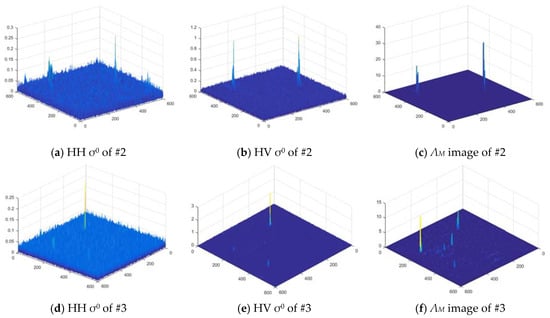
Figure 10.
(a) HH σ0, (b) HV σ0, and (c) ΛM 3D images of sub-image #2; (d) HH σ0, (e) HV σ0, and (f) ΛM 3D image of sub-image #3.
5. Ship Detection Performance Validation
In this section, the performance of the ship detection algorithm developed in this paper is validated. The classical CFAR algorithm based on the K distribution model on HV channel (HV-K), the SPAN method, PWF method [38], and Polarimetric Notch Filter (GNF) method [39] are used to perform comparisons. The SPAN method uses all of the energy of the four polarimetric channels to enhance the energy of the target. The PWF method suppresses the sea clutter speckle to obtain a speckle-reduced image by optimally combining the polarimetric data. The GNF method performs the target detection process in the polarimetric space, and suppresses the specific scattering mechanism, such as sea scattering, to highlight the target. For the HV-K method, the constant alarm rate is set to 0.001 to ensure the detection rate of the target. The SPAN and PWF methods also adopt the TP-CFAR algorithm for detection. While the threshold value t = 5–6 is generally recommended for intensity images [37], in this paper the threshold t was selected for the different method. For the SPAN method, t was set to 5 since the SCR is very close to the HV image, while for the PWF image with a higher SCR, t = 10 was adopted. For ΛM images, as the SCR of ΛM is many times greater than the HV, the threshold t was set to 15 to reduce the occurrence of false alarms. For the GNF method, the value a/b = 0.1, and the segmentation value was set to 0.9. Traditionally, background clutter pixels are removed by morphological filtering after detection. Small targets are present in the image to be detected. It is difficult to distinguish small targets from small false alarms caused by sea clutter. In order to evaluate the algorithm objectively, morphological filtering was not performed for any of the methods after the detection.
In order to comprehensively evaluate the ship detection performance of the proposed method, the quality factor FOM, which considers both the detection rate (PD) and false alarm rate (PFA) of the target, was used to evaluate the detection results [11]. The higher FOM is, the better the detection performance will be.
Here, Ntt is the number of correctly detected targets, Nfa is the number of false alarms caused by clutter or other factors, Nmt is the number of missed targets, and Ngt = Ntt + Nmt is the actual number of ships verified by ground truth. The red circle represents false alarm and the green triangle represents missed targets in the images.
5.1. Conventional Ship Detection Test
The SAR data acquired on 21 November 2015 was used to test the detection performance of ordinary ships. Sub-image #1 is located in the Strait of Malacca. The ships in this image had a complex distribution and different lengths. Through AIS verification, the orange rectangular trapezoid area in Figure 11a concentrates some of the ships with a length range of 35–70 m, while the remaining vessels in the figure have a length of 70–230 m. Figure 11b–f shows the detection results of these methods, the detection results of which will now be analyzed in detail. The HV-K method can detect all targets; in fact, under the condition of high-resolution data, the CFAR method can achieve very accurate detection for ordinary ships, and is fully applicable to the operational detection system [40]. The SPAN method can detect almost all targets, but there are many cases of target fracture in the results. In this paper, we still consider the fractured target as the same one, but in practical operation, these faults require further treatment to reduce the number of false alarms caused by this. Both the PWF and GNF methods generated several false alarms. The false alarms of the PWF method may have been caused by system noise. These system noises are mostly red points in the PauliRGB image, which indicates that it has strong energy in |HH-VV| and corresponds to the pixels with strong double-bounce scattering. The GNF method can significantly enhance the target, and some false alarms caused are the same as those caused by the PWF. In addition, this method lacks the inhibitory effect on the strong cross side lobe, and some residual side lobes are present around the detected target, which also caused false alarms. These cross side lobes are also mostly indicated by the red points in the PauliRGB image, corresponding to double-bounce scattering, which is consistent with the original design principle of the GNF ship detector. The method proposed in this paper performs well in terms of controlling the PD and PFA. In addition, it can eliminate the influence of the cross lobe and maintain the contour information in the detection results. The HV-K and GNF methods can detect all targets, while the other three methods all missed one target. This is because they do not adopt the global threshold segmentation, instead using a local TP-CFAR with a sliding window, which may result in targets being missed at a relatively close distance. Overall, these methods all exhibit good performance in the ordinary ship detection.
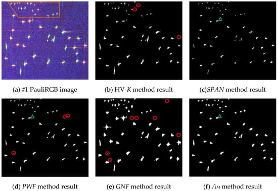
Figure 11.
(a) PauliRGB of sub-image #1 and detection results of the (b) HV-K, (c) SPAN, (d) PWF, (e) polarimetric notch filter (GNF), and (f) ΛM methods.
5.2. Small Ship Detection Test
Sub-images #2–#4 contain only small ship targets that have been verified by AIS and observed in the field. The length of all of the ships is less than 32 m, and most are less than 16 m. Next, the detection capability of the different methods for small vessels is compared. The detection results presented here are the best results obtained while considering the control of PD and PFA. Figure 12 shows the target detection results of small ships in region #2. All of the ships in this region are 16 × 4 m in size. For the HV-K method, the detection results show that only Ship_A is correctly detected, while both Ship_R and Ship_S are missed, which is due to the fact that these two targets are barely visible in the HV channel. The SPAN method detected Ship_R and Ship_A, but missed Ship_S. For the PWF method and the proposed method, all three ships are detected, but a false alarm target is also introduced, thus reducing the overall FOM. The method proposed in this paper shows strong detection capability for all three ships. It is unfortunate that the GNF method does not work at all in this image, and we attempted to explain this result. The GNF method considers the sea surface as Bragg scattering and target as other scattering components, then uses the polarimetric coherence technique in a six-dimensional polarization space to achieve sea clutter suppression and target enhancement. Due to the fact that the sea surface is relatively calm that day and the incident angle is relatively large (about 41°) during SAR imaging, under this condition the sea surface will not generate strong Bragg scattering and the scattering of sea surface is relatively random [41,42]. It is found that the scattering mechanism of the sea area in this image is not only Bragg scattering, but also contains many other scattering components such as double-bounce reflection, random surface and anisotropic particles by using the H-A-α decomposition [43]. Therefore, the sea clutter could not be effectively suppressed, but may have been enhanced by the GNF method, thus leading to failure in the detection.
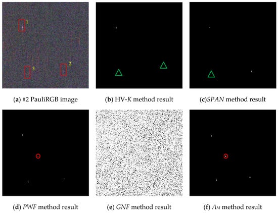
Figure 12.
(a) PauliRGB of sub-image #2 and detection results of the (b) HV-K, (c) SPAN, (d) PWF, (e) GNF, and (f) ΛM methods.
Figure 13 shows the target detection results of small ships in region #3. The ship geometry parameter in this image is 8 × 3 m. The vessel is smaller in size compared to that in sub-image #2, but is more visible and detectable due to its metal material and structure. It can be seen from Figure 13a that there is a strong clutter near ship_1. All of the targets were detected using our method, and the sea clutter was effectively suppressed. SPAN also shows a strong result. For the HV-K method, both ship targets were detected. However, multiple false alarms were also introduced, and the false alarm targets were almost connected into a line. For the sake of simplicity, this is regarded as a single false alarm. The clutter pixels causing false alarm are green in the PauliRGB image, which indicates that the clutter has a strong energy in the HV channel, thus, for the HV-K method, this clutter causes false alarm. Due to the fact that the small target is small and only consists of a small number of pixels, the conventional model-based CFAR method has no ability to suppress noise when clutter such as system noise exists, which has a serious impact on the detection of small targets. For the SPAN, PWF methods, and the method proposed in this paper, the clutter is effectively suppressed, and the target is detected.
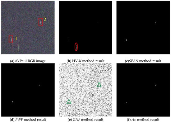
Figure 13.
(a) PauliRGB of sub-image #3 and detection results of the (b) HV-K, (c) SPAN, (d) PWF, (e) GNF, and (f) ΛM methods.
Figure 14 shows the detection results for sub-image #4. Compared with the previous sub-images, the sea condition in this image is higher and the ship target is not bright. As described in Section 3, in this sub-image, seven small ship targets and one small offshore platform can be considered as small targets. The size of the platform (in Figure 12a, position “0”) is about 20 × 10 m. It is fixed and there is a containerized house on the platform, thus the scattering is strong, and all methods can detect this target. Target 1 is a 32 × 6 m fishing boat, which has metal structures, and all of the methods are effective for the detection of this ship, which is consistent with the results in sub-image #1. Target 7 is similar to Target 1, thus, it can be detected by various methods. In addition, the HV-K and GNF methods caused the fracture of Target 7, which was detected as multiple targets. Targets 2 and 3 are foam float boats located near Target 1, while Targets 4–6 are also small ships. These smaller ships are not easily detected due to their smaller size and lower SCR. All of the methods miss a certain number of targets, among which, the SPAN method had the largest number of missed targets, while the method proposed in this paper only missed one ship. In comparison, the HV-K method, PWF method and GNF methods missed two, three, and four targets, respectively. Different from the previous two sub-images, the GNF method shows better detection ability for small ships in this image. It can be seen that Target 4 is missed by all methods, which is because it is very close to the other targets and the SCR is very low, thus, it is easy to miss when using either the local TP-CFAR or global CFAR method. Consequently, the method proposed in this paper can significantly enhance the SCR of the target, and improve the detectability of the small target.
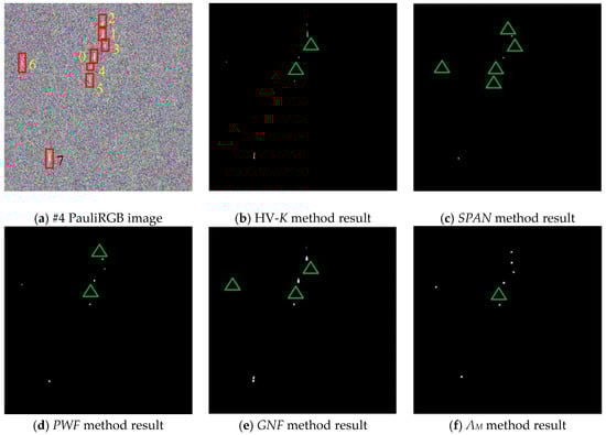
Figure 14.
(a) PauliRGB of sub-image #4 and detection results of the (b) HV-K, (c) SPAN, (d) PWF, (e) GNF, and (f) ΛM methods.
The detection results of the regular and small ships are listed in Table 6. There are 49 ships in #1, and among the many methods, the HV-K and GNF methods have the best detection ability, yet the GNF also introduced a greater number of false alarms, thus, leading to a low FOM. In fact, if morphological filtering is applied to the scene that contains the large ship targets, false alarms can be suppressed to some extent, and the FOM can be improved. There are 13 small targets in sub-images #2–#4 combined. The method proposed in this paper can achieve a high detection effect with a FOM of 0.85, while the FOM of the other classical methods are all less than 0.8. The results show that the method has advantages in small ship detection. The low FOM in small ship detection is mainly due to missed targets. If the segmentation threshold is lowered, then the PD can be increased, yet at the same time more false alarm targets will be introduced. The size of these false alarm targets is close to the real target, and it is very difficult to remove them.
Table 6.
Ship detection results of all four sub-images.
6. Conclusion and Discussion
The SAR detection of small ships such as fishing boats is not only difficult, it is also a topic of interest at present. Our experiments confirmed the visibility and detectability of the RADARSAT-2 quad-pol SAR data for small ships. If a ship is not visible in any of the four polarization channels, it will be hardly detectable or even undetectable in the image domain. In this paper, ships are visible in at least one SAR polarization channel, though they are small and occupy fewer pixels in the SAR image. From the perspective of the differences between depolarization power and total power, double-bounce scattering, and surface scattering, the parameters B0 and A0 were used to construct a new detector ΛM, which is able to significantly enhance the SCR, and is followed by the TP-CFAR method to complete ship detection. The conclusions of the study are as follows:
- (1)
- The effect of the window size on the SCR of the ΛM: the greater the length of the ship is, the greater the SCR enhancement of ΛM will be, and the SCR gradually decreases as the test window grows larger. However, when the test window is fixed, the larger the training window is, the larger the SCR will be. For RADARSAT-2 quad-polarization SAR with 8 m resolution, it is recommended to respectively set the test window and training window as 3 × 3 and 43 × 43.
- (2)
- SCR enhanced capability analysis: in the test data, the SCR relationship among the parameters is ΛM > PWF > B0 > SPAN > HV. For ordinary ships, the average contrast of ΛM is 31.7 dB, which is about 20 dB stronger than the original HV. For small ship targets, the SCR of ΛM is 18.3 dB larger than the HV channel on average. In detail, the SCR is increased by a minimum of 5 dB (Ship_R, HH), and for small ships the maximum increase is 21 dB (Ship_S, HV). The detector has significant advantages in small target SCR enhancement.
- (3)
- For the ships in sub-image #1, they are easily detected by all methods. This indicates that even a simple HV-K method or SPAN TP-CFAR method is suitable for ships longer than 35 m, when using single or quad-polarization SAR. In practice, it is a higher priority to reduce false alarms generated by these methods. The GNF method works well for large ships, but lacks the ability to suppress the side lobe of ship, and it is necessary to reduce the number of false alarm targets caused by the side lobe.
However, very few targets in SAR images are verified as small ships by the ground truth data. In this study, only 13 small ships were confirmed by AIS and field photos for testing. For small ship detection, many targets may be missed when using the classical methods such as HV-K and SPAN. From the above detection results, it can be seen that the performance of the PWF method is similar to that of the method proposed in this paper, but our method exhibits stronger enhancement ability for SCR, and may also possess more advantages for complex ocean environments.
There are still many deficiencies present in this work, and further relevant research work must be carried out in the following aspects:
- (1)
- In order to further improve the detection accuracy of ships, the statistical distribution model of sea clutter in ΛM must be studied to improve the detection algorithm.
- (2)
- The detector developed in this paper is calculated by a sliding window. The performance of this method can be guaranteed if the ships are located far apart from one another. However, when the ships are located near a coast or harbor, then the ships are densely distributed, and target detection is relatively difficult. In fact, sub-image #1 is selected from the Strait of Malacca where there are many vessels with complex distributions. From the results, the detection performance of the method proposed in this paper is shown to be relatively reliable. In the future, we will also study how to further improve the performance of the method in ship dense regions.
- (3)
- The method proposed in this paper is based on C-band RADARSAT-2 data. In other bands, the performance of ships and oceans may differ from that in the C-band. For example, there are more azimuth ambiguities in the X-band. The applicability of the proposed method in different band PolSAR should be explored, and, in the future, we would like to further explore the effectiveness of this method with other PolSAR data, such as ALOS and TerraSAR-X.
- (4)
- The RADARSAT-2 quad-polarization SAR data is calibrated. The method should be extended to noncalibrated quad-polarization SAR and dual-polarization SAR or compact polarization SAR, such as GF-3, Sentinel-1A/1B, so as to meet the actual needs of large-scale, long-term ship detection.
Author Contributions
Investigation, G.L.; Methodology, X.Z.; Supervision, J.M.; Writing—original draft, G.L.
Funding
This research was supported by the National Key R&D Program of China (No. 2017YFC1405201), the National Natural Science Foundation of China (No. 61971455) and National Pre-Research Foundation (No.61404160109).
Acknowledgments
The authors would like to thank the Canadian Space Agency for providing the RADARSAT-2 data.
Conflicts of Interest
The authors declare no conflicts of interest.
References
- Vachon, P.W.; Campbell, J.W.M.; Bjerkelund, C.A.; Dobson, F.W.; Rey, M.T. Ship detection by the RADARSAT SAR: Validation of detection model predictions. Can. J. Remote Sens. 1997, 23, 48–59. [Google Scholar] [CrossRef]
- Novak, L.M.; Burl, M.C.; Irving, W.W. Optimal polarimetric processing for enhanced target detection. IEEE Trans. Aerosp. Electron. Syst. 1993, 29, 234–244. [Google Scholar] [CrossRef]
- Nicolas, J.M.; Anfinsen, S.N. Introduction to second kind statistics: Application of log-moments and log-cumulants to the analysis of radar image distributions. Traitement Signal 2002, 19, 139–167. [Google Scholar]
- Qin, X.; Zhou, S.; Zou, H.; Gao, G. A CFAR detection algorithm for generalized gamma distributed background in high-resolution SAR images. IEEE Geosci. Remote Sens. Lett. 2013, 10, 806–810. [Google Scholar]
- Wang, C.; Liao, M.; Li, X. Ship detection in SAR image based on the alpha-stable distribution. Sensors 2008, 8, 4948–4960. [Google Scholar] [CrossRef]
- Leng, X.; Ji, K.; Yang, K.; Zou, H. A Bilateral CFAR Algorithm for Ship Detection in SAR Images. IEEE Geosci. Remote Sens. Lett. 2015, 12, 1536–1540. [Google Scholar] [CrossRef]
- Schwegmann, C.P.; Kleynhans, W.; Salmon, B.P. Manifold adaptation for constant false alarm rate ship detection in South African oceans. IEEE J. Sel. Top. Appl. Earth Obs. Remote Sens. 2015, 8, 3329–3337. [Google Scholar] [CrossRef]
- Chao, W.; Jiang, S.; Hong, Z.; Fan, W.; Bo, Z. Ship Detection for High-Resolution SAR Images Based on Feature Analysis. IEEE Geosci. Remote Sens. Lett. 2013, 11, 119–123. [Google Scholar]
- Wang, C.; Wang, Y.; Liao, M. Removal of azimuth ambiguities and detection of a ship: Using polarimetric airborne C-band SAR images. Int. J. Remote Sens. 2012, 33, 3197–3210. [Google Scholar] [CrossRef]
- Sugimoto, M.; Ouchi, K.; Nakamura, Y. On the novel use of model-based decomposition in SAR polarimetry for target detection on the sea. Remote Sens. Lett. 2013, 4, 843–852. [Google Scholar] [CrossRef]
- Xi, Y.; Lang, H.; Tao, Y.; Huang, L.; Pei, Z. Four-component model-based decomposition for ship targets using PolSAR data. Remote Sens. 2017, 9, 621. [Google Scholar] [CrossRef]
- Marino, A.; Sugimoto, M.; Ouchi, K.; Hajnsek, I. Validating a notch filter for detection of targets at sea with ALOS-PALSAR data: Tokyo Bay. IEEE J. Sel. Top. Appl. Earth Obs. Remote Sens. 2014, 7, 4907–4918. [Google Scholar] [CrossRef]
- Marino, A.; Hajnsek, I. Statistical tests for a ship detector based on the Polarimetric Notch Filter. IEEE Trans. Geosci. Remote Sens. 2015, 53, 4578–4595. [Google Scholar] [CrossRef]
- Jian, Y.; Zhang, H.; Yamaguchi, Y. GOPCE-based approach to ship detection. IEEE Geosci. Remote Sens. Lett. 2012, 9, 1089–1093. [Google Scholar]
- Shirvany, R.; Chabert, M.; Tourneret, J.Y. Ship and Oil-Spill Detection Using the Degree of Polarization in Linear and Hybrid/Compact Dual-Pol SAR. IEEE J. Sel. Top. Appl. Earth Obs. Remote Sens. 2012, 5, 885–892. [Google Scholar] [CrossRef]
- Touzi, R.; Hurley, J.; Vachon, P.W. Optimization of the degree of polarization for enhanced ship detection using polarimetric radarsat-2. IEEE Trans. Geosci. Remote Sens. 2015, 53, 5403–5424. [Google Scholar] [CrossRef]
- Nunziata, F.N.F.; Migliaccio, M.; Brown, C.E. Reflection symmetry for polarimetric observation of man-made metallic targets at sea. IEEE J. Ocean. Eng. 2012, 37, 384–394. [Google Scholar] [CrossRef]
- Yeremy, M.; Campbell, J.W.M.; Mattar, K.; Potter, T. Ocean Surveillance with Polarimetric SAR. Can. J. Remote Sens. 2001, 27, 328–344. [Google Scholar] [CrossRef]
- Stastny, J.; Cheung, S.; Wiafe, G.; Agyekum, K.; Greidanus, H. Application of RADAR Corner Reflectors for the Detection of Small Vessels in Synthetic Aperture Radar. IEEE J. Sel. Top. Appl. Earth Obs. Remote Sens. 2015, 8, 1099–1107. [Google Scholar] [CrossRef]
- Arnaud, A. Ship detection by SAR interferometry. In Proceedings of the IEEE IGARSS, Hamburg, Germany, 28 June–2 July 1999. [Google Scholar]
- Tello, M.; Lopez-Martinez, C.; Mallorqui, J.; Bonastre, R. Automatic detection of spots and extraction of frontiers in SAR images by means of the wavelet transform: Application to ship and coastline detection. In Proceedings of the IEEE IGARSS, Denver, CO, USA, 31 July–4 August 2006. [Google Scholar]
- Ouchi, K.; Tamaki, S.; Yaguchi, H.; Iehara, M. Ship detection based on coherence images derived from cross correlation of multilook SAR images. IEEE Geosci. Remote Sens. Lett. 2004, 1, 184–187. [Google Scholar] [CrossRef]
- Gao, G.; Shi, G. CFAR Ship Detection in Nonhomogeneous Sea Clutter Using Polarimetric SAR Data Based on the Notch Filter. IEEE Trans. Geosci. Remote Sens. 2017, 55, 4811–4824. [Google Scholar] [CrossRef]
- Gao, G.; Shi, G. Ship Detection in Dual-Channel ATI-SAR Based on the Notch Filter. IEEE Trans. Geosci. Remote Sens. 2017, 55, 4795–4810. [Google Scholar] [CrossRef]
- Zhao, J.; Guo, W.; Zhang, Z.; Yu, W. A coupled convolutional neural network for small and densely clustered ship detection in SAR images. Sci. China Inf. Sci. 2019, 62, 42301. [Google Scholar] [CrossRef]
- Kang, M.; Ji, K.; Leng, X.; Lin, Z. Contextual Region-Based Convolutional Neural Network with Multilayer Fusion for SAR Ship Detection. Remote Sens. 2017, 9, 860. [Google Scholar] [CrossRef]
- Hajnsek, I.; Pottier, E.; Cloude, S.R. Inversion of surface parameters from polarimetric SAR. IEEE Trans. Geosci. Remote Sens. 2001, 41, 727–744. [Google Scholar] [CrossRef]
- Yin, J.; Yang, J.; Zhou, Z.S.; Song, J. The extended bragg scattering model-based method for ship and oil-spill observation using compact polarimetric SAR. IEEE J. Sel. Top. Appl. Earth Obs. Remote Sens. 2015, 8, 3760–3772. [Google Scholar] [CrossRef]
- Lee, J.S.; Pottier, E. Polarimetric Radar Imaging: From Basics to Applications; CRS Press: Boca Raton, FL, USA, 2008; pp. 53–98. [Google Scholar]
- Chen, S.W.; Wang, X.S.; Xiao, S.P.; Sato, M. General polarimetric model-based decomposition for coherency matrix. IEEE Trans. Geosci. Remote Sens. 2013, 52, 1843–1855. [Google Scholar] [CrossRef]
- Cloude, S.R. Group theory and polarization algebra. Optik 1986, 75, 26–36. [Google Scholar]
- Huynen, J.R. Phenomenological Theory of Radar Targets. Ph.D. Thesis, University of Technology, Delft, The Netherlands, December 1970. [Google Scholar]
- Ringrose, R.; Harris, N. Ship detection using polarimetric SAR data. In Proceedings of the SAR Workshop: CEOS Committee on Earth Observation Satellites, Toulouse, France, 26–29 October 1999. [Google Scholar]
- Touzi, R.; Vachon, P.W.; Wolfe, J. Requirement on Antenna Cross-Polarization Isolation for the Operational Use of C-Band SAR Constellations in Maritime Surveillance. IEEE Geosci. Remote Sens. Lett. 2010, 7, 861–865. [Google Scholar] [CrossRef]
- Cloude, S. Polarisation: Applications in Remote Sensing; Oxford University Press: New York, NY, USA, 2014; pp. 115–177. [Google Scholar]
- Marino, A.; Dierking, W.; Wesche, C. A Depolarization Ratio Anomaly Detector to Identify Icebergs in Sea Ice Using Dual-Polarization SAR Images. IEEE Trans. Geosci. Remote Sens. 2016, 54, 5602–5615. [Google Scholar] [CrossRef]
- Crisp, D.J. The State-of-the-Art in Ship Detection in Synthetic Aperture Radar Imagery; Technical Report; DSTO Information Sciences Laboratory: Edinburgh, Australia, 2004. [Google Scholar]
- Chaney, R.D.; Burl, M.C.; Novak, L.M. On the performance of polarimetric target detection algorithms. In Proceedings of the IEEE International Conference on Radar, Arlington, VA, USA, 7–10 May 1990. [Google Scholar]
- Marino, A. A notch filter for ship detection with polarimetric SAR data. IEEE J. Sel. Top. Appl. Earth Obs. Remote Sens. 2013, 6, 1219–1232. [Google Scholar] [CrossRef]
- Kurekin, A.; Loveday, B.; Clements, O.; Quartly, G.D.; Miller, P.I.; Wiafe, G.; Agyekum, K.A. Operational Monitoring of Illegal Fishing in Ghana through Exploitation of Satellite Earth Observation and AIS Data. Remote Sens. 2019, 11, 293. [Google Scholar] [CrossRef]
- Thorpe, S.A. Dynamical processes of transfer at the sea surface. Prog. Oceanogr. 1995, 35, 315–352. [Google Scholar] [CrossRef]
- Leifer, I.; Lehr, W.J.; Simecek-Beatty, D.; Bradley, E. State of the art satellite and airborne marine oil spill remote sensing: Application to the BP Deepwater Horizon oil spill. Remote Sens. Environ. 2012, 124, 185–209. [Google Scholar] [CrossRef]
- Cloude, S.R.; Pottier, E. An entropy based classification scheme for land applications of polarimetric SAR. IEEE Trans. Geosci. Remote Sens. 1997, 35, 68–78. [Google Scholar] [CrossRef]
© 2019 by the authors. Licensee MDPI, Basel, Switzerland. This article is an open access article distributed under the terms and conditions of the Creative Commons Attribution (CC BY) license (http://creativecommons.org/licenses/by/4.0/).