Aerosol Optical Radiation Properties in Kunming (the Low–Latitude Plateau of China) and Their Relationship to the Monsoon Circulation Index

Abstract

Based on the Langley method and the EuroSkyRad (ESR) pack retrieval scheme, we carried out the retrieval of the aerosol properties for the CE–318 sunphotometer observation data from March 2012 to February 2014 in Kunming, China, and we explored the possible mechanisms of the seasonal variations. The seasonal variation of the aerosol optical depth (AOD) was unimodal and reached a maximum in summer. The retrieval analysis of the Angstrom exponent (α) showed the aerosol types were continental, biomass burning (BB), and urban/industrial (UI); the content of the desert dust (DD) was low, and it may have contained a sea–salt (SS) aerosol due to the influence of the summer monsoon. All the aerosol particle spectra in different seasons showed a bimodal structure. The maximum and submaximal values were located near 0.2 μm and 4 μm, respectively, and the concentration of the aerosol volume was the highest in summer. In summer, aerosol particles have a strong scattering power but a weak absorption power; this pattern is the opposite in winter. The synergistic effect of the East Asian monsoon and the South Asian monsoon seasonal oscillations can have an important impact on the variation of the aerosol properties. The oscillation variation characteristic of the total vertical columnar water vapor (CWV) and the monsoon index was completely consistent. The aerosol types and sources in the Yunnan–Kweichow Plateau and the optical radiation properties were closely related to the monsoon circulation activities during different seasons and were different from other regions in China.

1. Introduction

The complexity of aerosol sources (primary and aged aerosol) determines the diversity of the composition types and particle sizes, and it has important effects on the weather, climate, air quality, and human health. The direct and indirect effects of aerosols are some of the most poorly–understood variables affecting atmospheric and water circulation. It is necessary to combine aerosol measurements and radiation techniques with model simulations to accurately determine the aerosol effect [1,2,3,4]. Model simulation uses atmospheric radiation transfer models, such as the Santa Barbara DISORT(Discrete Ordinates Radiative Transfer) Atmospheric Radiative Transfer (SBDART), Global Atmospheric Model (GAME), Moderate Resolution Atmospheric Transmission (MODTRAN), and RSTAR. To estimate the accuracy of the models, the modeled global, diffuse, and Sun’s direct radiation at ground level have been compared with experimental measurements. The Sun–sky radiometric measurements at ground level were also needed to characterize the aerosol properties. The CE–318 sunphotometer is used internationally. Systems such as Prede POM can be used to retrieve the optical properties of aerosols from solar and sky radiance measurements [5]. Aerosols with different particle sizes have different effects on the environment, transport, and human health [6,7]. However, due to the complex composition of aerosols and the uncertainty of their spatiotemporal distribution, the physicochemical and optical properties of aerosols vary [8], which makes environmental research and assessing the radiation effects of climate change challenging [9,10,11,12,13]. Therefore, quantitative remote sensing analysis of aerosol properties in different geographical locations has important theoretical and practical implications.

At present, a number of international and regional aerosol ground–based observation networks have been established. For example, the Aerosol Robotic Network (AERONET), established by the National Aeronautics and Space Administration (NASA), provides the most extensive aerosol database in the world [14]. The European Skynet Radiometer Network (ESR) is a new type of network in partnership with SKY–Radiometer NETwork–SKYNET (Skynet–Asia) in Japan [15,16]. There is also the Global Atmosphere Watch Precision Filter Radiometer Network (GAWPFR NET) [17]. The Chinese Sun Hazemeter Network (CSHNET), the China Aerosol Remote Sensing Network (CARSNET) [18], and the Campaign for the Atmospheric Aerosol Research Network of China (CARE–China) were established in China [19,20]. ground–based network observation can directly provide basic data for research; it can also provide a reference for the satellite detection data and numerical simulation results and provide an observational basis for the impact of environmental, weather and climate change [14,21,22,23,24,25].

The sunphotometer is one of the most widely used instruments for ground–based passive telemetry to accurately characterize aerosol properties, and its retrieval algorithm is an important component. Dubovik et al. evaluated the physical quantities, errors, and information from different sources. They gave different weights to the data in the retrieval process and applied advanced numerical optimization techniques to obtain the final statistical optimal solution. Through this algorithm, they obtained parameters such as the aerosol particle volume size distribution, complex refractive index, and single scattering albedo by using ground–based observation data [26]. Olmo et al. applied the Nakajima algorithm to incorporate the randomly distributed ellipsoid approximation to retrieve the aerosol parameters [27]. The ESR.pack retrieval scheme proposed by Estellés et al. [28] was based on the Nakajima algorithm and Skyrad.pack to improve and compile the applications of the CE–318, POM, and various sunphotometers. He et al. [29] compared the retrieval results of the aerosol properties generated by Nakajima et al. [30] and Dubovik et al. [26]. Huang et al. used the sun direct radiation data to retrieve the aerosol optical depth (AOD) and Angstrom exponent as well as the single scattering albedo (SSA) and scattering phase functions from the sky scattering data [31]. At present, the internationally–used, comprehensive aerosol retrieval results come from AERONET (for business retrieval) [26] and the ESR.pack retrieval scheme that covers ESR and Skynet–Asia [28]. Estellés et al. performed a comparison of the aerosol properties derived by the ESR.pack with AERONET and obtained good results [32].

The Yunnan–Kweichow Plateau (100–111°E, 22–30°N) is located in the southeastern part of the Qinghai–Tibet Plateau in southwestern China and is a typical low–latitude plateau monsoon climate zone. Its geographical location (it is adjacent to Southeast Asia and South Asia, and it is an important source of aerosols in southwest China due to the strong influence of the monsoon circulation) [33,34] and climate (the annual temperature difference is small and the daily range is large, the dry season and wet season are distinct, and the sunshine and ultraviolet radiation are strong) are unique. It is also an important path for water vapor transport of convection and advection in China. Research shows that aerosols have important effects on global and regional water vapor variation [35,36] and influence the regional climate and environment. However, there are few ground–based stations in the Yunnan–Kweichow Plateau, and there is a lack of systematic research on aerosols. Therefore, this paper explores the relationship between the seasonal and interannual variation characteristics of the East Asian monsoon and South Asian monsoon and the variation of the aerosol optical radiation properties, which were based on the combination of the aerosol properties retrieved from the CE–318 observation data from the Kunming Atmospheric Ozone Monitoring Station, No. 209 of the Global Ozone Observing System (GO3OS), and the monsoon circulation index. It is important to know and understand the aerosol variation and monsoon activities in the Yunnan–Kweichow Plateau and their impact on the environment and climate in specific areas.

2. Instruments and Data

2.1. Instruments

The Kunming atmospheric ozone monitoring station (25.03°N, 102.68°E; 1917 m above sea level (a.s.l.)) is located in the center of the city, and it is equipped with a CE–318 sunphotometer (CE318NTS8, France). It has eight channels with central wavelengths λ at 340, 380, 440, 500, 670, 870, 1020 and 1640 nm. The instrument can track the Sun for direct radiation observation, and it scans the sky for the scattered radiation of the Almucantar–azimuth angle, principal plane standard–scattering angle, and principal plane polarization–zenith angle.

The CE–318 sunphotometer can be used for atmospheric environmental monitoring and the radiometric calibration of remote sensing satellite sensors. Calibration is carried out every 6 months using the calibration facilities at the Chinese Academy of Meteorological Sciences [18,37]. We conducted sun direct radiation calibration by comparing the instrument with the master sunphotometers in Beijing. The master sunphotometers were calibrated using the Langley method at either Izaña (Spain, 28.31°N, 16.50°W; 2391.0 m a.s.l.) or Mauna Loa (HI, USA, 19.54°N, 55.58°W; 3397.0 m a.s.l.) [10]. The sky scattered radiation channel is calibrated by integrating the sphere radiation source. Tao et al. described the sphere calibration methods and protocols for CARSNET. The CARSNET sphere calibration results were compared with the original values provided by Cimel, the manufacturer; the linear interpolation method can be used to obtain the calibration coefficient for each period [37,38].

2.2. Data

We used the CE–318 observation data of the Kunming atmospheric ozone monitoring station from March 2012 to February 2014 (including eight bands of Sun direct radiation data and four bands of equal zenith angle scanning scattered radiation data; the minimum observation time point is in minutes, and there are missing measurements when it is cloudy) and the total ozone column data observed in real time by the Dobson ozone spectrophotometer (No. D003). The absorption coefficients of ozone and the water vapor at different wavelengths and temperatures were derived from the ESR.

We used ERA–Interim daily four times (00,06,12,18 UTC) over the same period of the wind field and relative humidity reanalysis data provided by the European Center for Medium–range Weather Forecasts (ECMWF). The data have a total vertical resolution of 37 layers, with a horizontal resolution of 0.25° × 0.25°. The daily surface meteorological data provided by the National Meteorological Base Station in Kunming included the hourly ground pressure, temperature, and relative humidity. The East Asian monsoon index (EAMI) and South Asian monsoon index (SAMI) were provided by the China National Climate Center.

NASA provided the water vapor data observed by the Atmospheric Infrared Detector (AIRS) carried by the Aqua satellite, which was compared with the vertical columnar water vapor (CWV) retrieved by the CE–318 observation data. The MODIS Fire Points Product Data (MCD14ML) were provided by the University of Maryland website (ftp://fuoco.geog.umd.edu), and the description and validation of the data are shown in the literature [39].

3. Retrieval Algorithms

3.1. Sun Direct Radiation

The direct solar irradiance of the ground–based measurement of a specific wavelength (λ) is based on the Beer–Bouguer–Lambert rule, which is expressed as the output voltage V on the CE–318 [40]:

$$V=V_0{R}^{-2}{T}_{g}exp(-m\tau )$$

(1)

where V₀ is the calibration voltage constant and can be obtained by extrapolating from a series of observations to m = 0. R = r_t·r_m⁻¹ is the Sun–Earth distance factor at the time of measurement, r_t is the distance between the Sun and the Earth at the time of measurement, and r_m is the mean distance between the Sun and the Earth. T_g is the gas absorption transmission rate (mainly considered ozone and water vapor). In the CE–318 channel, only the water vapor absorption band at 936 nm cannot be ignored, so T_g of the other channels is 1. m = (cosθ)⁻¹ is the air mass factor, and θ is the solar zenith angle. τ is the total optical depth of the vertical atmosphere. Taking the logarithm of Equation (1) on both sides, the reciprocal of the slope of the line drawn by lnV + 2lnR and m is τ, which is the Langley method [41,42]:

$$\tau =-\frac{1}{m}\left[ln(V/V_0\right)+2lnR]$$

(2)

In the formula, τ = τ_a + τ_g + τ_r is composed of aerosol scattering τ_a, gas absorption τ_g (such as ozone and water vapor), and Rayleigh scattering τ_r. Except for the 936 nm channel, τ_g of the other channels can be ignored, and τ_r can be calculated from the actual measured value of the ground pressure. Then the AOD is τ_a = τ − τ_r.

Assuming that the aerosol particles follow the Junge volume size distribution [43], the calculation is:

$$n\left(r\right)=\frac{dN\left(r\right)}{dr}=c\left(z\right)r^{-\left(v+2\right)}$$

(3)

where r is the radius of the spherical particle, N(r) is the total number of aerosol particles per unit area, v is the Junge parameter, and c(z) is a function of height z. If λ is independent of the Junge spectrum type and the complex refractive index, Ångström generalizes the relationship between τ_a and λ [44]:

$${\tau }_a\left(\lambda \right)=\beta {\lambda }^{-\alpha }$$

(4)

Here, α is the Angstrom exponent. Usually, 0 < α < 4 reflects the scale characteristic of the aerosol particle size and is inversely proportional to the particle size. When the coarse particles dominate, α tends to 0, and when the particle size is on the molecular scale, α is close to 4 [45]. β is the Angstrom turbidity coefficient, and the AOD at λ = 1 µm. When β ≥ 0.20, the atmosphere is turbid; if β ≤ 0.10, the atmosphere is relatively clean [46]. From Equation (4), the following can be obtained:

$$\alpha =-\frac{ln[{\tau }_a\left({\lambda }_1\right)/{\tau }_a\left({\lambda }_2\right)]}{ln({\lambda }_1/{\lambda }_2)}$$

(5)

$$\beta =exp[ln{\tau }_a\left(\lambda \right)+\alpha ln\lambda ]={\tau }_a\left(\lambda \right){\lambda }^{\alpha }$$

(6)

In the formula, if τ_a(λ₁) and τ_a(λ₂) of two wavelengths λ₁ and λ₂ are known, α and β are obtained. Thus, τ_a(λ) of arbitrary λ under the same conditions is calculated.

The formula of the water vapor transmission rate T_w on the channel is [47]

$$T_w=exp(-a{w}^b)$$

(7)

Here, w is the total amount of water vapor in the slant path, and a and b are constants. The Sun direct radiation response of CE–318 at the 936 nm water vapor absorption band is:

$$V=V_0{R}^{-2}{T}_{w}exp(-m{\tau }_{ar})$$

(8)

where τ_ar = τ_a + τ_r, and τ_a is obtained by interpolating two channels at 870 and 1020 nm. At the same time, w = m·W_C, and W_C is the total amount of the vertical water vapor column (CWV). By combining this with Equations (7) and (8), we obtain:

$$lnV+m{\tau }_{ar}=ln(V_0{R}^{-2})-a{m}^b{W}_c^b$$

(9)

W_C (CWV) can be obtained, which is an improvement of the Langley method because it includes the influence of water vapor, making it more accurate and reliable [42].

3.2. Equal Zenith Angle Scattered Radiation

In the single channel of the radiation transmission model, the surface sun direct radiation is defined as E, and the surface scattered radiation is F [30]:

$$\begin{array}{c}E=E_{0}exp(-m_0\tau )\hfill \\ F\left(\theta ,\varphi \right)\equiv F\left(\Theta \right)=E{m}_0\Delta \Omega \left[\omega \tau P\left(\Theta \right)+q\left(\Theta \right)\right]\hfill \end{array}$$

(10)

where E₀ is the sun direct radiation of the channel at the upper boundary of the atmosphere (unit: W·m⁻²·μm⁻¹), and m₀ is the atmospheric optical mass. For θ ≤ 75°, m₀ = (cosθ)⁻¹. ΔΩ is the stereoscopic observation angle of the sunphotometer, calculated at 1.2°, ω is the SSA of the entire atmosphere [48], Θ is the scattering angle, P(Θ) is the total phase function when the scatter angle is Θ [49,50], and q(Θ) represents the contribution of multiple scattering (MS). The relationship between Θ and θ is observed in the actual equal zenith angle scan observation:

$$cos(\Theta )={cos}^2\theta +{sin}^2\theta cos(\varphi -{\varphi }_0)$$

(11)

At this time, φ₀ is the solar azimuth angle, and 0 ≤ Θ ≤ 2θ₀. We introduce G(Θ) and define it as:

$$G\left(\Theta \right)\equiv \frac{F\left(\Theta \right)}{E{m}_0\Delta \Omega }=\omega \tau P\left(\Theta \right)+q\left(\Theta \right)\equiv \beta \left(\Theta \right)+q\left(\Theta \right)$$

(12)

where β(Θ) = ωτP(Θ) is a single scattering equal to the total differential scattering coefficient, including Rayleigh scattering and Mie scattering. The AOD is defined as:

$${\tau }_a\left(\lambda \right)={{\displaystyle \int }}_{r_m}^{r_M}\pi r^2{Q}_{ext}\left(x,\tilde{m}\right)n\left(r\right)dr$$

(13)

Here, Q_ext is the extinction effective factor of spherical particles, x = (2π/λ)·r is the Mie size parameter (x ≪ 1 is Rayleigh scattering, x ≥ 1 is Mie scattering), r_m and r_M are the minimum and maximum values of the aerosol particle radius, respectively, and $\tilde{m}=m_R+i{m}_I$ represents the complex refractive index of the aerosol. If Q_ext is only a scattering effective factor, the corresponding calculation result is the scattering optical depth τ_as, from which the formula of the SSA can be obtained:

$${\omega }_a=\frac{{\tau }_{as}}{{\tau }_a}.$$

(14)

The differential scattering coefficient β_a of the entire layer of the atmospheric aerosol is defined as:

$${\beta }_a\left(\Theta \right)=\frac{{\lambda }^2}{2\pi }{{\displaystyle \int }}_{r_m}^{r_M}[i_1\left(\Theta ,x,\tilde{m}\right)+i_2\left(\Theta ,x,\tilde{m}\right)]n\left(r\right)dr$$

(15)

where i₁ and i₂ are the Mie scattering intensity functions, thereby defining the aerosol phase function as:

$$P_a\left(\Theta \right)=\frac{{\beta }_a\left(\Theta \right)}{{\omega }_a{\tau }_a}$$

(16)

The asymmetry factor g is the first moment of the phase function and is used to describe the relative intensity of the forward scattering:

$$g=\frac{1}{2}{{\displaystyle \int }}_{-1}^{+1}P\left(\Theta \right)\cos \Theta dcos\Theta$$

(17)

Here, g varies from −1 to 1. Usually, the Mie scattering has a peak g > 0 in the forward direction, and Rayleigh scattering has the same property in all directions g = 0. g is also an important parameter for discussing radiation transmission problems and aerosol properties.

The aerosol particle size spectrum n(r) is the number of particles (cm⁻²·cm⁻¹) in a unit cross-section of the gas column and a unit radius interval [51]. The volume spectrum distribution V(r) of the particles is defined as the volume of the aerosol (cm³·cm⁻²) in a unit cross–section gas column and a unit logarithmic radius interval:

$$V\left(r\right)=\frac{4\pi }{3}{r}^{4}n\left(r\right)$$

(18)

In the ESR retrieval scheme, τ_a and β_a can be summarized as:

$$\begin{gathered} {\tau }_a\left(\lambda \right)=\frac{2\pi }{\lambda }{{\displaystyle \int }}_{r_m}^{r_M}{K}_{ext}\left(x,\tilde{m}\right)v\left(r\right)d(lnr) \\ {\beta }_a\left(\Theta \right)=\frac{2\pi }{\lambda }{{\displaystyle \int }}_{r_m}^{r_M}K\left(\Theta ,x,\tilde{m}\right)v\left(r\right)d(lnr) \end{gathered}$$

(19)

where K_ext and K are core functions:

$$\begin{gathered} K_{ext}\left(x\right)=\frac{3}{4}\frac{Q_{ext}\left(x\right)}{x} \\ K\left(\Theta ,x,\tilde{m}\right)=\frac{3}{2}\frac{i_1+i_2}{x^3} \end{gathered}$$

(20)

The values of the above two equations determine the radius of the aerosol particles, which in turn have a greater impact on the physical and optical properties of the aerosol [52,53].

3.3. Retrieval Scheme

The Sun direct radiation data are filtered by clouds, and the instrument retrieves the AOD of 8 channels (340, 380, 440, 500, 670, 87, 1020 and 1640 nm), α, β, CWV, and other properties. Smironv et al.’s [54] cloud filtering algorithm was applied to remove artifacts introduced by clouds. When retrieving V(r), P(Θ), g, SSA, $\tilde{m}$ and the other parameters using the sky scattering data observed by equal zenith angle scanning, it was necessary to eliminate cloud interference by examining the data symmetry. Holben et al.’s [14] quality control and cloud–removal scheme was applied to obtain high precision retrieval information: (1) The scattered radiation data used for retrieval had to satisfy the symmetry angle of more than 21 angles (the maximum quantity was 28); (2) the fitting error of the retrieval result was less than 5%; and (3) it needed to meet the condition of θ > 50° to perform the retrieval calculations.

4. The Characteristic Analysis of the Seasonal Variations

4.1. Optical Depth

Figure 1 shows the seasonal mean variation of the eight λ channel AOD year by year and the variation characteristics of AOD440 from March 2012 to February 2014. In Figure 1a, the AOD decreases with the increase of λ, and both have the same characteristics. The value for the AOD from June to August (JJA) in summer is greater than that of March to May (MAM) in spring, which is greater than that of autumn or September to November (SON), which is greater than that for winter or December to February (DJF). The seasonal mean is less than 0.80, but there are some differences in the seasonal mean variation year by year. This seasonal variation is related to the monsoon circulation activities (as shown in Figure A1) and environmental pollution emissions.

The seasonal mean value of AOD440 from Figure 1b is between 0.2 and 0.6 and is less than 0.50, except for the summer of 2012. After analyzing the AOD of the eight channels, we found that they reach their maximum value in the summer of 2012; there are two reasons for this. First, combined with the seasonal variation of the 700 hPa level atmospheric circulation and relative humidity (RH) field in Figure A1, the summer monsoon circulation in 2012 brought more water vapor than that in 2013, and the summer RH around Kunming was 90% in 2012 and 80% in 2013. Second, it may be related to the increase of aerosol particles in the atmosphere caused by the large–scale municipal construction in the urban area of Kunming in the summer of 2012. However, we cannot rule out that the increase of aerosol particles was caused by other factors.

In Figure 1c, the value of AOD440 is concentrated between 0.10 and 1.0, and the Angstrom Exponent (α) is uniformly distributed in the range of 0.2–1.6. α increases with the increase of AOD440, indicating that it is mainly affected by fine particle aerosols generated by human activities, and the particle types and sources are different in different seasons (

Table A1. Characterization of the Angstrom Exponent (α) [45,62].

α	−1 ≤ α ≤ 0.5	0.5 ≤ α ≤ 1.5	1.1 ≤ α ≤ 1.8	1.1 ≤ α ≤ 2.3	1.1 ≤ α ≤ 2.4
Aerosol type	DD	Continental	SS	BB	UI

).

4.2. Angstrom Exponent and Turbidity Coefficient

Figure 2 shows a seasonal variation of the Angstrom Exponent (α) and frequency distributions at different intervals. The statistical results show the α value is distributed between 0.2 and 1.7. The highest frequency of 0.6–1.0 is 39.90%, and 1.4–1.8 only occurs 2.54% of the time. Figures 5 and 11 show radius r of the main control aerosol particles is more than 0.5 μm.

In the summer of 2012, the α value was slightly higher than that in the spring, while the autumn and winter values decreased in turn, reflecting that the mean aerosol particle size r in the spring and summer (autumn and winter) was relatively small (large). In 2013, the α value gradually decreased from spring to winter, indicating that there is a certain difference in the mean aerosol particle size r in different seasons. The grain size r is slightly larger (small) in autumn and winter (spring and summer). On the whole, the seasonal mean of the Angstrom Exponent (α) is between 0.6 and 0.9, which is slightly greater in spring and summer than in autumn and winter. It is noted that the mean value of α in the autumn and winter of 2012 decreased significantly, and the annual mean α value was slightly lower than that in 2013, mainly because the water vapor transport in 2012 was greater than that in 2013, so the hygroscopic growth effect was more significant.

For frequency statistics in different seasons, the distribution frequency of 0.6 ≤ α < 1.0 varies with the season and is the most stable and highest in autumn. In spring and summer, 1.0 ≤ α < 1.4 (0.2 ≤ α < 0.6) increases (decreases), while in autumn and winter, it decreases (increases), which shows the opposite frequency seasonal variation. The distribution frequency of 1.4 ≤ α < 1.8 is the lowest and gradually decreases from spring to winter.

A further analysis of the data in Figure 2, Figure A2, and Figure A3 showed that the mean value of α is 0.88 in spring, and the frequency in the range of 0.6–1.4 is more than 75%. This result is mainly due to the frequent biomass burning around the Yunnan–Kweichow Plateau (Southeast Asia–South Asia) (

Table A2. The frequency of the biomass burning fire points in different seasons in Southeast Asia and South Asia (0–43°N, 59–140°E) from 2012 to 2013.

Year	Season
	Spring (Frequency)	Summer (Frequency)	Autumn (Frequency)	Winter (Frequency)
2012	191,180	34,909	28,131	60,710
2013	170,232	36,465	32,871	68,031

), which produces a large amount of fine particle aerosols. It is also related to local anthropogenic emissions (industrial pollution, coal burning, motor vehicles, and other human activities). The mean value of α in summer is 0.87, and the frequency in the range of 0.6–1.4 is more than 80%; compared with the data from spring, the frequency of the small value range 0.6–1.0 increased, while that of the large value range 1.0–1.4 decreased slightly. These results are mainly because the summer monsoon circulation in East Asia and South Asia brings adequate water vapor to make fine particle aerosols grow hygroscopically, which leads to the large AOD in summer (Figure A1). The mean value of α in autumn is 0.76, and the frequency in the range of 0.6–1.4 is about 65%; the frequency in the small value range increased significantly. The mean value of α in winter is 0.70. The frequency between 0.6 and 1.4 is less than 60%, while the frequency between 0.2 and 0.6 is more than 40%, and the frequency between 1.4 and 1.8 is almost 0. In winter, Southeast Asia–South Asia also experienced more frequent biomass burning, resulting in the transport of aerosol particles to the Yunnan–Kweichow Plateau.

By comparing the values of the different intervals’ α in Table A1, we found that there are main aerosols, such as UI (urban/industrial), BB (biomass burning), continental, and DD (desert dust), with some SS (sea–salt) aerosols being imported in the wet season. However, the most dominant content is that of the continental aerosol, followed by the BB and UI aerosols; the DD aerosol content is relatively low. From spring to winter, the dominant particles are coarse particles with a high frequency and fine particles with a low frequency.

Figure 3 shows the seasonal mean variation of the β coefficients for the 440 nm and 870 nm bands. The β values at the 2 channels differ little and vary substantially. The comparison shows that the β value is consistent with the seasonal variation of the AOD in Figure 1. The seasonal mean is between 0.10 and 0.30, which is the largest in summer, followed by the values for spring, autumn, and winter. The mean value of β in the summer of 2012 is the largest, indicating that the degree of atmospheric turbidity was the highest.

Table A3. Characterization of Angstrom’s Atmospheric Turbidity Coefficient β [63].

β	β ≥ 0.4	β ≥ 0.2	β ≤ 0.1
Degree of turbidity	Unclean	Relatively clean	Clean

shows the division of different β values and atmospheric turbidity. Figure 3 and Table A3 illustrate that there is little atmospheric turbidity. The degree of atmospheric turbidity in spring and summer is significantly higher than that in autumn and winter; the β value in winter is slightly higher than 0.1, and the atmosphere is the cleanest.

4.3. Total Column Water Vapor

Figure 4 shows a comparison of the retrieval results of the CWV and observations with AIRS. The seasonal variation of the CWV is obvious, with an annual mean of about 1.0 g·cm⁻² that reaches the maximum of more than 3.0 g·cm⁻² in summer. Spring and autumn are similar, and the minimum is in winter. This is consistent with the climatic characteristics of the outbreak and end of summer monsoon over the Yunnan–Kweichow Plateau, and the retrieval results are consistent with the CWV from the AIRS detection.

It is not difficult to see that the seasonal variation of the AOD and CWV is similar, but slightly different. Overall, it reaches the maximum in summer and the minimum in winter, but the difference is that the AOD is significantly higher in spring than that in autumn, while the CWV has no significant size difference in spring and autumn.

4.4. Particle Spectrum Distribution and Complex Refractive Index

Figure 5 shows the mean annual aerosol particle spectrum distribution in different seasons. The distribution of the particle spectra varies in different seasons. However, the variation situation is basically the same, and it shows a bimodal shape. The maximum values of the fine mode and the coarse mode are located near 0.2 μm and 4 μm, respectively. The particle spectral structure is similar to the ratio of the continental and UI aerosol models in the Standard Chinese Radiation Atmosphere [55]. The seasonal variation analysis shows the volume concentration in summer, and the distribution of fine particles and coarse particles reaches the maximum. The maximum value of the fine particles is 0.07, and the maximum value of the coarse particles is 0.06. The main reason is the same as that for the seasonal variation of the AOD. In winter it is the smallest, with a maximum particle value of 0.05 and a maximum coarse particle value of 0.02. In winter, due to the influence of the dry inland winter monsoon (Figure A1), the aerosol content is the lowest, and the particle volume concentration is also the smallest.

In contrast, the retrieval results of the aerosol volume spectrum (the fine mode of 0.1–0.2 μm has a maximum value) in the Beijing area [56] are slightly smaller, reflecting the relatively light pollution in Kunming. Fine particles with a radius r below 1 μm occupy the main body and are mainly particles in the Aitken nuclei mold and the accumulation mode; the components of these particles are UI and continental aerosols.

Figure 6 shows the relationship between the annual mean of the FR and FI in the complex refractive index and λ, and only the seasonal mean variation of the 440 nm complex refractive index is extracted. The variation of the FR and FI is the opposite when they vary with λ, and its absolute value increases with the increase of λ. The variation of the FR is between 1.40 and 1.50, which is more obvious than the variation of FI, which is between 0.005 and 0.015. The variations in the FR and FI are not significant in the relatively short 440–670 nm band, while the FR and FI are significantly different in the relatively longer bands. The difference in the FR for different aerosol particles is not large, and the FI values can differ by several orders of magnitude.

The FR and FI characterize the scattering and absorption properties, respectively, of an aerosol; they offer a comprehensive reflection of the aerosol absorption properties of different components. Black carbon is the most absorbent component in aerosols, and minerals and dust are also important absorbent components [57].

Table A4. Mean statistical results of the complex refractive index of aerosol in different compositions* [58,64,65,66].

Aerosol Component	Real (FR)				Imaginary (FI)
	440 nm	670 nm	870 nm	1020 nm	440	670	870	1020
H2O	1.33	1.33	1.33	1.33	—	—	—	—
Ammonium sulfate	1.53	1.53	1.53	1.53	—	—	—	—
sand and dust	1.57	1.57	1.57	1.57	0.01	0.004	0.004	0.004
Black carbon	1.95	1.95	1.95	1.95	0.66	0.66	0.66	0.66

* Combined with the spectral properties of the complex refractive index of the aerosol, it is assumed that the imaginary parts at 870 nm and 1020 nm are approximately equal to those at 670 nm.

shows the statistical mean results of the values of the aerosol FR and FI for different components. Figure 6 illustrates that the content of water vapor and ammonium sulfate in the aerosol is relatively high; it also contains a very low amount of dust and the black carbon aerosol.

Studies [58] have shown that the value of the FR in urban/industrial areas is between 1.4 and 1.47, and if the area affected by the ocean is large, the value of the FR will be low. From the seasonal variation of the FR in Figure 6, it can be determined that Kunming is an urban/industrial area. The seasonal mean variation of the FI is below 0.01; it is the closest to 0.01 in winter, which is relatively large, while it is relatively small in summer, and thus the absorption aerosol content is low. However, there is also some uncertainty. Because the aerosol content in winter is low, the FI value is relatively large, so a more in–depth discussion of the retrieval results is needed to explain the variation of the FI. It may be worthwhile to use the refractive index to study the seasonal cycles of the aerosol types.

4.5. Single Scattering Albedo and Asymmetry Factor

Figure 7 shows the seasonal mean variation of the SSA in the 440 nm band and the g in the 4 bands. In Figure 7a, the seasonal variation of the SSA is a unimodal type; in summer (winter), it reaches a maximum (minimum) of about 0.96 (0.90). The water vapor content is high in summer, and the particle size and volume increase after the hygroscopic aerosol absorbs water, which enhances the scattering. The summer monsoon brings abundant water vapor and a little SS aerosol, and the non–absorbing sulfate aerosol enhances the scattering ability to some extent. The amount of wind and sand near the ground in spring is relatively large, which increases the amount of the flying dust and floating dust particles; the single scattering albedo (SSA) is slightly higher than that in autumn. The SSA is smaller in winter; the main reason is that the strong absorption of the aerosol scattering ability is relatively weak, which is consistent with the analysis of the complex refractive index in Figure 6.

Figure 7b reflects the scattering rule of the aerosol particle g > 0, and it exhibits the variation that g decreases with the increase of λ. The shorter λ the stronger is aerosol forward scattering. The g value of the same λ in different seasons is not much different and is not affected by the seasonal variation. The result is reflected in that g has no obvious seasonal variation rule, but the inverse relationship between g and λ is particularly obvious.

5. Case Analysis

5.1. Retrieval of Direct Radiation

Figure 8 shows the daily variation of the AOD, Angstrom Exponent (α), and CWV from 9:00 to 18:00 (Beijing Time) on January 9, 2014. The AOD varies with λ and shows the typical Mie scattering characteristics. The Mie scattering process exists when the aerosol scale parameter R_mM = 2πr·λ⁻¹ is 0.1–50 [59]. Particles with r in the range of 0.3–0.7 μm have the greatest influence on the extinction of visible light. This result shows that the shorter λ the larger AOD, and the stronger is extinction effect of the particles.

The daily variation of the hourly mean of the Angstrom Exponent (α) ranges from 0.6 to 1.2, which is significantly higher in the morning than in the afternoon; it decreases significantly in the afternoon and increases after 16:00. In the morning (afternoon), r of the aerosol’s dominant particle is smaller (larger). By combining the AOD data and

Table A5. Statistical relationship between the Angstrom exponent (α) and mean radius r of the aerosol particles [59].

α	0	1.3	1.5	2.0	2.25	3.0	3.8~4.0
r (μm)	>2.0	0.6	0.5	0.22~0.25	0.15	0.062~0.10	≤0.02

, we see that the AOD reaches the maximum at around 11:00, when the extinction effect of the aerosol is the strongest. At this time, the Angstrom Exponent (α) is 0.967. It is speculated that at the moment when the extinction effect is the strongest throughout the day, the dominant particle r should be around 1 μm. The CWV hourly mean is lower and varies from 1.0 g·cm⁻² to 1.3 g·cm⁻², which is consistent with the climatic characteristics of the winter monsoon (dry and little rain).

5.2. Retrieval of Scattered Radiation

In order to comprehensively analyze the equal zenith angle observation data, the retrieval calculations were performed on the observation data at 10:00, 11:00, 12:00, and 13:00 (Beijing Time) on 9 January, 2014, and combined with the retrieval results of the direct radiation for analysis.

5.2.1. The Detection of Sky Radiation

Figure 9 shows the clear sky data after the equal zenith angle scan and the cloud detection; the abscissa indicates the difference angle with the solar azimuth (the positive and negative signs indicate the right–handed and left–handed scans, respectively, when the CE–318 is observing), and the ordinate indicates the response value corresponding to the amount of radiation received by the instrument when scanning through the azimuth. The data points scanned in 2 directions at different time points have good symmetry, and the data points in the curve satisfy the condition of (A_l − A_r)·(A_l + A_r)⁻¹·0.5 < 10%, where Al and Ar represent the response values of the radiation received during the left–handed and right–handed scans of the instrument, respectively.

5.2.2. SSA and Phase Function

Table 1. Variation of the SSA (ω_a) and g with λ at 10:00, 11:00, 12:00, and 13:00 (Beijing Time) on 9 January 2014.

Wavelength (nm)	Time (Hour)
	10:00		11:00		12:00		13:00
	ωa	g	ωa	g	ωa	g	ωa	g
440	0.929926	0.741374	0.937808	0.74002	0.962463	0.737678	0.941437	0.740384
670	0.914820	0.696706	0.932619	0.688753	0.962108	0.692356	0.938427	0.688036
870	0.887368	0.675157	0.909843	0.665487	0.957335	0.662634	0.923731	0.661896
1020	0.871032	0.657125	0.900150	0.647351	0.954952	0.63962	0.914045	0.641120

shows the variation of the SSA (ω_a) and g with λ at the 4 points. At 12:00, ω_a reaches a maximum value, and AOD440 is greater than 0.40. Table 1 also shows that ω_a is greater than 0.87 and shows a decrease with the increase of λ. Scattering plays a dominant role in the extinction effect of the aerosol on the radiation; λ is shorter, and the proportion of scattering is greater. By combining the CWV and Angstrom Exponent (a) data in Figure 1c, we find that the aerosol grows hygroscopically at 12:00 and 13:00, resulting in the enhanced scattering effect; therefore, the SSA reaches the maximum at 12:00. g decreases slightly with the increase of λ, but the difference at different times is small.

Figure 10 shows the variation of P(Θ) with Θ for different λ. P(Θ) with different λ has a good consistency at each Θ angle and reaches the minimum near Θ = 120°. The exponential curve of Θ and P(Θ) accords with the Junge model of the aerosol phase function.

5.2.3. Particle Spectrum and Turbidity

The range of particle r was determined to be 0.05–15 μm, and it contains 22 intervals in the ESR retrieval scheme with reference to the Skyrad scheme. The initial $\tilde{m}$ of the particle is given during the retrieval process, and theoretical studies have shown that the effect on the retrieval results is small, so the empirical value of $\tilde{m}$ is 1.500−0.005i. Figure 11 shows the relationship between the particle volume size distributions and the particle radius r. The measurement results at different times are from the bimodal spectrum and basically keep the variation in sync. The first peak mode r is located at 0.1–0.5 μm, and the second peak area r is located at 3–8 μm. For the 2 peak areas, the particle volume concentration is more concentrated on the fine particles with a smaller particle size r. The main reason is that anthropogenic aerosol particles are mostly fine particles such as those from the combustion processes, which produce a large number of submicron particles [60]. At 15 μm, the number of particles at 10:00 is greater than the number of particles at 11:00, 12:00, and 13:00; the radius of those particles can be more than 15 μm, which indicates that coarse aerosol particles may exist in the atmosphere. In addition, if the CWV content does not reach the saturation growth of the hygroscopic aerosol, it may also show an increase in the aerosol concentration of fine particles, resulting in a decrease in the effective radius of the particles.

Figure 12 shows a daily variation of the turbidity coefficient. The β440 and β870 coefficients calculated using the AOD of 440 nm and 870 nm, respectively, are very close. Since the β coefficient represents the AOD at the wavelength of 1 μm (Equation (4)), it is proved that the calculated β coefficient is highly reliable. It was found that β and the AOD maintain almost simultaneous characteristics. It is also verified by the physical meaning of β that the AOD in Figure 1a decreases with the increase of λ. Obviously, the β value can reflect both the degree of turbidity in the atmosphere and the degree of extinction of the atmosphere. Table A3 shows the division of different β values and atmospheric turbidity. In Figure 12, the daily variation range of the β value is 0.10 ≤ β ≤ 0.20, the air quality is neither turbid nor clean, and the degree of turbidity at noon is relatively high.

5.3. Atmospheric Circulation and Specific Humidity Field

Through the analysis of the weather map of the 600–700 hPa levels on 9 January, 2014 (figure omitted), it can be seen that the dry west wind and southwest wind from the Indian Peninsula-Bangladesh–Myanmar prevailed throughout the day over the Yunnan–Kweichow Plateau. Not only is it less humid, but the air is very dry. The 600 hPa in Kunming is the westerly circulation, and the atmosphere is very dry and has a specific humidity of about 2, the speed of southwest wind at 700 hPa gradually increases, and there is a significant increase at 14:00 compared with the value at 8:00; the specific humidity is significantly higher than 600 hPa but only 4–6. This shows that the dry weather with little rain in winter is also conducive to the long distance transport of aerosols from Southeast Asia–South Asia (aerosol pollutants in the atmosphere) to the southwestern area of China. However, the contribution and influence of the aerosol load in the Kunming area need to be further observed and verified by numerical simulation.

6. Analysis of the Causes of the Seasonal Variation

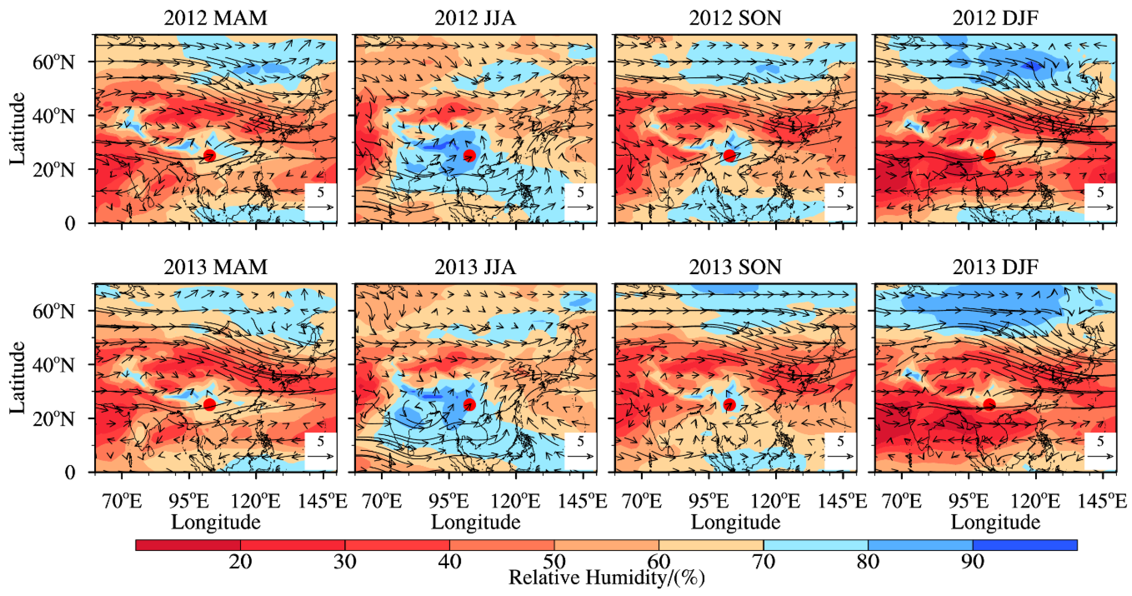
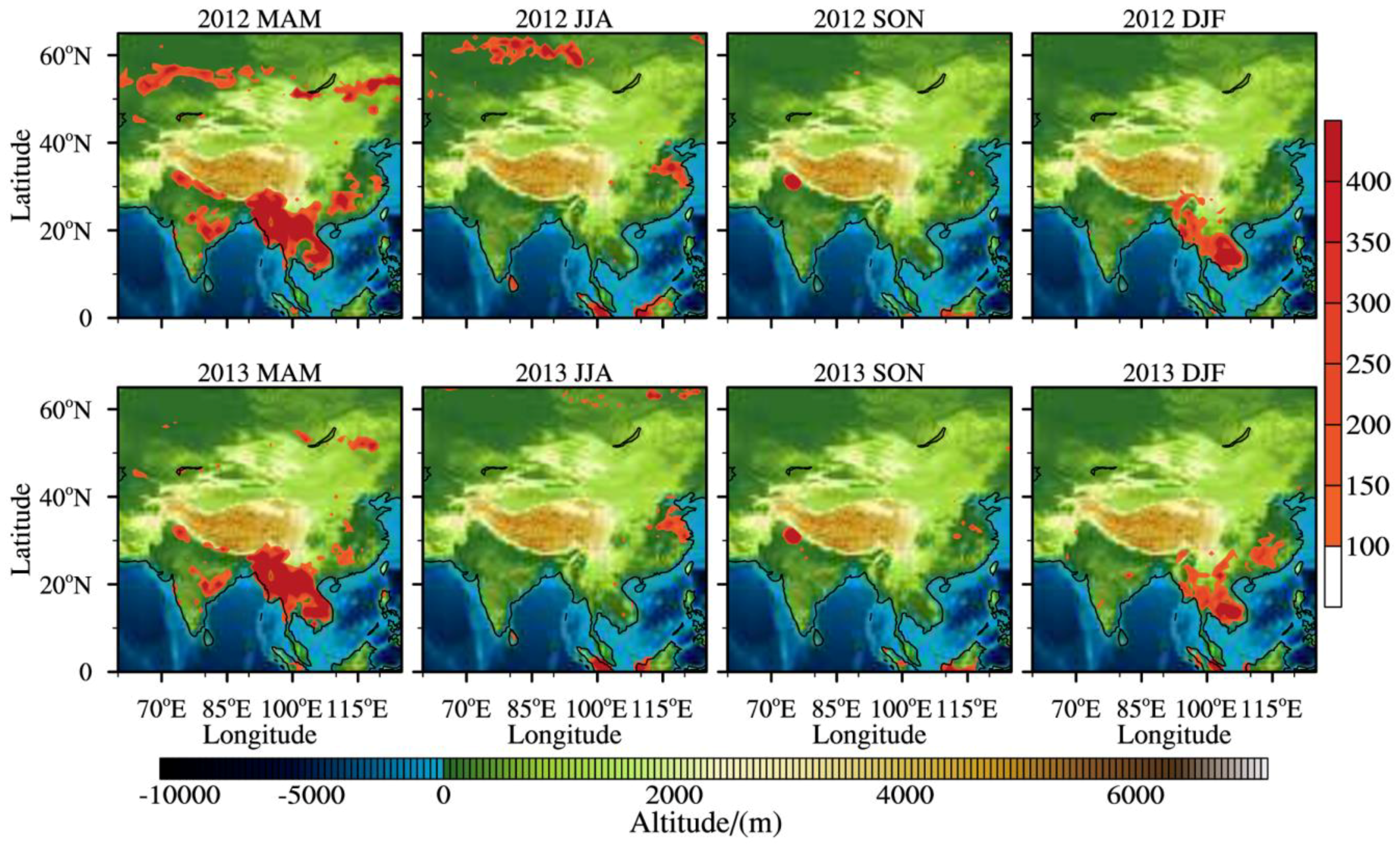
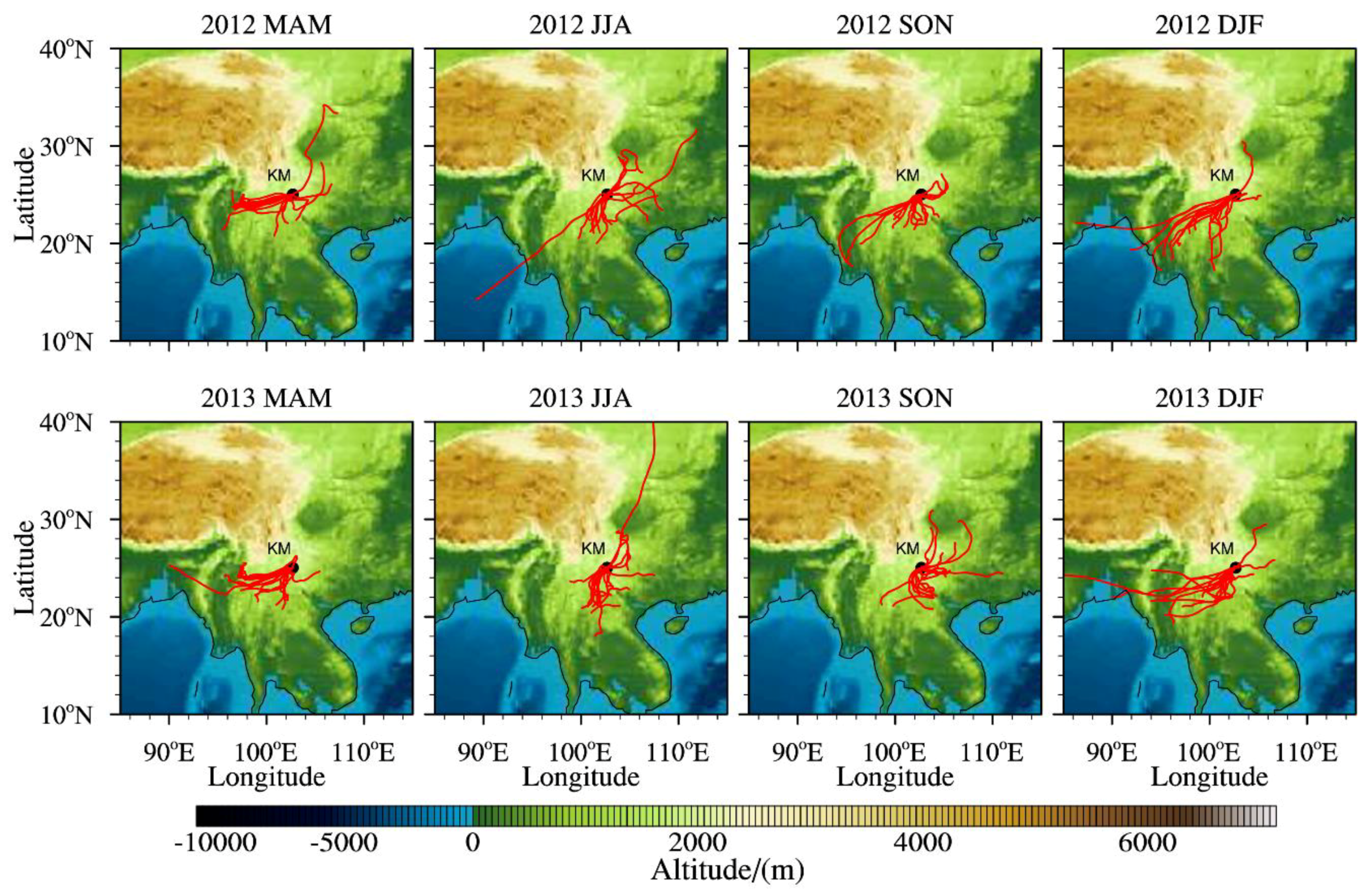
Kunming is located in the central part of the Yunnan–Kweichow Plateau and is affected by the East Asian monsoon and the South Asian monsoon. The annual sunshine is about 2200 h, and the ultraviolet radiation is strong. The monthly mean temperature is between 9.1 °C and 20.7 °C, and the monthly precipitation is between 11.3 mm and 204.0 mm. The precipitation in the rainy season from May to October accounts for 85% of the whole year and for more than 60% in summer. The southeast’s warm and humid airflow from the western Pacific and the southwest’s warm and humid airflow from the Indian Ocean meet over the Yunnan–Kweichow Plateau (which contains Yunnan), and a variety of aerosol species combine with water vapor to generate aerosol particles, which are transported over long distances (Southeast Asia–South Asia and the Iranian plateau to North Africa) [33,61], or the aerosol particles are hygroscopically grown. Under the conditions of a high temperature, high humidity, and strong ultraviolet radiation, chemical and photochemical reactions are favored to generate new aged aerosol particles. Therefore, due to the increase in the type and quantity of aerosol particles in summer (which makes the AOD reach its maximum), there is an increase in the volume concentration of the aerosol particles and the concentration of the coarse and fine particles. 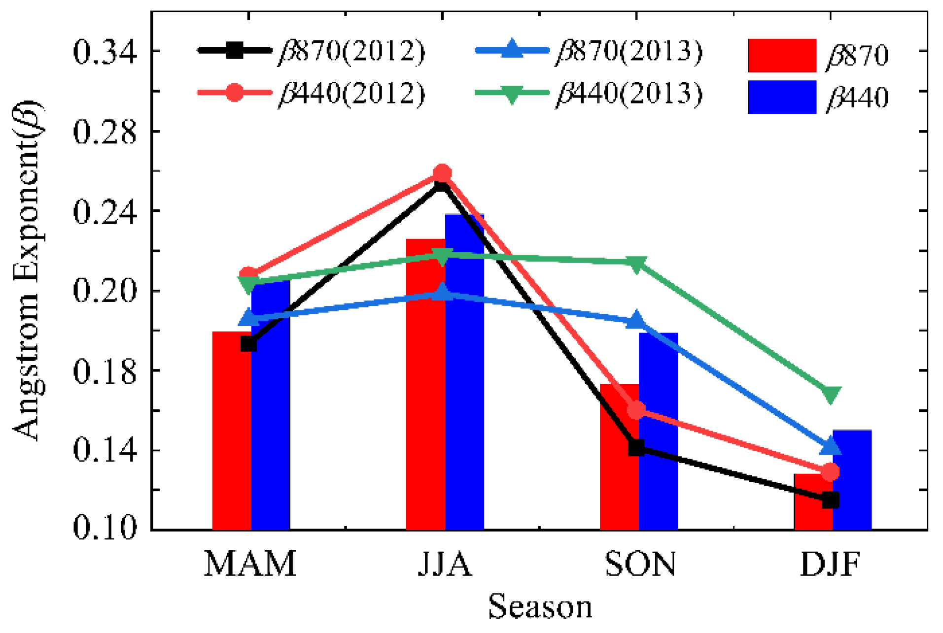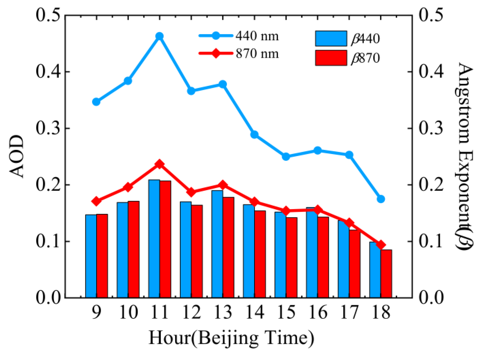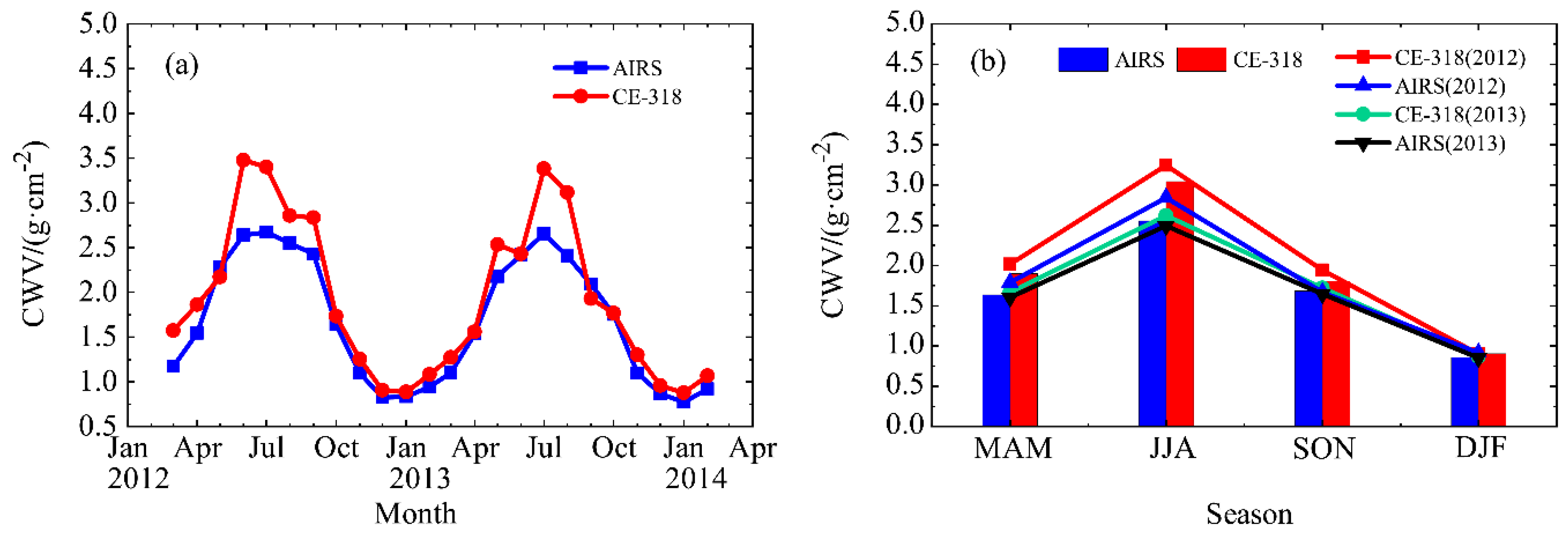Diversification of the particle size (the Angstrom Exponent (α) is higher than the annual mean value) affects the degree of the atmospheric turbidity (the β coefficient reaches the largest value). Because the physical, chemical, and optical properties (absorption and scattering cross section) of the aerosol changed greatly, the extinction effect was enhanced. Moreover, the increase of the water vapor (the CWV reaches the maximum value) enhances the extinction of the solar radiation absorption and scattering, which leads to the enhancement of the secondary or multiple scattering of the aerosol particles and promotes the variation of the aerosol properties.

Precipitation in the dry season from November to April of the following year accounts for only 15% of the whole year. There is little rain and plenty of sunshine in winter. It is mainly influenced by the west wind circulation and cold air from the higher latitude continent. The source and the physicochemical properties of the aerosol are different from those in the summer, which leads to the characteristic parameters of the AOD, CWV, and β coefficient change with the seasons and the AOD, CWV, and β coefficient reach the minimum values in winter.

In the spring, there are few clouds and little rain, the air is dry, the evapotranspiration is strong, the solar ultraviolet radiation is enhanced, and the diurnal range of the temperature is large. The temperature drops rapidly in the autumn, which is about 2 °C lower than that in the spring, the precipitation is reduced and less than 30% of summer (but more than that in spring and winter), and the air is dry. The values of the aerosol properties in spring and autumn are between those of summer and winter, but they are slightly different in the two seasons. Comparing the spring and autumn, the aerosol properties are higher (larger) to different degrees. The main reason is that the wind speed in the near–surface layer in spring is much larger than that in the autumn, so that the flying dust and floating dust generated by the exposed surface can enter the atmosphere, which makes the amount of aerosol particles increase slightly. The increase of the desert dust aerosol in spring makes the average AOD higher than that in autumn, and the particle radius changes obviously make the turbidity stronger. Due to the influence of the summer monsoon circulation, the CWV values in spring and autumn are quite different (there is no obvious difference and regularity). The wet season starts at the end of spring and ends in autumn, but the variations of the CWV in the two seasons are slightly different. A more specific difference analysis is needed to combine the characteristics of the actual monsoon circulation evolution with different years, characteristics of water vapor transport, and variation in meteorological factors.

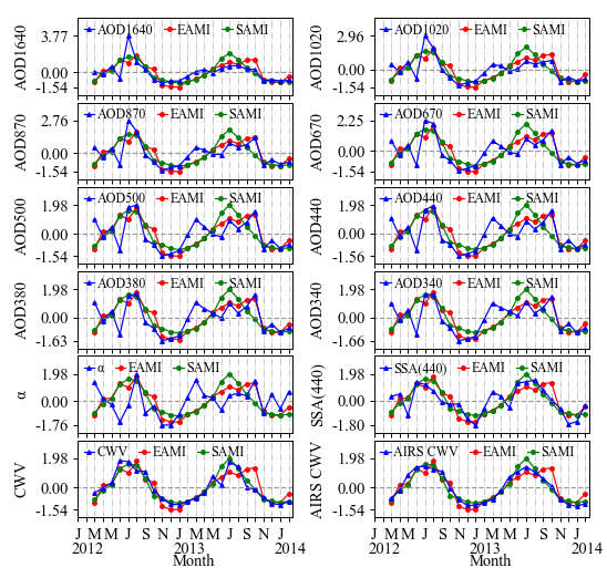
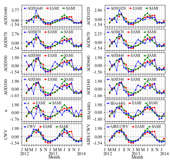
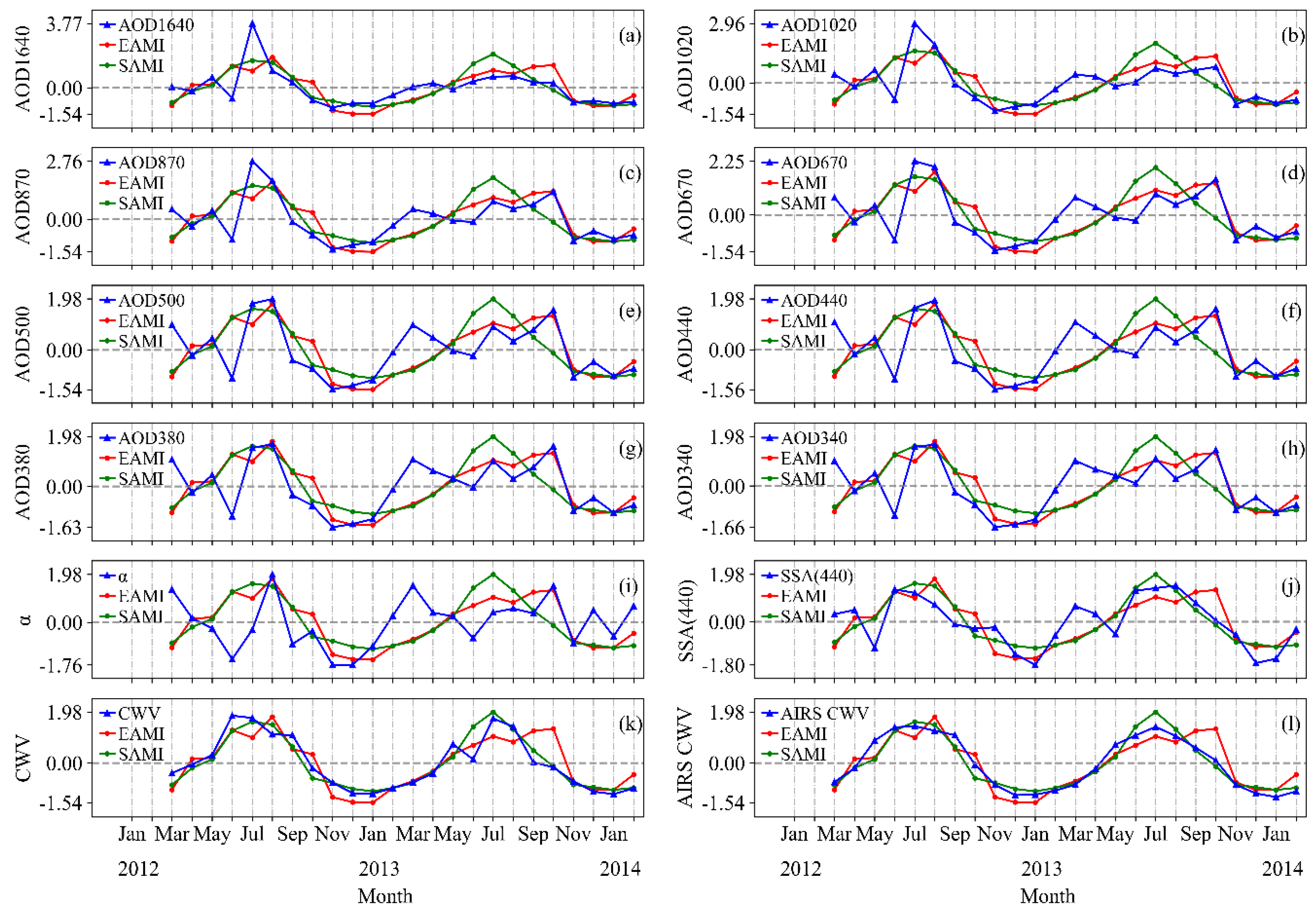
Figure 13 shows the characteristics of the seasonal variation and inter–annual activities of the EAMI and SAMI and aerosol properties normalized time series from March 2012 to February 2014. EAMI and SAMI are consistent with the variation in the aerosol properties, and the CWV and CWV (AIRS) are exactly the same as the seasonal variation of the monsoon index. The positive (negative) phase of the summer (winter) oscillation variation is significant, while those of spring and autumn are relatively weak, reflecting the difference in the aerosol type and source and the optical–radiation properties in different seasons. Except for the influence of other factors, it is mainly affected by the variation in the monsoon circulation activities (Figure A1 and Figure A3). The interannual variation difference of the monsoon circulation can also be reflected in the variation of the aerosol properties. The positive phase of the EAMI and SAMI variations in the summer of 2012 is much longer than that in 2013, resulting in the difference of the variation of the aerosol properties in the summer during those two years.

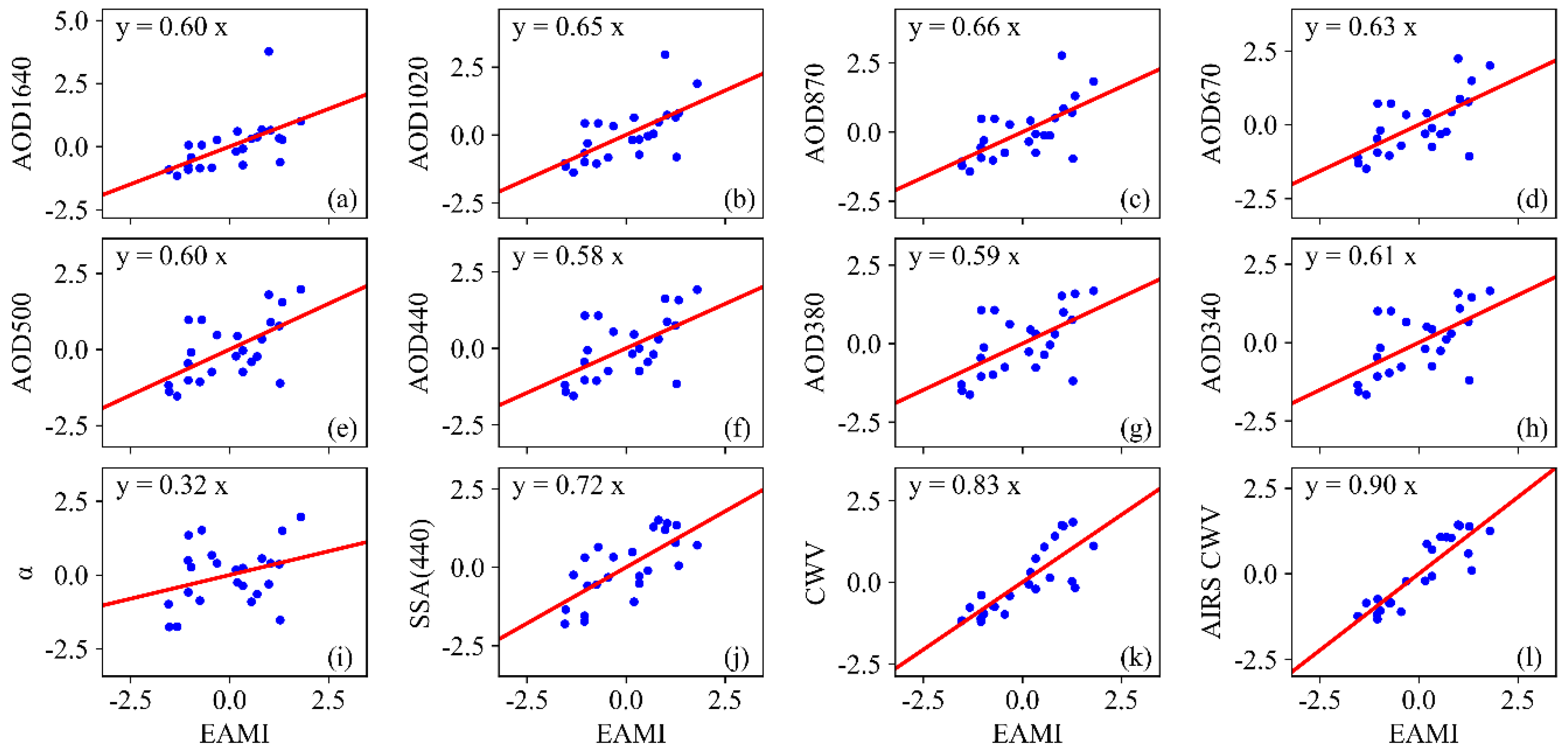
The linear fitting regression analysis of the aerosol properties and the monsoon index normalized sequence shows that y (the response of the aerosol properties to the monsoon circulation) = kx (the variation of the monsoon circulation). Only the influence of the monsoon circulation variation is considered here. The physical meaning of the slope k is the sensitivity of the aerosol properties to the monsoon circulation variation, while kx×% characterizes the relative influence rate of the monsoon circulation on the variation of the aerosol properties.

Figure 14 and Figure 15 show the correlation analysis of the normalized sequence between EAMI and SAMI and aerosol properties containing CWV (AIRS CWV). The CWV and CWV (AIRS) have the best linear relationship with the monsoon index. The relationship not only reflects the transport of the water vapor from the atmospheric circulation but also verifies the reliability of the aerosol properties retrieval. The linear relationship between the AOD at 8 bands, SSA at 440 nm, CWV (AIRS CWV), EAMI, and SAMI all pass the significance test of more than 99%, but the linear relationship between the Angstrom Exponent (α) and the monsoon index is relatively insignificant.

Table 2. Sensitivity k_E of the aerosol properties to the EAMI variation and the influence rate (%) of the East Asian monsoon circulation variation on the relative variation of the aerosol properties.

Year	Month	East Asian Monsoon Relative Impact Rate %
		Sensitivity kE of Aerosol Properties to EAMI variation
		0.60	0.65	0.66	0.63	0.60	0.58	0.59	0.61	0.32	0.72	0.83	0.90
		AOD1640	AOD1020	AOD870	AOD670	AOD500	AOD440	AOD380	AOD340	α	SSA	CWV	AIRS CWV
2012	Mar	−62.3	−68.1	−68.2	−65.7	−62.7	−60.6	−61.6	−63.1	−33.5	−74.5	−86.1	−93.3
	Apr	9.5	10.4	10.4	10.0	9.6	9.2	9.4	9.6	5.1	11.4	13.1	14.2
	May	11.8	12.9	12.9	12.4	11.9	11.5	11.7	11.9	6.4	14.1	16.3	17.7
	Jun	76.1	83.2	83.4	80.4	76.6	74.1	75.3	77.1	41.0	91.1	105.2	114.0
	Jul	59.0	64.6	64.7	62.3	59.4	57.5	58.5	59.8	31.8	70.7	81.6	88.5
	Aug	107.1	117.1	117.4	113.1	107.8	104.2	106.0	108.5	57.7	128.2	148.1	160.5
	Sep	32.6	35.7	35.8	34.5	32.9	31.8	32.3	33.1	17.6	39.1	45.1	48.9
	Oct	19.9	21.7	21.8	21.0	20.0	19.3	19.7	20.1	10.7	23.8	27.5	29.8
	Nov	−79.4	−86.9	−87.0	−83.9	−80.0	−77.3	−78.6	−80.5	−42.8	−95.1	−109.8	−119.0
	Dec	−91.2	−99.7	−99.9	−96.3	−91.8	−88.7	−90.3	−92.4	−49.1	−109.1	−126.1	−136.6
2013	Jan	−92.2	−100.8	−101.0	−97.3	−92.8	−89.7	−91.2	−93.4	−49.7	−110.3	−127.4	−138.1
	Feb	−58.4	−63.8	−64.0	−61.6	−58.7	−56.8	−57.8	−59.1	−31.4	−69.8	−80.7	−87.4
	Mar	−42.2	−46.1	−46.2	−44.5	−42.4	−41.0	−41.7	−42.7	−22.7	−50.5	−58.3	−63.2
	Apr	−19.1	−20.9	−20.9	−20.2	−19.2	−18.6	−18.9	−19.4	−10.3	−22.9	−26.4	−28.6
	May	20.0	21.8	21.9	21.1	20.1	19.4	19.8	20.2	10.8	23.9	27.6	29.9
	Jun	41.3	45.2	45.2	43.6	41.6	40.2	40.9	41.8	22.2	49.4	57.1	61.9
	Jul	61.8	67.6	67.8	65.3	62.2	60.2	61.2	62.7	33.3	74.0	85.5	92.6
	Aug	48.7	53.3	53.4	51.4	49.0	47.4	48.2	49.4	26.2	58.3	67.3	73.0
	Sep	74.6	81.5	81.7	78.7	75.0	72.5	73.8	75.5	40.2	89.2	103.1	111.7
	Oct	79.4	86.9	87.1	83.9	80.0	77.3	78.6	80.5	42.8	95.1	109.8	119.0
	Nov	−44.8	−49.0	−49.1	−47.3	−45.1	−43.6	−44.3	−45.4	−24.1	−53.6	−61.9	−67.1
	Dec	−62.9	−68.8	−68.9	−66.4	−63.3	−61.2	−62.3	−63.7	−33.9	−75.3	−86.9	−94.2
2014	Jan	−62.6	−68.5	−68.6	−66.1	−63.0	−60.9	−62.0	−63.4	−33.7	−74.9	−86.5	−93.8
	Feb	−26.9	−29.4	−29.5	−28.4	−27.1	−26.2	−26.6	−27.3	−14.5	−32.2	−37.2	−40.3

shows the sensitivity k_E of the aerosol properties to the EAMI variation and the influence rate (%) of the variation of the East Asian monsoon circulation on the relative variation of the aerosol properties.

During the dry season, from November to March (or April) of the following year, the aerosol characteristic parameter value decreases with the weakening of the East Asian monsoon circulation (negative phase) and reaches the minimum value in January. During the spring/summer transition from March (or April) to May, the positive phase of the East Asian monsoon circulation variation gradually increases. At this time, the variation of the aerosol characteristic parameter value under the influence of the monsoon circulation starts to change from decreasing to increasing. During the rainy season from May to October, the values of the aerosol properties increase rapidly in the period of the East Asian monsoon circulation enhancement (positive phase). It should be noted that the aerosol properties reached a maximum value in August 2012. However, the maximum value not only was delayed by two months but was relatively small. It shows that the interannual activity of the East Asian monsoon circulation is significantly different. The negative phase of the East Asian monsoon circulation variation gradually increases during the autumn–winter transition from October to November. At this time, the variation of the aerosol characteristic parameter value begins to change from increasing to decreasing due to the variation of the monsoon circulation. The transformation of the positive and negative (negative and positive) phases of the monsoon circulation affects the seasonal variation characteristics of the aerosol properties. However, the activity intensity of the monsoon circulation in different years and the difference in the transition period have different effects on different aerosol properties. Except for the CWV (AIRS CWV), the effect of the SSA on the 440 nm band is the most significant, and the effect on the AOD at different wavelengths is more consistent.

Table 3. Sensitivity k_S of the aerosol properties to the SAMI variation and the influence rate (%) of the South Asian monsoon circulation on the relative variation of the aerosol properties.

Year	Month	South Asian Monsoon Relative Impact Rate %
		Sensitivity kS of Aerosol Properties to EAMI Variation
		0.69	0.65	0.62	0.55	0.51	0.48	0.49	0.52	0.10	0.77	0.93	0.95
		AOD1640	AOD1020	AOD870	AOD670	AOD500	AOD440	AOD380	AOD340	α	SSA	CWV	AIRS CWV
2012	Mar	−58.9	−55.4	−52.4	−47.2	−43.0	−40.7	−42.0	−44.6	−8.8	−65.9	−79.0	−81.1
	Apr	−13.7	−12.9	−12.2	−10.9	−10.0	−9.4	−9.7	−10.3	−2.0	−15.3	−18.3	−18.8
	May	9.9	9.3	8.8	7.9	7.2	6.8	7.0	7.5	1.5	11.0	13.2	13.6
	Jun	86.5	81.4	77.0	69.3	63.2	59.7	61.6	65.4	13.0	96.8	116.1	119.2
	Jul	111.1	104.6	98.9	89.0	81.1	76.7	79.1	84.1	16.6	124.3	149.1	153.1
	Aug	103.5	97.4	92.0	82.9	75.5	71.4	73.7	78.3	15.5	115.7	138.8	142.5
	Sep	43.7	41.1	38.9	35.0	31.9	30.2	31.1	33.0	6.5	48.9	58.6	60.2
	Oct	−41.0	−38.6	−36.5	−32.9	−30.0	−28.3	−29.2	−31.0	−6.1	−45.9	−55.1	−56.5
	Nov	−53.6	−50.4	−47.6	−42.9	−39.1	−37.0	−38.1	−40.5	−8.0	−59.9	−71.8	−73.8
	Dec	−69.8	−65.7	−62.1	−55.9	−51.0	−48.2	−49.7	−52.8	−10.5	−78.1	−93.7	−96.2
2013	Jan	−76.4	−71.9	−67.9	−61.2	−55.8	−52.7	−54.4	−57.8	−11.4	−85.4	−102.5	−105.2
	Feb	−67.3	−63.4	−59.9	−53.9	−49.2	−46.5	−48.0	−50.9	−10.1	−75.3	−90.3	−92.8
	Mar	−54.5	−51.3	−48.5	−43.6	−39.8	−37.6	−38.8	−41.2	−8.2	−60.9	−73.1	−75.0
	Apr	−23.2	−21.8	−20.6	−18.6	−16.9	−16.0	−16.5	−17.5	−3.5	−25.9	−31.1	−31.9
	May	16.8	15.8	15.0	13.5	12.3	11.6	12.0	12.7	2.5	18.8	22.6	23.2
	Jun	98.0	92.2	87.1	78.5	71.5	67.6	69.8	74.1	14.7	109.6	131.4	134.9
	Jul	137.3	129.2	122.1	109.9	100.2	94.8	97.8	103.8	20.6	153.6	184.2	189.1
	Aug	90.9	85.6	80.9	72.8	66.4	62.8	64.7	68.8	13.6	101.7	122.0	125.2
	Sep	33.5	31.6	29.8	26.9	24.5	23.2	23.9	25.4	5.0	37.5	45.0	46.2
	Oct	−9.3	−8.7	−8.2	−7.4	−6.8	−6.4	−6.6	−7.0	−1.4	−10.4	−12.4	−12.8
	Nov	−58.7	−55.2	−52.2	−47.0	−42.8	−40.5	−41.8	−44.4	−8.8	−65.6	−78.7	−80.8
	Dec	−65.3	−61.4	−58.1	−52.3	−47.6	−45.1	−46.5	−49.4	−9.8	−73.0	−87.6	−89.9
2014	Jan	−72.7	−68.4	−64.6	−58.2	−53.0	−50.2	−51.7	−55.0	−10.9	−81.3	−97.5	−100.1
	Feb	−66.9	−63.0	−59.5	−53.6	−48.9	−46.2	−47.7	−50.6	−10.0	−74.9	−89.8	−92.2

shows the sensitivity k_S of the aerosol properties to the SAMI variation and influence rate (%) of the South Asian monsoon circulation on the relative variation of the aerosol properties. Compared with the East Asian monsoon circulation, the South Asian monsoon circulation weakens 1 month earlier. From October to April of the following year, the South Asian monsoon circulation weakens, and the aerosol characteristic parameter values decrease accordingly, also reaching a minimum value in January. During the transition period from April to May, the monsoon circulation has little effect on the variation of the aerosol properties due to the aerosol characteristic parameter values’ change from decreasing to increasing.

From May to September, the South Asian monsoon circulation increases, and the aerosol characteristic parameter values continued to increase, reaching a maximum value in August. During the transition period from September to October, the South Asian monsoon circulation begins to weaken, which changes the aerosol characteristic parameter value from increasing to decreasing and the impact of the variation of the monsoon circulation on the aerosol characteristic parameter values is also small.

By combining Table 2 and Table 3, it is clear that the effects of the East Asian monsoon and the South Asian monsoon on the variation in aerosol properties are similar. Although there is a seasonal difference, the synergy between the East Asian monsoon and the South Asian monsoon is obvious, and the variation in the aerosol properties is consistent with their seasonal variations. The sensitivity of the CWV and CWV (AIRS) to the EAMI and SAMI variations is 0.83–0.90 and 0.93–0.95, respectively. The CWV (AIRS CWV) is more significantly affected by the South Asian monsoon than the East Asian monsoon, which indicates the contribution of the water vapor from the atmospheric circulation. The sensitivity of the SSA in the 440 nm band to the EAMI and SAMI is 0.72 and 0.77, while the sensitivity of the AOD for different λ to the EAMI and SAMI ranges from 0.58 to 0.66 (mean value is 0.62) and 0.48 to 0.69 (mean value is 0.56), which indicates that the extinction of the aerosol particles is deeply affected by the variation of the monsoon circulation activity. It is also noted that the sensitivity of the AOD to the EAMI is greater than that of the SAMI, and the influence of the inter–monthly variation of the EAMI on the aerosol properties is more drastic than that of the SAMI. This may be due to the complexity of the East Asian monsoon and the South Asian monsoon in the process of converging over the Yunnan–Kweichow Plateau, which needs to be studied in detail.

In summary, aerosol properties that vary with the seasons are affected and controlled by the variation in the monsoon circulation activity. For example, the AOD is closely related to the seasonal variation of the CWV. The increase of the water vapor content can affect the variation of the aerosol particle size and quantity, and the physical and chemical reactions of aerosol particles, which promotes the increase of the AOD caused by the extinction of the aerosol. In 2012 and 2013, the variation difference of the monsoon circulation can affect and control the difference in the aerosol sources and types, and the variation in the intensity of the seasonal and interannual activity may also change the number of aerosol particles and the formation difference of the aged aerosol. However, since only two years of data were used, it is necessary to verify whether it is credible through the evaluation of longer–term data. In addition, it should be noted that except for the influence of the monsoon circulation, there is an impact from the increased local emissions of fugitive dust on the aerosol properties. For example, the differences between the interannual and monthly variation in the aerosol properties in Kunming in 2012 and 2013 are not only related to the interannual differences in monsoon circulation but also related to the increase in the local emissions.

7. Conclusions

The relationship between the influence of the East Asian and South Asian monsoon index on the seasonal variation of the aerosol properties is discussed below based on the retrieval of the aerosol optical and radiation properties from the observational data of the CE–318 sunphotometer at the Kunming atmospheric ozone monitoring station. The conclusions are as follows.

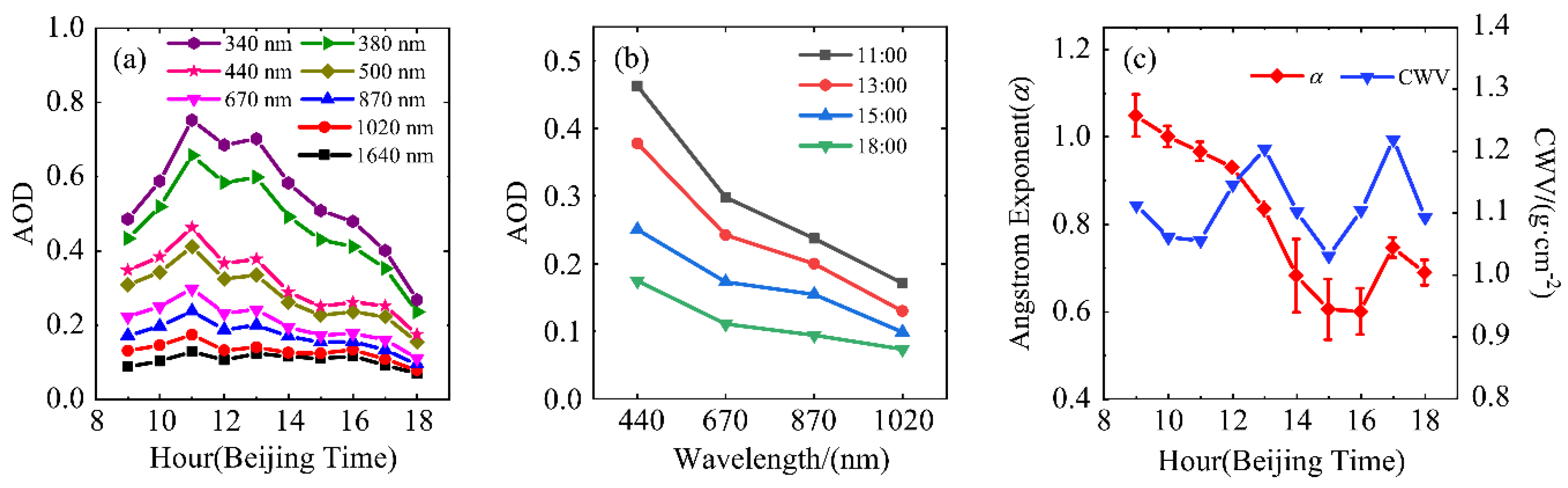
The AOD decreases with the increase of λ and is consistent with the typical Mie scattering properties. The seasonal variation of the AOD, Angstrom turbidity coefficient β, and CWV is unimodal, the summer (winter) is the largest (smallest), and the spring is greater than the autumn. The CWV values in spring and autumn showed no significant difference, and the seasonal variation of the Angstrom Exponent (α) was not obvious. The turbidity in the atmosphere was relatively low. This indicates that the aerosol properties of the low–latitude plateaus in southwestern China are different from those in other parts of China. Although they are affected by anthropogenic emissions from the Southeast Asia–South Asia region and biomass burning aerosols, the correlation between the intensity of the seasonal activities of the monsoon circulation and the local anthropogenic emissions and meteorological factors will affect the aerosol properties, so further in–depth simulation studies are needed.

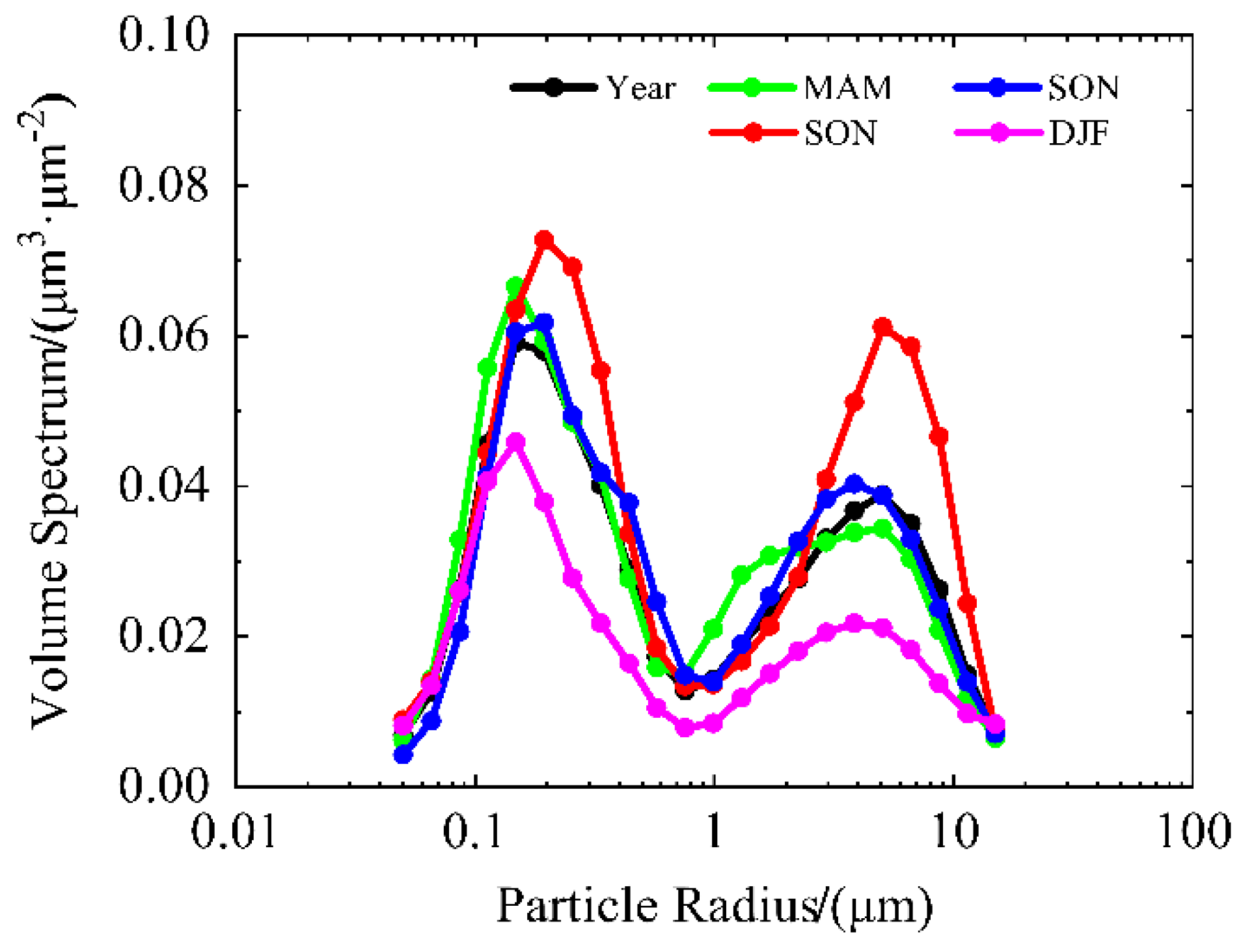
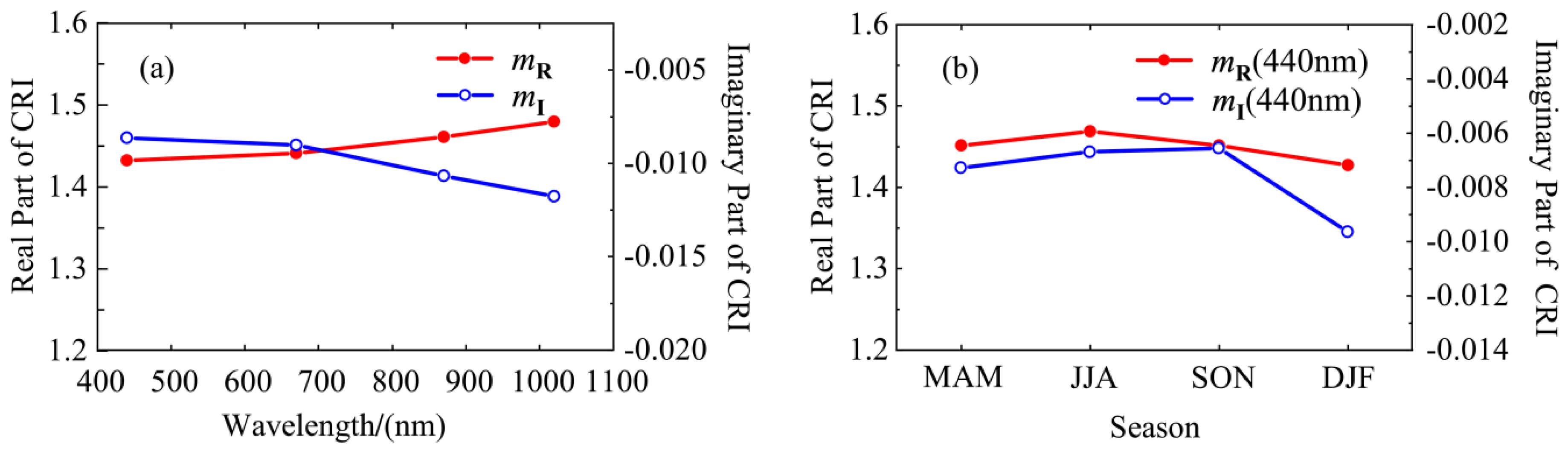
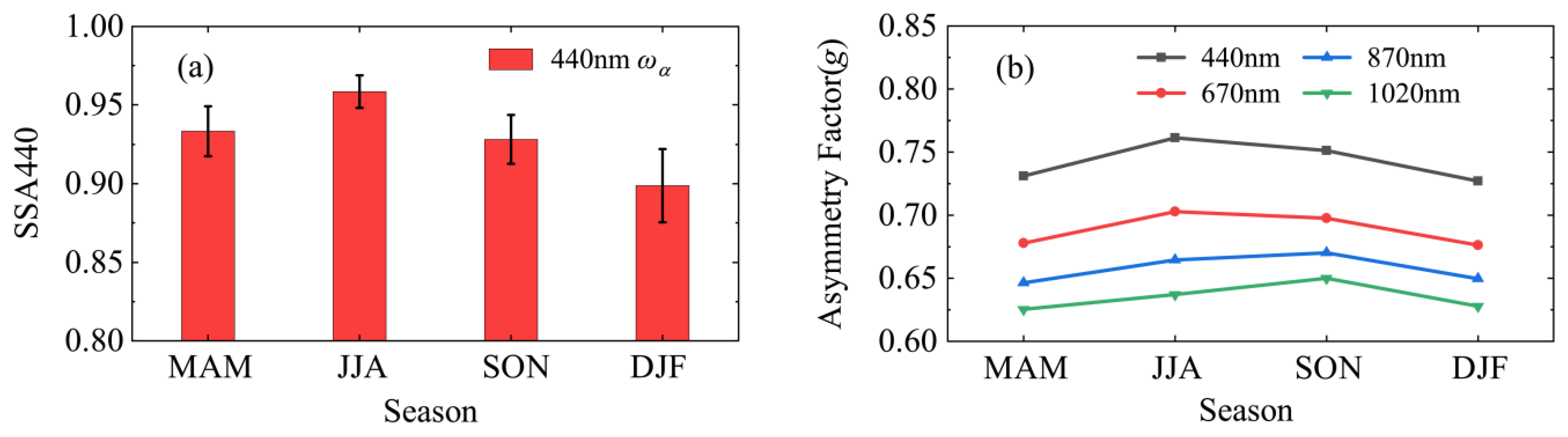
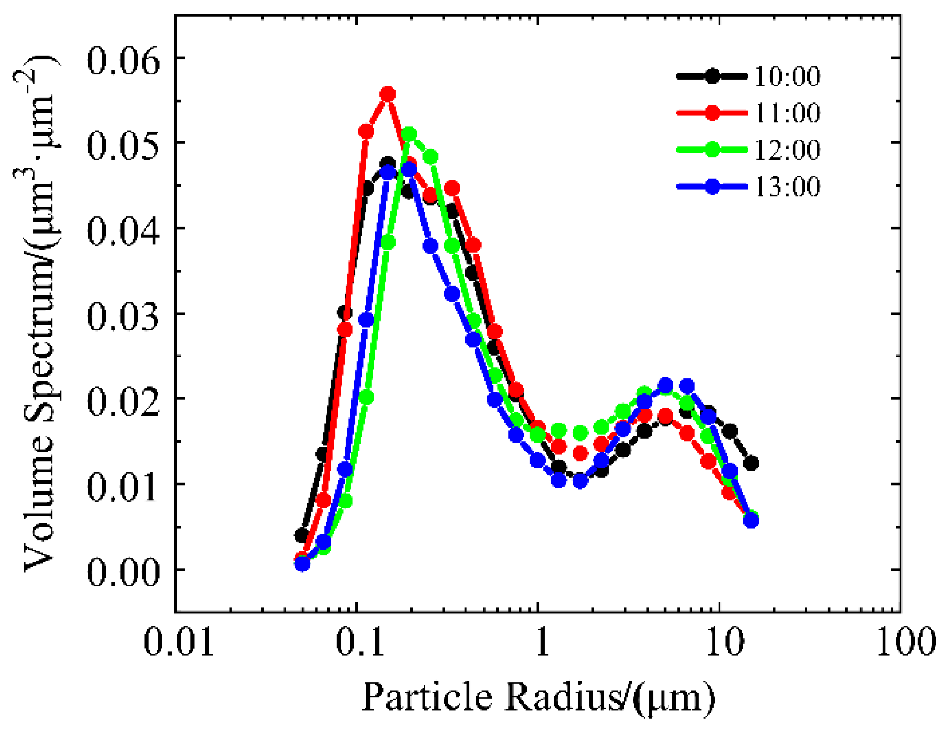
The seasonal and annual variations of the aerosol particle size distributions are bimodal. The complex refractive index and single scattering albedo showed that the summer aerosol particles had a stronger scattering power and a relatively weak absorption power; in winter, they exhibited the opposite. In summer, the water vapor content was high, and after the hygroscopic aerosol particles absorbed water, the particle size and volume increased, resulting in enhanced scattering. In order to explain the enhancement of the aerosol absorption capacity in winter, the retrieval result for the FI needs to be further discussed.

The variation of the aerosol properties with the season was significantly affected by the monsoon circulation activity, and the synergistic effect of the East Asian monsoon and South Asian monsoon made the variation of the aerosol properties have the same seasonal oscillation characteristics as that of the monsoon. In the transition period of the season (especially during the transition periods of the dry and wet seasons in Kunming), the monsoon circulation had little effect on the variation of the aerosol properties. The AOD was closely related to the seasonal variation of the CWV. The increase or decrease of the water vapor content did affect the variation of the aerosol particle size and quantity, thus affecting the physical and chemical reactions of the aerosol particles. Furthermore, the extinction of the aerosol was promoted to cause an increase in the AOD. Only in 2012 and 2013 did the variation difference of the monsoon circulation affect the source and type of aerosol. The variation in the intensity of the seasonal and interannual activity may have also changed the number of aerosol particles and the formation difference of the aged aerosol. It should also be noted that, in addition to the influence of the monsoon circulation, there was an impact from the increased local emissions of fugitive dust on the aerosol properties.

8. Discussion

This study only dealt with the retrieval and discussion of the aerosol properties in Kunming. Follow–up work needs to compare the aerosol properties of the retrieval between the satellite data and CE–318 observation data. We need to simulate the seasonal variation for the monsoon circulation activity variation and aerosol type and source in greater depth, as well as the direct radiative forcing effects of aerosols. This study investigated a limited time span of the observational data from the Kunming atmospheric ozone monitoring station, so the rule of seasonal change needs data from a longer period of time, and the long–term evolution trend of the interannual and interdecadal variations needs further research. Furthermore, a more in–depth statistical analysis of the relationship between the aerosol properties and meteorological elements is needed.

References

1. Holben, B.; Tanré, D.; Smirnov, A.; Eck, T.; Slutsker, I.; Abuhassan, N.; Newcomb, W.; Schafer, J.; Chatenet, B.; Lavenu, F.; et al. An emerging ground–based aerosol climatology: Aerosol optical depth from AERONET. J. Geophys. Res. Atmos. 2001, 106, 12067–12097. [Google Scholar] [CrossRef]
2. Di, H.G.; Wang, Q.Y.; Hua, H.B.; Li, S.W.; Yan, Q.; Liu, J.J.; Song, Y.H.; Hua, D.X. Aerosol Microphysical Particle Parameter Inversion and Error Analysis Based on Remote Sensing Data. Remote Sens. 2018, 10, 1753. [Google Scholar] [CrossRef] [Green Version]
3. Stachlewska, I.S.; Samson, M.; Zawadzka, O.; Harenda, K.M.; Janicka, L.; Poczta, P.; Janicka, L.; Poczta, P.; Szczepanik, D.; Heese, B.; et al. Modification of Local Urban Aerosol Properties by Long–Range Transport of Biomass Burning Aerosol. Remote Sens. 2018, 10, 412. [Google Scholar] [CrossRef] [Green Version]
4. Zhang, Y.; Li, Z.Q.; Liu, Z.H.; Zhang, J.; Qie, L.L.; Xie, Y.S.; Hou, W.Z.; Wang, Y.Q.; Ye, Z.X. Retrieval of the Fine–Mode Aerosol Optical Depth over East China Using a Grouped Residual Error Sorting (GRES) Method from Multi–Angle and Polarized Satellite Data. Remote Sens. 2018, 10, 1838. [Google Scholar] [CrossRef] [Green Version]
5. Estellés, V.; Campanelli, M.; Expósito, F.; Utrillas, M.; Martínez–Lozano, J. Aerosol Radiative Forcing in the European Skynet Radiometers Network; European Geosciences Union: Munich, Germany, 2012; Available online: https://meetingorganizer.copernicus.org/EGU2012/EGU2012-10204.pdf (accessed on 30 December 2012).
6. Su, X.L.; Cao, J.J.; Li, Z.Q.; Li, K.T.; Xu, H.; Liu, S.X.; Fan, X.H. Multi–Year Analyses of Columnar Aerosol Opticaland Microphysical Properties in Xi’an, a Megacity inNorthwestern China. Remote Sens. 2018, 10, 1169. [Google Scholar] [CrossRef] [Green Version]
7. Li, Z.B.; Roy, D.P.; Zhang, H.K.; Vermote, E.F.; Huang, H.Y. Vermote and Haiyan Huang, Evaluation of Landsat–8 and Sentinel–2A Aerosol Optical Depth Retrievals across Chinese Cities and Implications for Medium Spatial Resolution Urban Aerosol Monitoring. Remote Sens. 2019, 11, 122. [Google Scholar] [CrossRef] [Green Version]
8. Zhang, L.; Li, J. Variability of Major Aerosol Types in China Classified Using AERONET Measurements. Remote Sens. 2019, 11, 2334. [Google Scholar] [CrossRef] [Green Version]
9. Tao, M.; Chen, L.; Wang, Z.; Tao, J.; Che, H.; Wang, X.; Wang, Y. Comparison and evaluation of the MODIS Collection 6 aerosol data in China. J. Geophys. Res. Atmos. 2015, 120, 6992–7005. [Google Scholar] [CrossRef]
10. Che, H.; Xia, X.; Zhu, J.; Li, Z.; Dubovik, O.; Holben, B.; Goloub, P.; Chen, H.; Estelles, V.; Cuevas-Agulló, E. Column aerosol optical properties and aerosol radiative forcing during a serious haze–fog month over North China Plain in 2013 based on ground–based sunphotometer measurements. Atmos. Chem. Phys. 2014, 14, 2125–2138. [Google Scholar] [CrossRef] [Green Version]
11. Qin, W.M.; Liu, Y.; Wang, L.C.; Lin, A.W.; Xia, X.G.; Che, H.Z.; Bilal, M.; Zhang, M. Characteristic and Driving Factors of Aerosol OpticalDepth over Mainland China during 1980–2017. Remote Sens. 2018, 10, 1064. [Google Scholar] [CrossRef] [Green Version]
12. McPhetres, A.; Aggarwal, S. An Evaluation of MODIS–Retrieved Aerosol Optical Depth over AERONET Sites in Alaska. Remote Sens. 2018, 10, 1384. [Google Scholar] [CrossRef] [Green Version]
13. Lopes, F.J.S.; Silva, J.J.; Marrero, J.C.A.; Taha, G.; Landulfo, E. Synergetic Aerosol Layer Observation After the 2015 Calbuco Volcanic Eruption Event. Remote Sens. 2019, 11, 195. [Google Scholar] [CrossRef] [Green Version]
14. Holben, B.; Eck, T.; Slutsker, I.; Tanré, D.; Buis, J.; Setzer, A.; Vermote, E.; Reagan, J.; Kaufman, Y.; Nakajima, T.; et al. AERONET—A Federated Instrument Network and Data Archive for Aerosol Characterization. Remote Sens. Environ. 1998, 66, 1–16. [Google Scholar] [CrossRef]
15. Uchiyama, A.; Yamazaki, A.; Togawa, H.; Asano, J. Characteristics of Aeolian dust observed by SKY–Radiometer in the Intensive Observation Period 1 (IOP1). J. Meteorol. Soc. Jpn. 2005, 83, 291–305. [Google Scholar] [CrossRef] [Green Version]
16. Takamura, T.; Takenaka, H.; Cui, Y.; Nakajima, T.; Higurashi, A.; Fukuda, S.; Kikuchi, N.; Nakajima, T.; Sano, I.; Pinker, R. Aerosol and Cloud Validation System Based on SKYNET Observations: Estimation of Shortwave Radiation Budget Using ADEOS–II/GLI Data. J. Remote Sens. Soc. Jpn. 2009, 29, 40–53. [Google Scholar]
17. Wehrli, C. GAWPFR: A Network of Aerosol Optical Depth Observations with Precision Filter Radiometers. WMO/GAW Experts Workshop on a Global Surface–Based Network for Long Term Observations of Column Aerosol Optical Properties. 2005. Available online: https://library.wmo.int/index.php?lvl=notice_display&id=11094#.XeYm625uKM9 (accessed on 12 December 2006).
18. Che, H.; Zhang, X.; Chen, H.; Damiri, B.; Goloub, P.; Li, Z.; Zhang, X.; Wei, Y.; Zhou, H.; Dong, F.; et al. Instrument calibration and aerosol optical depth validation of the China Aerosol Remote Sensing Network. J. Geophys. Res. Atmos. 2009, 114, D03206. [Google Scholar] [CrossRef]
19. Xin, J.; Wang, Y.; Li, Z.; Wang, P.; Wang, S.; Wen, T.; Sun, Y. Introduction and Calibration of the Chinese Sun Hazemeter Network. Chin. J. Environ. Sci. 2006, 27, 1697–1702. [Google Scholar]
20. Xin, J.; Wang, Y.; Pan, Y.; Ji, D.; Liu, Z.; Wen, T.; Wang, Y.; Li, X.; Sun, Y.; Sun, J.; et al. The Campaign on Atmospheric Aerosol Research Network of China: CARE–China. Bull. Am. Meteorol. Soc. 2015, 96, 1137–1155. [Google Scholar] [CrossRef]
21. Mangold, A.; Backer, H.D.; Paepe, B.D.; Dewitte, S.; Chiapello, I.; Derimian, Y.; Kacenelenbogen, M.; Léon, J.-F.; Huneeus, N.; Schulz, M.; et al. Aerosol analysis and forecast in the European Centre for Medium–Range Weather Forecasts Integrated Forecast System: 3. Evaluation by means of case studies. J. Geophys. Res. 2011, 116, D03302. [Google Scholar]
22. Zhang, M.; Wang, L.C.; Bilal, M.; Gong, W.; Zhang, Z.Y.; Guo, G.M. The Characteristics of the Aerosol Optical Depth within the Lowest Aerosol Layer over the TibetanPlateau from 2007 to 2014. Remote Sens. 2018, 10, 696. [Google Scholar] [CrossRef] [Green Version]
23. Kim, M.; Kim, J.; Torres, O.; Ahn, C.; Kim, W.; Jeong, U.; Go, S.J.; Liu, X.; Moon, K.J.; Kim, D.-R. Optimal Estimation–Based Algorithm to RetrieveAerosol Optical Properties for GEMS Measurementsover Asia. Remote Sens. 2018, 10, 162. [Google Scholar] [CrossRef] [Green Version]
24. Zhang, L.; Zhang, M.; Yao, Y.B. Multi–Time Scale Analysis ofRegional AerosolOptical Depth Changes in National–Level UrbanAgglomerations in China Using Modis Collection6.1 Datasets from 2001 to 2017. Remote Sens. 2019, 11, 201. [Google Scholar] [CrossRef] [Green Version]
25. Lin, C.A.; Chen, Y.C.; Liu, C.Y.; Chen, W.T.; Seinfeld, J.H.; Chou, C.C.-K. Satellite–Derived Correlation of SO2, NO2, andAerosol Optical Depth with Meteorological Conditions over East Asia from 2005 to 2015. Remote Sens. 2019, 11, 1738. [Google Scholar] [CrossRef] [Green Version]
26. Dubovik, O.; King, M. A flexible inversion algorithm for retrieval of aerosol optical properties from Sun and sky radiance measurements. J. Geophys. Res. Atmos. 2000, 105, 20673–20696. [Google Scholar] [CrossRef] [Green Version]
27. Olmo, F.; Quirantes, A.; Alcántara, A.; Lyamani, H.; Alados-Arboledas, L. Preliminary results of a non–spherical aerosol method for the retrieval of the atmospheric aerosol optical properties. J. Quant. Spectrosc. Radiat. Transf. 2006, 100, 305–314. [Google Scholar] [CrossRef]
28. Estellés, V.; Smyth, T.; Campanelli, M.; Utrillas, M. Development of an open source package for the processing of Sun–sky photometric data in the European Skyrad Users network (ESR). In Proceedings of the EGU General Assembly, Vienna, Austria, 19–24 April 2009; Volume 11, pp. EGU2009–EGU10952. Available online: https://meetingorganizer.copernicus.org/EGU2009/EGU2009-10952.pdf (accessed on 30 December 2009).
29. He, Q.; Yang, Y.; Geng, F.; Zhou, G.; Liu, D.; Wang, W. Algorithm comparison of aerosol parameter retrieval from sunphotometer measurements. Acta Meteorol. Sin. 2010, 68, 428–438. [Google Scholar]
30. Nakajima, T.; Tonna, G.; Rao, R.; Boi, P.; Kaufman, Y.; Holben, B. Use of sky brightness measurements from ground for remote sensing of particulate polydispersions. Appl. Opt. 1996, 35, 2672–2686. [Google Scholar] [CrossRef]
31. Huang, H.; Yi, W.; Qiao, Y. A method for retrieving aerosol optical properties based on Sun photometer. J. Atmos. Environ. Opt. 2012, 7, 175–180. [Google Scholar]
32. Estellés, V.; Campanelli, M.; Utrillas, M.; Expόsito, F.; Martínez–Lozano, J. Comparison of AERONET and SKYRAD4.2 inversion products retrieved from a Cimel CE318 sunphotometer. Atmos. Meas. Tech. 2012, 5, 569–579. [Google Scholar] [CrossRef] [Green Version]
33. Streets, D.; Yarber, K.; Woo, J.; Carmichael, G. Biomass burning in Asia: Annual and seasonal estimates and atmospheric emissions. Glob. Biogeochem. Cycles 2003, 17. [Google Scholar] [CrossRef] [Green Version]
34. Sahu, L.; Saxena, P. High time and mass resolved PTR–TOF–MS measurements of VOCs at an urban site of India during winter: Role of anthropogenic, biomass burning, biogenic and photochemical sources. Atmos. Res. 2015, 64, 84–94. [Google Scholar] [CrossRef]
35. Gui, K.; Che, H.; Chen, Q.; Zeng, Z.; Zheng, Y.; Long, Q.; Sun, T.; Liu, X.; Wang, Y.; Liao, T.; et al. Water vapor variation and the effect of aerosols in China. Atmos. Environ. 2017, 165, 322–335. [Google Scholar] [CrossRef]
36. Zhu, J.; Che, H.; Xia, X.; Yu, X.; Wang, J. Analysis of water vapor effects on aerosol properties and direct radiative forcing in China. Sci. Total Environ. 2019, 650, 257–266. [Google Scholar] [CrossRef] [PubMed]
37. Tao, R.; Che, H.; Chen, Q.; Wang, Y.; Sun, J.; Zhang, X.; Lu, S.; Guo, J.; Wang, H.; Zhang, X. Development of an integrating sphere calibration method for Cimel sunphotometers in China aerosol remote sensing network. Particuology 2014, 13, 88–99. [Google Scholar] [CrossRef]
38. Yang, Z.; Zhang, X.; Che, H.; Zhang, X.; Hu, X.; Zhang, L. An Introductory Study on the Calibration of CE318 Sunphotometer. J. Appl. Meteorol. Sci. 2008, 19, 297–306. [Google Scholar]
39. Giglio, L. MODIS Collection 5 Active Fire Product User’s Guide Version 2.5. 2013. Available online: http://modis-fire.umd.edu/files/MODIS_Fire_Users_Guide_2.5.pdf (accessed on 30 December 2013).
40. Liu, J.; Niu, S.J.; Zheng, Y.F. Optical Depth Characteristics of Yinchuan Atmospheric Aerosols Based on the CE–318 Sun Tracking Spectrophotometer Data. J. Nanjing Inst. Meteorol. 2004, 27, 615–622. [Google Scholar]
41. Zhu, X.S.; Zhou, J. Determination of Clear–Sky Columnar Water Vapor Using Solar Radiometer. Sci. Atmos. Sin. 1998, 22, 40–46. [Google Scholar]
42. Schmechtig, C.; Santer, R.P.; Roger, J.C.; Meygret, A. Automatic ground–based station for vicarious calibration. Proc. SPIE-Int. Soc. Opt. Eng. 1997, 3221, 309–317. [Google Scholar]
43. Junge, C. The Size Distribution and Aging of Natural Aerosols as Determined from Electrical and Optical Data on the Atmosphere. J. Atmos. Sci. 1955, 12, 13–25. [Google Scholar] [CrossRef] [Green Version]
44. Ångström, A. On the atmospheric transmission of Sun radiation and on dust in the air. Geografiska Annaler 1929, 11, 156–166. [Google Scholar]
45. O’Neill, N.; Dubovik, O.; Eck, T. Modified Ångström exponent for the characterization of submicrometer aerosols. Appl. Opt. 2001, 40, 2368–2375. [Google Scholar] [CrossRef]
46. Tanré, D.; Kaufman, Y.J.; Holben, B.N.; Chatenet, B.; Karnieli, A.; Lavenu, F.; Blarel, L.; Dubovik, O.; Remer, L.A. Climatology of dust aerosol size distribution and optical properties derived from remotely sensed data in the solar spectrum. J. Geophys. Res. 2001, 106, 18205–18217. [Google Scholar] [CrossRef] [Green Version]
47. Bruegge, C.; Halthore, R.; Markham, B.; Spanner, M.; Wrlgley, R. Aerosol optical depth retrievals over the Konza Prairie. J. Geophys. Res. Atmos. 1992, 97, 18743–18758. [Google Scholar] [CrossRef]
48. Mitchell, J.M., Jr. The Effect of Atmospheric Aerosols on Climate with Special Reference to Temperature near the Earth’s Surface. J. Appl. Meterol. 1971, 10, 703–714. [Google Scholar] [CrossRef] [Green Version]
49. Liou, K.N. Animprint of Elsevier Science. In An Introduction to Atmospheric Radiation, 2nd ed.; Academic Press: San Diego, CA, USA, 2002; Available online: https://www.elsevier.com/books/an-introduction-to-atmospheric-radiation/liou/978-0-12-451451-5 (accessed on 29 April 2002).
50. Mishchenko, M.I.; Travis, L.D.; Kahn, R.A.; West, R.A. Modeling phase functions for dustlike tropospheric aerosols using a shape mixture of randomly oriented polydisperse spheroids. J. Geophys. Res. Atmos. 1997, 102, 16831–16847. [Google Scholar] [CrossRef]
51. Mathai, C.V.; Harrison, A.W.; Mathews, T. Aerosol Particle Size Distribution (0.1–1.0μm) during the Chinooks of 1979 over Calgary, Canada. J. Appl. Meteorol. 1980, 19, 1101–1125. [Google Scholar] [CrossRef] [Green Version]
52. Viera, G.; Box, M. Information content analysis of aerosol remote–sensing experiments using singular function theory 1: Extinction measurements. Appl. Opt. 1987, 26, 1312–1339. [Google Scholar] [CrossRef]
53. Viera, G.; Box, M. Information content analysis of aerosol remote–sensing experiments using singular function theory 2: Scattering measurements. Appl. Opt. 1988, 27, 3262–3274. [Google Scholar] [CrossRef] [Green Version]
54. Smironv, A.; Holben, B.; Eck, T.; Dubovik, O.; Slutsker, I. Cloud–screening and quality control algorithms for the AERONET database. Remote Sens. Environ. 2000, 73, 337–349. [Google Scholar] [CrossRef]
55. Yin, H. Atmospheric Radiology Foundation; China Meteorological Press: Beijing, China, 1993. [Google Scholar]
56. Shi, C.; Yu, X.; Zhou, B.; Xiang, L.; Nie, H. Aerosol Optical Properties during Different Air–Pollution Episodes over Beijing. Environ. Sci. 2013, 34, 4139–4145. [Google Scholar]
57. D’Almeida, G.; Koepke, P.; Shettle, E. Atmospheric Aerosols: Global Climatology and Radiative Characteristics. J. Med. Microbiol. 1991, 54, 55–61. [Google Scholar]
58. Kubilay, N.; Cokacar, T.; Oguz, T. Optical properties of mineral dust outbreaks over the northeastern Mediterranean. J. Geophys. Res. Atmos. 2003, 108, 1981–1990. [Google Scholar] [CrossRef]
59. Sheng, P.; Mao, J.; Li, J. Atmospheric Physic; Peking University Press: Beijing, China, 2003. [Google Scholar]
60. Tang, X.; Zhang, Y.; Shao, M. Atmospheric Environmental Chemistry; China Higher Education Press: Beijing, China, 2006. [Google Scholar]
61. Hao, W.; Liu, M. Spatial and temporal distribution of tropical biomass burning. Glob. Biogeochem. 1994, 8, 495–503. [Google Scholar]
62. O’Neill, N.; Eck, T.; Holben, B.; Smirnov, A.; Royer, A.; Li, Z. Optical properties of boreal forest fire smoke derived from Sun photometry. J. Geophys. Res. Atmos. 2002, 107, AAC 6-1–AAC 6-19. [Google Scholar] [CrossRef]
63. Ångström, A. The parameters of atmospheric turbidity. Tellus 1964, 16, 64–75. [Google Scholar] [CrossRef] [Green Version]
64. Seinfeld, J.; Pandis, S. Atmospheric Chemistry and Physics: From Air Pollution to Climate Change, 2nd ed.; WILEY: New York, NY, USA, 2012. [Google Scholar]
65. Lesins, G.; Chylek, P.; Lohmann, U. A study of internal and external mixing scenarios and its effect on aerosol optical properties and direct radiative forcing. J. Geophys. Res. Atmos. 2002, 107, AAC 5-1–AAC 5-12. [Google Scholar] [CrossRef]
66. Hess, W.; Herd, C. Influence of carbon black morphology and surface activity on vulcanizate properties. Rubber World 1993, 208, 26. [Google Scholar]
Figure 1. (a) Seasonal mean variation of the AOD in the 8 bands year by year. (b) Seasonal mean columnar distribution of AOD440 and comparison of the seasonal variations year by year. (c) Distribution of scatter data between AOD440 and the Angstrom Exponent (α).
Remotesensing 11 02911 g001
Figure 2. Retrieval results of the Angstrom Exponent (α). (a) Seasonal variation of α values. (b) The frequency distribution of α values at different intervals. (c) Frequency distribution of α in different seasons.
Remotesensing 11 02911 g002
Figure 3. Seasonal mean variations in the Angstrom turbidity coefficient β at 440 nm and 870 nm and seasonal mean variations year by year.
Remotesensing 11 02911 g003
Figure 4. Retrieval results of column water vapor (CWV). (a) The comparison of the CWV inter-monthly variation in CE–318 and AIRS retrieval. (b) The comparison of CWV seasonal variation in CE–318 and AIRS retrieval.
Remotesensing 11 02911 g004
Figure 5. The mean annual aerosol particle spectrum distribution in different seasons.
Remotesensing 11 02911 g005
Figure 6. (a) Relationship between mR and mI of the annual average aerosol complex refractive index and wavelength (λ). (b) Seasonal variation of mR and mI of the aerosol complex refractive index at 440 nm.
Remotesensing 11 02911 g006
Figure 7. (a) Seasonal variation of the aerosol single scattering albedo (SSA) at 440 nm (the deviation line is the standard deviation). (b) Seasonal variation of the asymmetry factor (g) in 4 bands.
Remotesensing 11 02911 g007
Figure 8. Daily variation of the AOD, Angstrom Exponent (α), and CWV from 9:00 to 18:00 (Beijing Time) on January 9, 2014. (a) The 8 wavelengths (λ) correspond to the hourly mean AOD. (b) The AOD at 440, 670, 870, and 1020 nm at 11, 13, 15, and 18 o’clock, respectively. (c) The hourly mean Angstrom Exponent (α) (the deviation line is the standard deviation) and the CWV (unit: g·cm−2).
Remotesensing 11 02911 g008
Figure 9. Data from the equal zenith angle scan observations at 4 times (Beijing Time) on 9 January, 2014.
Remotesensing 11 02911 g009
Figure 10. The variation of the scattering phase function P(Θ) with Θ at 4 times (Beijing Time) on 9 January, 2014.
Remotesensing 11 02911 g010
Figure 11. Aerosol particle spectrum at 4 times (Beijing Time) on 9 January, 2014.
Remotesensing 11 02911 g011
Figure 12. The Angstrom turbidity coefficient β and the daily variation of the AOD corresponding to λ at 440 nm and 870 nm at 9:00 to 18:00 on 9 January, 2014.
Remotesensing 11 02911 g012
Figure 13. The characteristics of the seasonal variation and inter–annual activities of EAMI and SAMI and aerosol properties normalized time series from March 2012 to February 2014. The aerosol properties in sub-graphs are (a) AOD1640, (b) AOD1020, (c) AOD870, (d) AOD670, (e) AOD500, (f) AOD440, (g) AOD380, (h) AOD340, (i) Angstrom Exponent(α), (j) SSA(440), (k) CWV, (l) AIRS CWV.
Remotesensing 11 02911 g013
Figure 14. The correlation analysis between the standardized sequence of the EAMI and aerosol properties: (a) AOD1640, (b) AOD1020, (c) AOD870, (d) AOD670, (e) AOD500, (f) AOD440, (g) AOD380, (h) AOD340, (i) Angstrom Exponent(α), (j) SSA(440), (k) CWV, (l) AIRS CWV. Except for the Angstrom Exponent (α) (which passed 95% for the significance test), all passed the significance test with more than 99%.
Remotesensing 11 02911 g014
Figure 15. Correlation analysis between the normalized sequence of the SAMI and aerosol properties: (a) AOD1640, (b) AOD1020, (c) AOD870, (d) AOD670, (e) AOD500, (f) AOD440, (g) AOD380, (h) AOD340, (i) Angstrom Exponent(α), (j) SSA(440), (k) CWV, (l) AIRS CWV. The except for the Angstrom Exponent (α) (which only passed 69% of the significance test), all passed the significance test with more than 99%.
Remotesensing 11 02911 g015