Analysis of Spatial and Temporal Variability in Libya-4 with Landsat 8 and Sentinel-2 Data for Optimized Ground Target Location

Abstract

Pseudo-Invariant Calibration Sites (PICS) have been widely used by the remote sensing community in recent decades for post-launch absolute calibration, cross-calibration, and the monitoring of radiometric stability. The Committee on Earth Observation Satellites (CEOS) has established several official PICS for these purposes. Of these, Libya-4 is the most commonly used, due to its high uniformity and stability. The site was chosen as a large-area site for medium resolution sensors, and with high-resolution sensors now common, smaller sites are being identified. This work has identified an improved area of interest (AOI) within Libya-4 by using combined Landsat 8 and Sentinel 2 data. The Optimized Ground Target (OGT) was determined by calculating the coefficient of variation along with the use of a quasi-Newton optimization algorithm combined with the Basin–Hopping global optimization technique to constrain a search area small enough to perform a final brute-force refinement. The Coefficient of Variation CV of the proposed OGT is significantly lower than that in the original CEOS area, with differences between the CV of both zones in the order of 1% in the visible near-infrared (VNIR) bands. This new AOI has the potential to improve the cross-calibration between high-resolution sensors using the PICS methodology through an OGT with more homogeneous and stable characteristics.

1. Introduction

In response to the increasing demand for remote-sensing products and services, a growing number of Earth-observation satellites are being placed into service [1]. As a consequence, there is an unprecedented availability of optical data [1,2], with it however, the challenge of data interoperability becomes more prominent [3,4]. The aforementioned products and services can have the benefit of being created from disparate data sources if such interoperability is achieved, although, in order to obtain that, it is necessary to analyze the compared behavior of the different sensors [3,4].

Space-borne optical instruments are characterized and calibrated pre-launch. Even with the same design and manufacturing process, there are no two identical sensors [5]. Once in orbit, and due to the degradation in the space environment, even those with on-board calibration systems usually require the use of data acquired on reference ground targets as part of their calibration procedures [6]. These ground targets are also used to perform the comparison between sensors.

Using Meteosat-4 data, Cosnefroy et al. [7] searched spatially uniform and temporally stable surfaces and found 20 desert locations in North Africa and Saudi Arabia. Subsequently, the Committee on Observation Satellites System (CEOS) selected six of these locations as Pseudo-Invariant Calibration Sites (PICS). PICS must have, as an essential characteristic, very high radiometric stability over long periods of time and over a significant spatial extent [8]. PICS-based methodologies have been traditionally used in optical remote sensing, especially for absolute calibration [9], cross-calibration [10], and trend monitoring [11]. The Libya-4 PICS, in this paper described as Libya-4 AOI, has an area of 100 × 100 km², useful for low and medium resolution sensors. As higher resolution instruments became available, several authors started using different sub-areas, either because they considered the Libya-4 AOI too large or simply because the swath of the sensor was too narrow to acquire the complete surface [12,13,14,15]. The CEOS eventually acknowledged the need for a smaller area and defined one of 20 × 20 km² [16] (CEOS AOI) within the Libya-4 AOI.

Govaerts [17] showed that AOI sizes in the range of 10 × 10 km² on Libya-4 had less stability concerning optical properties of the surface due to the dune effect than AOIs of larger area and might have influenced the post-launch calibration of the sensors. The use of an AOI with an optimal size reduces the possible uncertainty generated by the dune effect, improving the stability of the indirect calibration [17]. Tuz Zafrin Tuli [18] showed that there is a long-term temporal variability in some PICS.

The purpose of this work is to support PICS-based calibration methodologies for medium to high-resolution sensors by locating an Optimized Ground Target location (OGT) within Libya-4 with the highest possible spatial and temporal stability, based on the study of the variability of Libya-4 from a wide temporal series of combined Landsat 8 OLI (L8-OLI) (Operational Land Imager) and Sentinel 2 Multispectral Instrument MSI (S2-MSI) data using a novel numeric methodology. We use the Coefficient of Variation (CV) and a quasi-Newton optimization algorithm [19,20,21] combined with a global optimization technique [22] to constrain a search area small enough to perform a final brute-force refinement in order to define the zone with the size and optimal space-time stability.

2. Materials and Methods

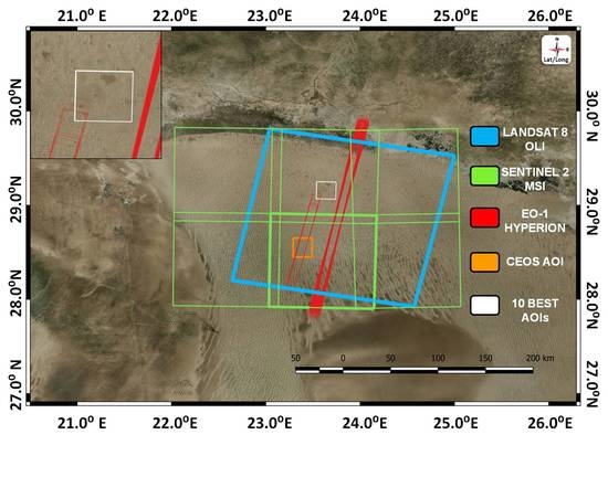
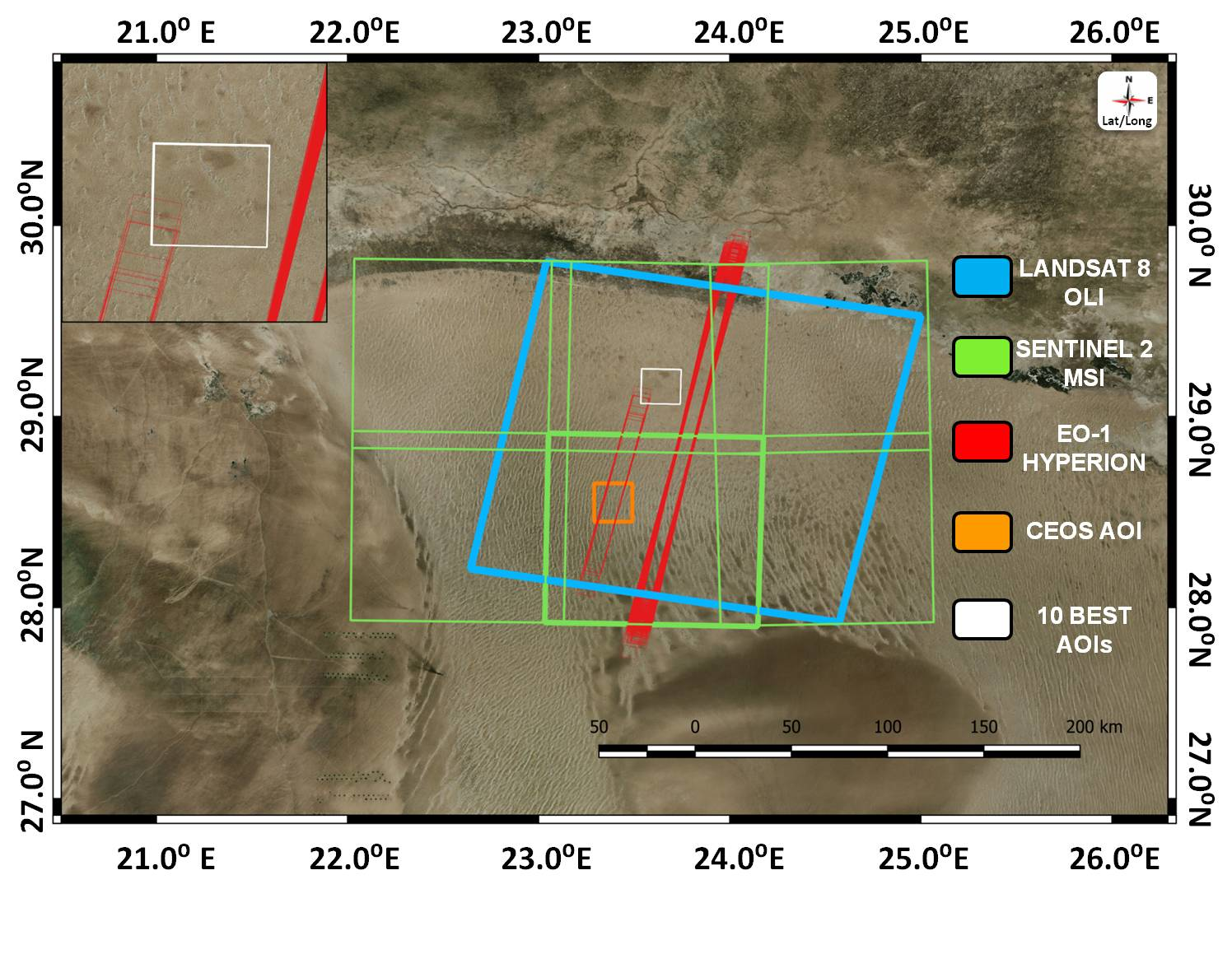
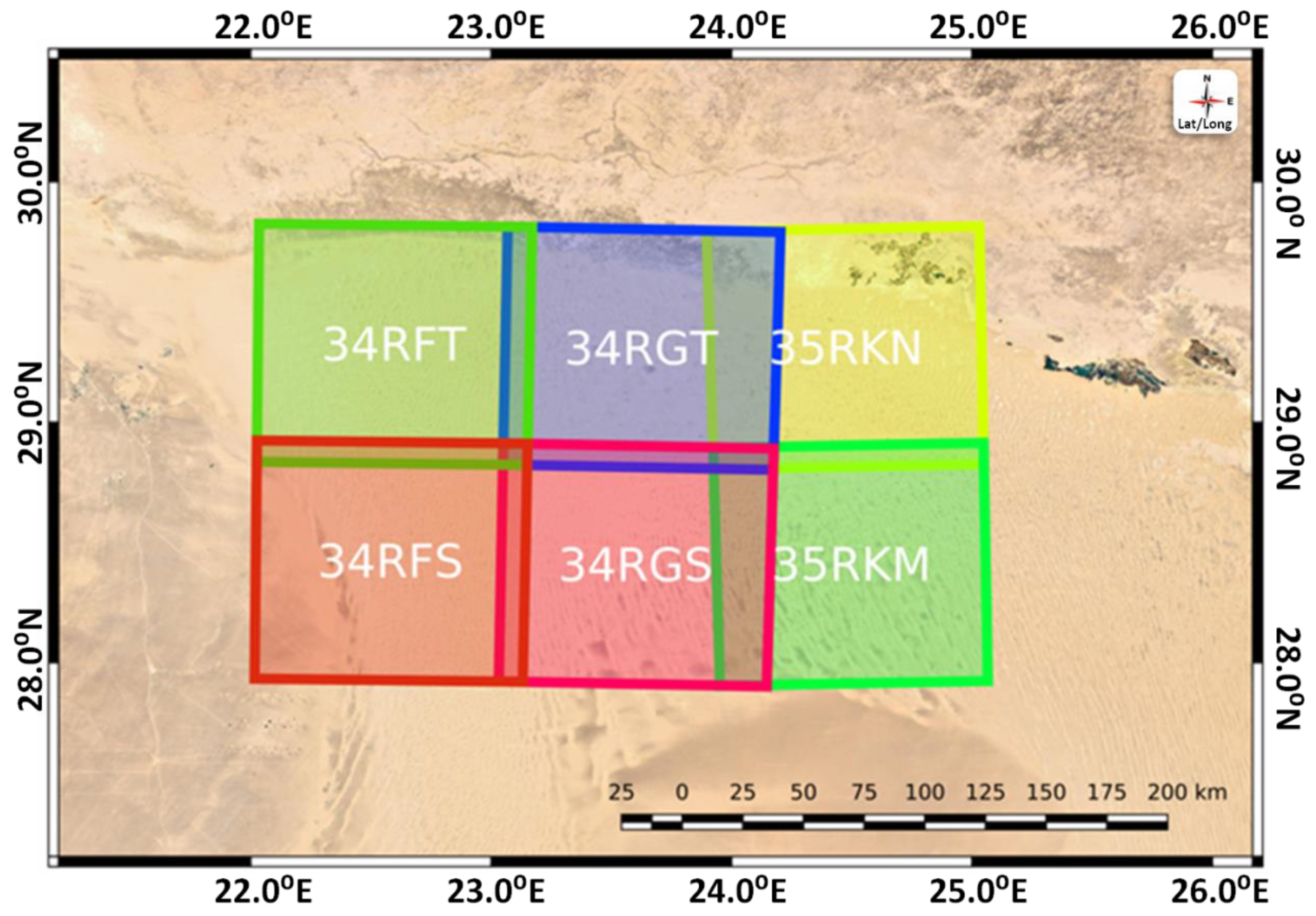
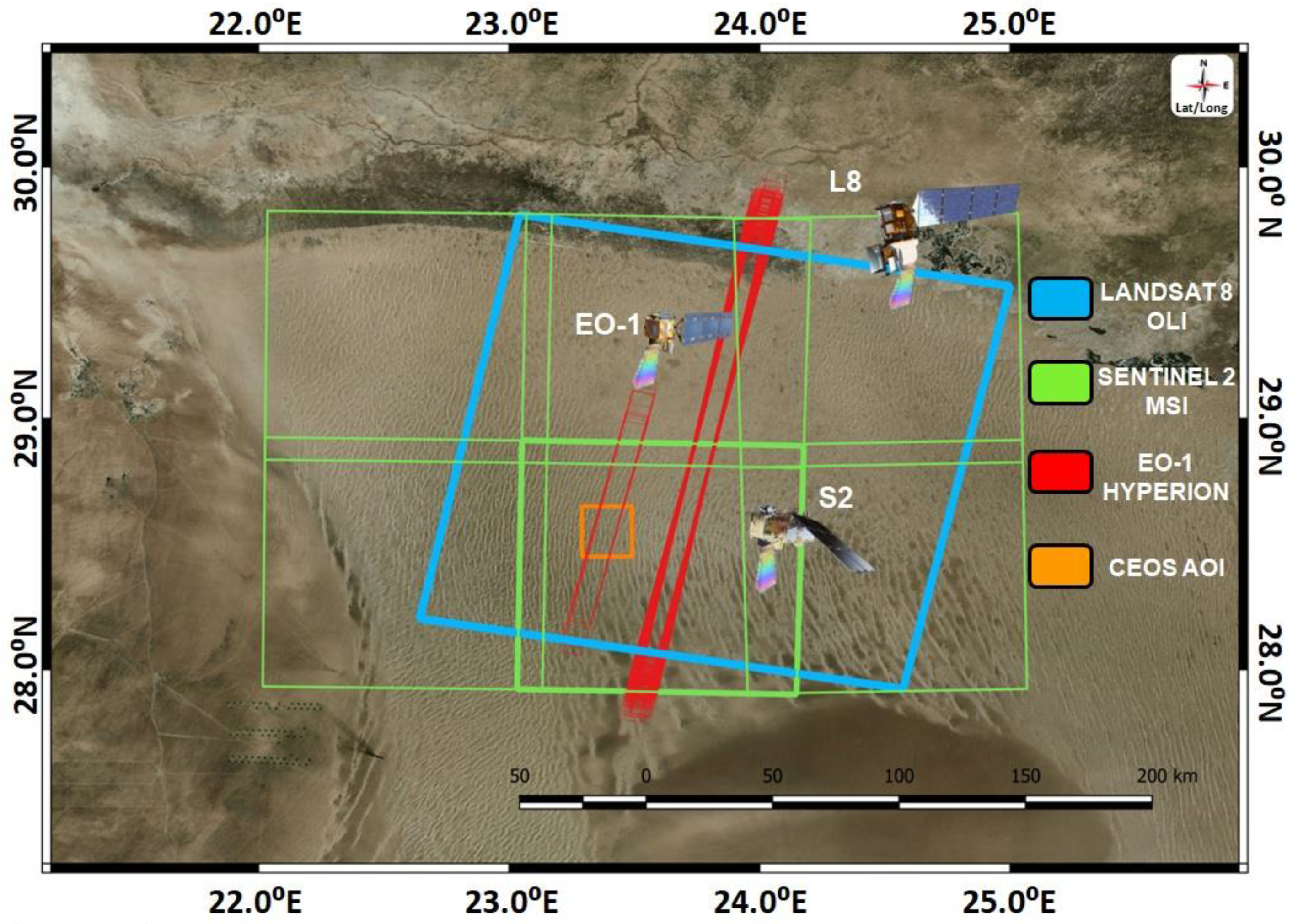
2.1. Study Area

Libya-4 was one of the six PICS recommended by the CEOS Working Group on Calibration and Validation (WGCV) [23] along with Mauritania-1, Mauritania-2, Algeria-3, Algeria-5, and Libya-1. It is located in the Great Sand Sea (28.55° N, 23.39° E) at an average height of 118 m above sea level. The study area was covered by unvegetated sand dunes and it usually had high atmospheric stability with low aerosol content as well as a low presence of cloudiness [24].

Libya-4 met all the characteristics of a good PICS [8]: Low reflectance anisotropy, high surface reflectance, high spatial and temporal uniformity, and a large ground surface.

On L8-OLI, the Libya-4 CEOS site was located at path 181 and row 40 referenced in the Second Worldwide Reference System (WRS-2) [25] with an approximate scene area of 185 × 180 km² [26]. In order to completely cover the area of Libya-4 for S2-MSI, it was necessary to use 6 tiles (34RFT, 34RFS, 34RGT, 34RGS, 35RKN, and 35RKM), spatially referenced using the Military Grid Reference System (MGRS), with an approximate size per tile of 100 × 100 km² and 10 km of overlap (Figure 1) [27].

CEOS defined an AOI of 20 × 20 km² that allowed higher resolution sensors that could not cover the full area in order to have a more localized reference zone [16]. The AOI of L8 and the tile 34RGS of S2 contained the CEOS AOI.

In addition to the different AOIs mentioned above, the hyperspectral data set of the Hyperion sensor of the now-decommissioned EO-1 satellite was taken into account (Figure 2). These Hyperion data allowed for a better spectral characterization of the Libya-4 surface due to the 220 continuous spectral bands covering the visible near-infrared (VNIR) and Short-Wave Infrared (SWIR), ranging from 400 nm to 2500 nm with a spectral resolution of approximately 10 nm [28].

In this work, we sought a common OGT for L8 and S2, and for that reason, we used the data of the tile WRS-2 181/40 of L8, and for S2, the data of the 6 MGRS tiles (34RFT, 34RFS, 34RGT, 34RGS, 35RKN, and 35RKM), which specifically covered the L8 area plus a small buffer. L8 images were slightly bigger than the WRS-2 tile (Figure 2).

2.2. Satellite Sensors

In order to evaluate the spatial and temporal homogeneity of Libya-4, L8-OLI and S2-MSI data were selected for their excellent quality [27,29].

L8 was launched on February 11, 2013, from Vandenberg Air Force Base, with two payloads: The Operational Land Imager (OLI) and the Thermal Infrared Sensor (TIRS). The OLI instrument had 9 spectral bands in the VNIR and SWIR range with a spatial resolution of 30 m, except for the panchromatic band that had a resolution of 15 m. In this work, we used L8 Collection 1 Tier 1 calibrated top-of-atmosphere (TOA) reflectance products referenced to WRS-2 in the Universal Transverse Mercator projection (UTM/WGS84) for the red, green, blue, and near infrared NIR bands. This product was radiometrically and geometrically calibrated and orthorectified using ground control points and a digital terrain model. It performed very well when comparing long time series of data at pixel level [30]. In 2017, a reprocessing of the data for the Landsat series was carried out, creating the so-called Collection-1, which we have used in this work [31].

S2 was part of the Copernicus Programme of the European Commission for the study and knowledge of planet Earth. The S2 programme currently consists of two twin satellites (S2A and S2B) orbiting in the same plane with a phase difference of 180 degrees. S2A was launched on June 23, 2015, while S2B was launched on March 7, 2017. The MSI payload was carried on board each of the satellites. This optical instrument had 13 spectral bands covering the region of VNIR to SWIR with spatial resolutions of 10 m for bands 2, 3, 4, and 8 and 20 m for the bands 5, 6, 7, 8A, 11, 12, and 60 m for the rest [27,32]. The blue, green, red, and NIR bands with a 10 m resolution were used for this work, corresponding, respectively, to the bands 2, 3, 4, and 8. It should be noted that S2 had two bands in the NIR spectral region, 8 and 8A, the latter being narrower with a spectral response close to the NIR band of Landsat 8. We used MSI’s wide NIR band (8) to maintain spatial consistency with the rest of the S2 bands. For S2 data, we employed the L1C product, which was structured in MGRS tiles of images of a size of 100 × 100 km² and were delivered in UTM/WGS84 projection. The images were in values of TOA reflectance multiplied by 10,000 [32].

The main characteristics of L8-OLI and S2-MSI bands are summarized in

Table 1. Satellite sensors, spectral bands, and spatial resolution characteristics.

	Band #	Band	Spatial Resolution (m)	Central Wavelength (nm)
Landsat 8 OLI	2	Blue	30	482.0
	3	Green	30	561.4
	4	Red	30	654.6
	5	NIR	30	864.7
Sentinel 2 A MSI	2	Blue	10	492.4
	3	Green	10	559.8
	4	Red	10	664.6
	8	NIR	10	832.8
Sentinel 2 B MSI	2	Blue	10	492.1
	3	Green	10	559.0
	4	Red	10	664.9
	8	NIR	10	832.9

.

2.3. Coefficient of Variation (CV)

We used the CV as an indicator of the radiometric homogeneity of Libya-4, both temporally and spatially. The CV is an operator that has been used as a measure of spatial homogeneity [33,34,35], as well as for the measurement of temporal homogeneity [36]. The CV can be defined as the quotient between the standard deviation and the average of values; therefore, it is a dimensionless unit that is usually represented as a percentage (Equation (1)).

$$CV=\frac{\sigma }{\left|\overline{x}\right|}$$

(1)

where $\left|\overline{x}\right|$ is the average value of the sample and σ is the standard deviation.

The Google Earth Engine was used to create the CV images of L8 and S2 data, given its cloud computing capacity and flexibility [37].

2.4. Spatial and Temporal Uniformity

In order to select and characterize the OGT on Libya-4 that met the criteria of greater spatial and temporal homogeneity, a long time series of data were used. The data from L8-OLI and S2-MSI sensors were used from the beginning of the missions until the last data available in 2018. The use of a human operator to reliably discern different types of clouds, shades, and other related elements present in the images has been proven to be fundamental in validating the quality of the images [38]. For this reason, datasets that show clouds, cloud shadows, suspended dust, and other obvious features that may negatively impact the analysis were filtered out by means of a quicklook photointerpretation, requiring the AOI to be covered by L8 in order to be visually clear. The use of a visual assessment to determine clouds, shadows, suspended dust, or other problematic elements was made due to the false positives that cloud detection algorithms present, especially for high-reflectance surfaces like deserts [39], along with the absence of thermal bands in S2 that made it difficult to generate a reliable cloud mask [40]. L8 quicklooks were downloaded from the Earth Resources Science and Observation Data Center (EROS) of the United States Geological Survey (USGS) and S2 quicklooks were from the Copernicus Hub. A total of 598 scenes from S2 and 64 scenes from L8 were used in the Google Earth Engine.

For the purposes of this work, we defined a coefficient in order to simultaneously study spatial and temporal homogeneity. We took the TOA reflectance image of the band i, of the acquisition j, and convolved it using the standard deviation operator and a 300 m square kernel to obtain the image ${\sigma }^{ij}$. The same process was repeated using the average operator to obtain the image ${\overline{x}}^{ij}$. Hence, after performing these spatial operations, there were two rasters per image band and the acquisitions, for computational convenience, were arranged in a data cube where the j axis (acquisition) represented the time component. The data was flattened across the time dimension and the image pairs were combined, following Equation (2), which defines the spatiotemporal CV (CV_ST).

$${C{V}_{\mathrm{ST}}}_{nm}^i =\frac{\sqrt{{{\displaystyle \sum }}_{j=1}^J{\left({\sigma }_{nm}^{ij}\right)}^2}}{{{\displaystyle \sum }}_{j=1}^J{\overline{x}}_{nm}^{ij}}$$

(2)

Here, the presence of (n, m), the pixel coordinates, indicated that the operations were pixel-based. J is the number of acquisitions.

It is worth highlighting that these operations were not tied to any sensor specifically. They worked equally for L8-OLI and S2-MSI. For this reason, each sensor was considered independently, with the calculation performed for the specific bands of that sensor. It is also important to note that the convolutions that were previously performed reduced the impact that small geometric errors can produce on the pixel-based operations.

The CV_ST made comparable the homogeneity of different spectral bands. Figure 3 shows the workflow of Libya-4 spatial and temporal uniformity analysis, applied on the L8 NIR band.

Once L8 and S2 Red, Green, Blue, and NIR (RGBNIR) CV_ST images were generated, a quasi-Newton optimization algorithm [41], known as the Limited Memory Broyden Fletcher Goldfarb Shanno (LM BFGS) method, was combined with the Basin–Hopping Global Optimization Technique (BH-GOT) [42] to narrow down the study area, focusing the analysis on the square zones with lower average CV_ST for each band. This optimization technique allowed for a function to be minimized. The algorithm implemented for this step minimized the average CV_ST in a square area where the bidimensional coordinates of its center and its side length were degrees of freedom. Hence, the optimization results provided the location and size of the squares with lower average CV_ST. The bidimensional coordinates “hop” across the WGS-2 path 181 and row 40 tile, which included the Libya-4 AOI, while the area fluctuated from a minimum of 20 × 20 km² (Figure 4), large enough to avoid the dune effect identified by Govaerts [17] and maximum of 100 × 100 km². This optimization technique has been applied in different areas such as physics, chemistry, mathematics, and biology [22,43,44,45].

Considering each band individually, we divided the optimized geometries into five classes, based on the CV_ST, and selected those that had the lowest CV_ST values so that they were categorized into the first class [46]. As the areas were grouped (Figure 4), it was possible to perform a geometric union of all of them, followed by the creation of a bounding box (Figure 5).

The bounding box contained the best areas identified for each spectral band and was then small enough to execute a brute-force CV_ST calculation on all bands simultaneously, using a square moving window of variable size and the average operator. The window was set to move in 30 m steps and had a minimum size of 20 × 20 km². This operation allowed us to select the AOIs with the lowest CV_ST in all the bands and sensors simultaneously (Figure 6). Using an average operator was feasible since the histograms for each spectral band for the CV_ST images were so similar that the band weights on average could be considered balanced, as shown in the Results Section below.

The general workflow and the intermediate processes performed to establish a location and size of the OGT is shown in Figure 7.

3. Results

The spatial and temporal homogeneity of Libya-4, expressed by the CV_ST for each Red-Green-Blue-near infrared RGBNIR band of L8 and S2, is presented in Figure 8 and Figure 9 and shows the maximum and minimum CV_ST values of each band in a color scale. The Western and central zones of the selected L8 and S2 AOI presented a lower CV_ST, and therefore, greater spatial and temporal uniformity, whereas the Northern zone had the highest CV_ST values, meaning that these areas were the least homogeneous. Independently of the band or sensor, the results of CV_ST on Libya-4 identified the most and least homogeneous areas. The average values in the CV_ST range for L8 were approximately 3.147% in the blue band and 3.641% in the red band. For S2, the mean CV_ST values were in the range of 3.734% for the blue band to 4.210% for the red band. For both satellites, the lowest average CV_ST and standard deviation corresponded to the blue band and the highest average CV_ST value and standard deviation with the red band.

Table 2. Average CV_ST for each band of L8 and S2 in the study AOI of Libya 4.

	Band	CVST Average (%)	CVST Standard Deviation (%)
Landsat 8	NIR	3.576	1.808
	Red	3.641	1.725
	Green	3.632	1.731
	Blue	3.147	1.661
Sentinel 2	NIR	4.184	2.552
	Red	4.210	2.360
	Green	4.114	2.139
	Blue	3.734	1.965

shows the average Libya-4 AOIs CV_ST values of each band, sensor, and standard deviation. The CV_ST standard deviation ranged from 1.661% to 1.808% for L8 and from 1.965% to 2.552% for S2. The minimum values were obtained in the blue band and the maximum values in the NIR band for both sensors.

For each RGBNIR band of L8 and S2, the best AOI class obtained after the classification of the CV_ST optimization is shown in Figure 10 and Figure 11. Each AOI had a different size with a minimum extension of 20 × 20 km². The lower the color transparency, the lower the average CV_ST of the AOI. The optimized AOIs of all bands were distributed in a relatively small area in the middle and lower zone of the 34RGT MGRS tile. This visually coincided with the CV_ST distribution values in Figure 8 and Figure 9. It is also worth mentioning that the optimized areas were also very similar across bands.

The similarity of the results obtained from each of the sensors provides evidence that the CV_ST is a good indicator for the location of homogeneous areas in Libya-4.

Table 3. Percentage of the average CV_ST value for the five best AOIs of each band and sensor.

	AOI	CVST Average (%) NIR Band	CVST Std. Dev. (%) NIR Band	CVST Average (%) Red Band	CVST Std. Dev. (%) Red Band	CVST Average (%) Green Band	CVST Std. Dev. (%) Green Band	CVST Average (%) Blue Band	CVST Std. Dev. (%) Blue Band
Landsat 8	1	2.3510	1.1615	2.4431	1.0869	2.2977	1.0346	1.8308	0.7565
	2	2.3573	1.1822	2.4473	1.0591	2.3040	0.9579	1.8334	0.8175
	3	2.3625	1.1671	2.4515	1.0350	2.3052	1.0286	1.8357	0.7658
	4	2.3681	1.1661	2.4535	1.0318	2.3106	1.0722	1.8361	0.8089
	5	2.3753	1.0799	2.4555	1.1019	2.3164	0.9422	1.8362	0.8332
Sentinel 2	1	2.6760	1.2922	2.7319	1.2942	2.5270	1.1236	2.1563	0.8760
	2	2.6790	1.3244	2.7342	1.2216	2.5274	1.1132	2.1563	0.8793
	3	2.6799	1.3185	2.7347	1.1861	2.5299	1.1326	2.1575	0.9828
	4	2.6829	1.3274	2.7408	1.2067	2.5361	1.2476	2.1583	0.9207
	5	2.6836	1.3126	2.7412	1.3170	2.5394	1.2239	2.1583	0.8930

and

Table 4. Area in km² of the five best AOIs of each band and sensor.

	AOI	Area km2 (Ellipsoidal, WGS84) NIR Band	Area km2 (Ellipsoidal, WGS84) Red Band	Area km2 (Ellipsoidal, WGS84) Green Band	Area km2 (Ellipsoidal, WGS84) Blue Band
Landsat 8	1	423.693	401.722	416.296	408.967
	2	404.103	416.332	406.534	413.851
	3	416.300	409.028	411.396	428.676
	4	446.283	433.745	404.106	411.407
	5	456.528	413.842	406.564	406.535
Sentinel 2	1	422.050	408.149	413.845	438.705
	2	403.300	406.536	403.303	445.454
	3	425.354	408.151	437.021	402.498
	4	422.875	429.506	405.719	417.120
	5	435.345	413.844	431.163	416.306

show the average CV_ST, its standard deviation, and the area for the five best AOIs of each band and sensor.

The number of AOIs used to generate the bounding box was four in NIR, three in red (2 outliers removed), six in green and blue bands for L8 and 13 in NIR for S2, eight in red, six in green, and twelve in blue band. On the fraction of the Libya-4 area defined by the bounding box, the brute-force search described in Section 2.4 was performed. The bands had similar distributions of values and therefore an unweighted average was appropriate for the average calculation and can be justified using Figure 12.

The brute-force algorithm iteratively swiped the bounding box area searching for a minimum average CV_ST, and similarly to BH-GOT with three variables and a minimum of 20 × 20 km², but this time the area searched was within the bounding box and the maximum square size was the bounding box size. The square center step and square side length were 30 m. Figure 13 and

Table 5. Features of the 10 best AOIs that were the result of the brute-force algorithm.

	AOI	CVST Average (%)	CVST Standard Deviation (%)	Area km2 (Elipsoidal, WGS84)	AOI Side Size (km)
AOIs Common Landsat 8 & Sentinel 2	1	2.3778	1.0368	400.000	20.000
	2	2.3779	1.0366	401.201	20.030
	3	2.3780	1.0367	402.404	20.060
	4	2.3782	1.0368	403.608	20.090
	5	2.3783	1.0358	404.814	20.120
	6	2.3785	1.0360	406.023	20.150
	7	2.3786	1.0377	407.232	20.180
	8	2.3787	1.0376	408.444	20.210
	9	2.3789	1.0378	409.658	20.240
	10	2.3790	1.0372	410.873	20.270

show the location, size, and CV_ST that resulted from the brute-force process. The 10 best AOIs found were very similar in their spatial location, average CV_ST, and surface. Figure 14 shows the best CV_ST found for each square side length.

We can now define the OGT as the AOI with the minimum average CV_ST. The chosen AOI avoids the dune effect, with an area of 20 × 20 km² and is completely contained in the Libya-4 AOI. It has the following coordinates (

Table 6. OGT corner coordinates in the UTM 34 N, WGS84 projection.

OGT Corner	Easting (m)	Northing (m)
Lower Left	746,850	3,218,250
Lower Right	766,860	3,218,250
Upper Right	766,860	3,238,230
Upper Left	746,850	3,238,230

):

It has an average CV_ST in the order of 2.5% for the NIR, red, and green bands, while it is close to 2% for the blue band, significantly better than the values obtained on the CEOS AOI, which are in the 3%–4% range for the visible near-infrared (VNIR) bands (

Table 7. Average CV_ST values for the L8 and S2 band on OGT and Committee on Observation Satellites System (CEOS) area.

	NIR Band CVST (%)	Red Band CVST (%)	Green Band CVST (%)	Blue Band CVST (%)
CEOS Zone Landsat 8	3.5151	3.3724	3.2194	2.7248
OGT Landsat 8	2.3561	2.4539	2.3047	1.8308
CEOS Zone Sentinel 2	4.1590	3.9481	3.6733	3.2507
OGT Sentinel 2	2.6698	2.7297	2.5192	2.1585

).

The comparison between the average CV_ST values of the OGT and the CEOS zone allows us to compare the fitness of this OGT for its use in post-launch radiometric performance and cross-calibration tasks. Both the CEOS AOI and the OGT have an area of 20 × 20 km², which means that the size of the AOI is not an influential factor in the comparison. Values for both areas are shown in Table 7.

Figure 14 shows the relationship between the average CV_ST of the best AOI, determined by the brute-force algorithm for a given side length. This shows a near-linear relationship, with two zones showing a negative relationship in which the average CV_ST decreases despite the increase of the AOI area (Figure 14).

4. Discussion

The PICS have been used over the last decades for absolute calibration, cross-calibration, and radiometric trend monitoring, as suggested by CEOS [9,10,11,47], and Libya-4 is one of the most widely used. It was initially defined for low to medium resolution sensors. Since S2-MSI and L8-OLI are high-resolution sensors, it was necessary to define a smaller and more homogeneous area with the purpose of reducing the uncertainties of the methodologies based on Libya-4 data. To meet this requirement, CEOS defined a smaller area within Libya-4.

Taking advantage of S2-MSI and L8-OLI data availability, we revisited the problem of defining a smaller area using a thorough methodology based on the use of a long time series of data from both sensors combined and a set of numeric methods. The data combination defined as CV_ST (Equation (2)) and the use of a global optimization technique allowed us to identify an area, namely OGT, which has ~1.5 times better spatio-temporal homogeneity than the CEOS AOI (Table 7) for all bands and more appreciable differences in L8 and S2 NIR bands. The variations of CV_ST between zones are higher in comparison with S2 data, which is probably a consequence of its higher spatial resolution that makes it more sensitive to spatial variations.

CV_ST images are very similar regardless of the band and sensor, indicating that the coefficient, as defined, is a good metric of the spatio-temporal homogeneity. The indication is confirmed after the optimization process. The barycentre of the best square areas found by the algorithms are located very close to each other. A significant number of them intersect for almost their entire surface, which highlights the robustness of this methodology.

While not used in this study, it is worth mentioning that there are data for the Hyperion sensor over this OGT. Hyperion is a hyperspectral instrument and its data could further enhance sensor comparison through the spectral band adjustment factor (SBAF) [48].

In general, the relationship between the CV_ST and the AOI side size follows a linear trend, which is broken twice when the area created by the brute-force algorithm engulfs very high and low CV_ST spots (Figure 14).

The OGT (AOI #1 in Table 5) has a CV_ST of 2.377% and an square side length of ~20 km, while the worst one found by the brute-force algorithm has a CV_ST of 2.485%, not far from the best value, but with a side length of ~29.3 km (Figure 14), corresponding to the minimum side length of the bounding box. The low CV_ST values obtained demonstrate the low spatio-temporal uncertainty of the study area where the OGT is located.

5. Conclusions

We have found that, in general, the average CV_ST improves as the surface is reduced. The brute-force algorithm consistently yields areas with surfaces close to the minimum of 20 × 20 km² set to avoid the dune effect.

The OGT defined here is a square area of ~20 × 20 km². The CEOS AOI, with the same area, yields CV_ST values in the range of 2.73%–4.16%, while the OGT range is 1.83%–2.73%. The results show that the new OGT performs significantly better in terms of homogeneity than the CEOS AOI, further reinforcing the possible use of this area for sensor cross-calibration and trend monitoring.

While this work has been done using L8 and S2 data, we do not consider that the OGT usage should be limited to OLI and MSI. On the contrary, the uniformity, which the area shows, can be an advantage for other optical sensors with similar resolutions, especially for those with no on-board calibration devices. Very high-resolution sensors, which typically have narrow swaths, can also have the benefit of using smaller and well-defined areas with the best uniformity.

We also consider that the methodology could be applicable to find OGTs within other PICS and Extended Pseudo Invariant Calibration Sites EPICS.

References

1. NOAA. Advisory Committee on Commercial Remote Sensing (ACCRES). Available online: https://www.nesdis.noaa.gov/CRSRA/pdf/AACRES_meeting_2018_Euroconsult.pdf (accessed on 14 November 2019).
2. Denis, G.; Claverie, A.; Pasco, X.; Darnis, J.P.; de Maupeou, B.; Lafaye, M.; Morel, E. Towards disruptions in Earth observation? New Earth Observation systems and markets evolution: Possible scenarios and impacts. Acta Astronaut. 2017, 137, 415–433. [Google Scholar] [CrossRef]
3. Vescovi, F.D.; Lankester, T.; Coleman, E.; Ottavianelli, G. Harmonisation initiatives of Copernicus data quality control. In Proceedings of the International Archives of the Photogrammetry, Remote Sensing and Spatial Information Sciences; 36th International Symposium on Remote Sensing of Environment, Berlin, Germany, 11–15 May 2015; Volume XL-7/W3. [Google Scholar]
4. Mhangara, P.; Mapurisa, W. Multi-Mission Earth Observation Data Processing System. Sensors 2019, 19, 3831. [Google Scholar] [CrossRef] [PubMed] [Green Version]
5. Chander, G.; Haque, M.O.; Sampath, A.; Brunn, A.; Trosset, G.; Hoffmann, D.; Roloff, S.; Thiele, M.; Anderson, C. Radiometric and geometric assessment of data from the RapidEye constellation of satellites. Int. J. Remote Sens. 2013, 34, 5905–5925. [Google Scholar] [CrossRef]
6. Lyapustin, A.; Wang, Y.; Xiong, X.; Meister, G.; Platnick, S.; Levy, R.; Hall, F. Scientific impact of MODIS C5 calibration degradation and C6+ improvements. Atmos. Meas. Tech. 2014, 7, 4353–4365. [Google Scholar] [CrossRef] [Green Version]
7. Cosnefroy, H.; Leroy, M.; Briottet, X. Selection and characterization of Saharan and Arabian desert sites for the calibration of optical satellite sensors. Remote Sens. Environ. 1996, 58, 101–114. [Google Scholar] [CrossRef]
8. Chander, G. Catalog of worldwide test sites for sensor calibration. In Proceedings of the JACIE Workshop 2008, Fairfax, VA, USA, 26–28 March 2008. [Google Scholar]
9. Mishra, N.; Helder, D.; Angal, A.; Choi, J.; Xiong, X. Absolute calibration of optical satellite sensors using Libya 4 pseudo invariant calibration site. Remote Sens. 2014, 6, 1327–1346. [Google Scholar] [CrossRef] [Green Version]
10. Mishra, N.; Haque, M.O.; Leigh, L.; Aaron, D.; Helder, D.; Markham, B. Radiometric cross calibration of Landsat 8 operational land imager (OLI) and Landsat 7 enhanced thematic mapper plus (ETM+). Remote Sens. 2014, 6, 12619–12638. [Google Scholar] [CrossRef] [Green Version]
11. Angal, A.; Xiong, X.X.; Choi, T.; Chander, G.; Mishra, N.; Helder, D.L. Impact of Terra MODIS Collection 6 on long-term trending comparisons with Landsat 7 ETM+ reflective solar bands. Remote Sens. Lett 2013, 4, 873–881. [Google Scholar] [CrossRef]
12. ESA. Radiometric Calibration Workshop for European Missions. Available online: https://earth.esa.int/documents/700255/3194632/B%2B%C2%AEatrice+Berthelot_PICSCAR-PPT-022-MAGv1.0_BBerthelot_PHenry_20170830.pdf/9ddad0e8-532c-4f6c-9f19-404c8280755c (accessed on 14 November 2019).
13. Sterckx, S.; Livens, S.; Adriaensen, S. Rayleigh, deep convective clouds, and cross-sensor desert vicarious calibration validation for the PROBA-V mission. IEEE Trans. Geosci. Remote Sens. 2013, 51, 1437–1452. [Google Scholar] [CrossRef]
14. Govaerts, Y.M.; Clerici, M.; Clerbaux, N. Operational calibration of the Meteosat radiometer VIS band. IEEE Trans. Geosci. Remote Sens. 2004, 42, 1900–1914. [Google Scholar] [CrossRef]
15. Bhatt, R.; Doelling, D.R.; Wu, A.; Xiong, X.; Scarino, B.R.; Haney, C.O.; Gopalan, A. Initial stability assessment of S-NPP VIIRS reflective solar band calibration using invariant desert and deep convective cloud targets. Remote Sens. 2014, 6, 2809–2826. [Google Scholar] [CrossRef] [Green Version]
16. Lacherade, S.; Fougnie, B.; Henry, P.; Gamet, P. Cross calibration over desert sites: Description, methodology, and operational implementation. IEEE Trans. Geosci. Remote Sens. 2013, 51, 1098–1113. [Google Scholar] [CrossRef]
17. Govaerts, Y.M. Sand Dune Ridge Alignment Effects on Surface BRF over the Libya-4 CEOS Calibration Site. Sensors 2015, 15, 3453–3470. [Google Scholar] [CrossRef] [PubMed] [Green Version]
18. Tuli, F.T.Z.; Pinto, C.T.; Angal, A.; Xiong, X.; Helder, D. New Approach for Temporal Stability Evaluation of Pseudo-Invariant Calibration Sites (PICS). Remote Sens. 2019, 11, 1502. [Google Scholar] [CrossRef] [Green Version]
19. Broyden, C.G. The Convergence of a Class of Double-rank Minimization Algorithms 1. General Considerations. IMA J. Appl. Math. 1970, 6, 76–90. [Google Scholar] [CrossRef]
20. Fletcher, R. A new approach to variable metric algorithms. Comput. J. 1970, 13, 317–322. [Google Scholar] [CrossRef] [Green Version]
21. Shanno, D.F. Conditioning of Quasi-Newton methods for function minimization. Math. Comput. 1970, 24, 647–656. [Google Scholar] [CrossRef]
22. Wales, D.J.; Doye, J.P.K. Global Optimization by Basin-Hopping and the Lowest Energy Structures of Lennard-Jones Clusters Containing up to 110 Atoms. J. Phys. Chem. A 1997, 101, 5111. [Google Scholar] [CrossRef] [Green Version]
23. Teillet, P.; Chander, G. Terrestrial reference standard sites for postlaunch sensor calibration. Can. J. Remote Sens. 2010, 36, 437–450. [Google Scholar] [CrossRef]
24. Choi, T.J.; Xiong, X.; Angal, A.; Chander, G.; Qu, J.J. Assessment of the spectral stability of Libya 4, Libya 1, and Mauritania 2 sites using Earth Observing One Hyperion. J. Appl. Remote Sens. 2014, 8, 083618. [Google Scholar] [CrossRef]
25. USGS. Remote Sensing Technologies. CalVal Portal. Available online: https://calval.cr.usgs.gov/apps/libya-4 (accessed on 3 October 2019).
26. USGS. Version 4.0 Landsat 8 Data Users Handbook. Available online: https://www.usgs.gov/media/files/landsat-8-data-users-handbook (accessed on 3 October 2019).
27. Gascon, F.; Bouzinac, C.; Thépaut, O.; Jung, M.; Francesconi, B.; Louis, J.; Lonjou, V.; Lafrance, B.; Massera, S.; Gaudel-Vacaresse, A.; et al. Copernicus Sentinel-2A Calibration and Products Validation Status. Remote Sens. 2017, 9, 584. [Google Scholar] [CrossRef] [Green Version]
28. USGS. Earth Observing 1 (EO-1). Available online: https://eo1.usgs.gov/ (accessed on 3 October 2019).
29. Roy, D.; Wulder, M.; Loveland, T.; Woodcock, C.; Allen, R.; Anderson, M.; Helder, D.; Irons, J.; Johnson, D.; Kennedy, R.; et al. Landsat-8: Science and product vision for terrestrial global change research. Remote Sens. Environ. 2014, 145, 154–172. [Google Scholar] [CrossRef] [Green Version]
30. USGS. Landsat Collection 1. Available online: https://www.usgs.gov/land-resources/nli/landsat/landsat-collection-1?qt-science_support_page_related_con=1#qt-science_support_page_related_con (accessed on 3 October 2019).
31. Dwyer, J.L.; Roy, D.P.; Sauer, B.; Jenkerson, C.B.; Zhang, H.K.; Lymburner, L. Analysis Ready Data: Enabling Analysis of the Landsat Archive. Remote Sens. 2018, 10, 1363. [Google Scholar] [CrossRef]
32. ESA. Sentinel-2. Available online: https://sentinel.esa.int/web/sentinel/missions/sentinel-2 (accessed on 4 October 2019).
33. Kneubühler, M.; Schaepman, M.E.; Thome, K. Long-Term Vicarious Calibration Efforts of MERIS at Railroad Valley playa (Nevada)—An update. In Proceedings of the Second Working Meeting on MERIS and AATSR Calibration and Geophysical Validation (MAVT-2006), Frascati, Italy, 20–24 March 2006. [Google Scholar]
34. Devries, C.; Danaher, T.; Denham, R.; Scarth, P.; Phinn, S. An operational radiometric calibration procedure for the Landsat sensors based on pseudo-invariant target sites. Remote Sens. Environ. 2007, 107, 414–429. [Google Scholar] [CrossRef]
35. Gu, X.; Guyot, G.; Verbrugghe, M. Analyze de la variabilité spatiale d’un site-test: Exemple de “La Crau” (France). Photo Interpret. 1990, 1, 39–52. [Google Scholar]
36. Helder, D.L.; Basnet, B.; Morstad, D.L. Optimized identification of worldwide radiometric pseudo-invariant calibration sites. Can. J. Remote Sens. 2010, 36, 527–539. [Google Scholar] [CrossRef]
37. Gorelick, N.; Hancher, M.; Dixon, M.; Ilyushchenko, S.; Thau, D.; Moore, R. Google Earth Engine: Planetary-scale geospatial analysis for everyone. Remote Sens. Environ. 2017, 202, 18–27. [Google Scholar] [CrossRef]
38. Coluzzi, R.; Imbrenda, V.; Lanfredi, M.; Simoniello, T. A first assessment of the Sentinel 2 Level 1-C cloud mask product to support informed surface analyses. Remote Sens. Environ. 2018, 217, 426–443. [Google Scholar] [CrossRef]
39. Sun, L.; Mi, X.; Wei, J.; Wang, J.; Tian, X.; Yu, H.; Gan, P. A cloud detection algorithm-generating method for remote sensing data at visible to short-wave infrared wavelengths. ISPRS J. Photogramm. Remote Sens. 2017, 124, 70–88. [Google Scholar] [CrossRef]
40. Helder, D.; Markham, B.; Morfitt, R.; Storey, J.; Barsi, J.; Gascon, F.; Clerc, S.; LaFrance, B.; Masek, J.; Roy, D.P.; et al. Observations and Recommendations for the Calibration of Landsat 8 OLI and Sentinel 2 MSI for Improved Data Interoperability. Remote Sens. 2018, 10, 1340. [Google Scholar] [CrossRef] [Green Version]
41. Battiti, R.; Masulli, F. BFGS optimization for faster and automated supervised learning. In Proceedings of the International Neural Network Conference, Paris, France, 9–13 July 1990; Springer: Dordrecht, The Netherlands, 1990; pp. 757–760. [Google Scholar]
42. Iwamatsu, M.; Okabe, Y. Basin hopping with occasional jumping. Chem. Phys. Lett. 2004, 399, 396–400. [Google Scholar] [CrossRef] [Green Version]
43. Wales, D. Energy Landscapes: Applications to Clusters, Biomolecules and Glasses; Cambridge University Press: Cambridge, UK, 2003. [Google Scholar]
44. Li, Z.; Scheraga, H.A. Monte Carlo-minimization approach to the multiple-minima problem in protein folding. Proc. Natl. Acad. Sci. USA 1987, 84, 6611–6615. [Google Scholar] [CrossRef] [PubMed] [Green Version]
45. Wales, D.J.; Scheraga, H.A. Global Optimization of Clusters, Crystals, and Biomolecules. Science 1999, 285, 1368–1372. [Google Scholar] [CrossRef] [PubMed] [Green Version]
46. Jenks, G.F. The data model concept in statistical mapping. Int. Yearb. Cartogr. 1967, 7, 186–190. [Google Scholar]
47. Uprety, S.; Cao, C. Suomi NPP VIIRS reflective solar band on-orbit radiometric stability and accuracy assessment using desert and Antarctica Dome C sites. Remote Sens. Environ. 2015, 166, 106–115. [Google Scholar] [CrossRef]
48. Chander, G.; Mishra, N.; Helder, D.L.; Aaron, D.B.; Amit, A.; Choi, T.; Doelling, D.R. Applications of Spectral Band Adjustment Factors (SBAF) for cross-calibration. IEEE Trans. Geosci. Remote Sens. 2013, 51, 1267–1281. [Google Scholar] [CrossRef]
Figure 1. Google Earth view of the S2 tiles in the study area.
Remotesensing 11 02909 g001
Figure 2. Google Earth representation with the location of the different L8 and S2 areas of interest (AOI), as well as the acquisition zones of the Hyperion sensor on Libya-4.
Remotesensing 11 02909 g002
Figure 3. L8-Operational Land Imager near infrared OLI NIR band example of the spatial and temporal Coefficient of Variation (CV) calculation workflow.
Remotesensing 11 02909 g003
Figure 4. NIR, red, green, and blue Libya-4 AOIs of S2 and L8 found by optimization.
Remotesensing 11 02909 g004
Figure 5. (A) Selection of the best AOIs for each band and sensor. (B) Geometric union. (C) Bounding box.
Remotesensing 11 02909 g005
Figure 6. Workflow for the Optimized Ground Target (OGT) location within the bounding box.
Remotesensing 11 02909 g006
Figure 7. General workflow for the OGT location on Libya-4.
Remotesensing 11 02909 g007
Figure 8. L8 average CVST for Red-Green-Blue-near infrared RGBNIR bands on Libya-4. Note that the image is slightly bigger than the WRS-2 tile.
Remotesensing 11 02909 g008
Figure 9. S2 average CVST for RGBNIR bands on Libya-4.
Remotesensing 11 02909 g009
Figure 10. Location of the lowest CVST AOI class for each L8 RGBNIR band.
Remotesensing 11 02909 g010
Figure 11. Location of the lowest CVST AOI class for each S2 RGBNIR band.
Remotesensing 11 02909 g011
Figure 12. Normalized bands histogram in the bounding box.
Remotesensing 11 02909 g012
Figure 13. Layout of AOIs within Libya-4.
Remotesensing 11 02909 g013
Figure 14. Linear relationship between the average CVST and the side length of the square AOI, as well as the differentiated zones with decreasing trends.
Remotesensing 11 02909 g014