Article

Mapping at 30 m Resolution of Soil Attributes at Multiple Depths in Midwest Brazil

by
Raúl R. Poppiel
1,
Marilusa P. C. Lacerda
1,
José L. Safanelli
2,
Rodnei Rizzo
2,
Manuel P. Oliveira, Jr.
1,
Jean J. Novais
1 and
José A. M. Demattê
2,*
1
Faculty of Agronomy and Veterinary Medicine, Darcy Ribeiro University Campus, University of Brasília; ICC Sul, Asa Norte, Postal Box 4508, Brasília 70910-960, Brazil
2
Department of Soil Science, Luiz de Queiroz College of Agriculture, University of São Paulo; Pádua Dias Av., 11, Piracicaba, Postal Box 09, São Paulo 13416-900, Brazil
*
Author to whom correspondence should be addressed.
Remote Sens. 2019, 11(24), 2905; https://doi.org/10.3390/rs11242905
Submission received: 18 October 2019 / Revised: 26 November 2019 / Accepted: 3 December 2019 / Published: 5 December 2019

Abstract

:
The Midwest region in Brazil has the largest and most recent agricultural frontier in the country where there is no currently detailed soil information to support the agricultural intensification. Producing large-extent digital soil maps demands a huge volume of data and high computing capacity. This paper proposed mapping surface and subsurface key soil attributes with 30 m-resolution in a large area of Midwest Brazil. These soil maps at multiple depth increments will provide adequate information to guide land use throughout the region. The study area comprises about 851,000 km2 in the Cerrado biome (savannah) in the Brazilian Midwest. We used soil data from 7908 sites of the Brazilian Soil Spectral Library and 231 of the Free Brazilian Repository for Open Soil Data. We selected nine key soil attributes for mapping and aggregated them into three depth intervals: 0–20, 20–60 and 60–100 cm. A total of 33 soil predictors were prepared using Google Earth Engine (GEE), such as climate and geologic features with 1 km-resolution, terrain and two new covariates with 30 m-resolution, based on satellite measurements of the topsoil reflectance and the seasonal variability in vegetation spectra. The scorpan model was adopted for mapping of soil variables using random forest regression (RF). We used the model-based optimization by tuning RF hyperparameters and calculated the scaled permutation importance of covariates in R software. Our results were promising, with a satisfactory model performance for physical and chemical attributes at all depth intervals. Elevation, climate and topsoil reflectance were the most important covariates in predicting sand, clay and silt. In general, for predicting soil chemical attributes, climatic variables, elevation and vegetation reflectance provided to be the most important of predictive components, while for organic matter it was a combination of climatic dynamics and reflectance bands from vegetation and topsoil. The multiple depth maps showed that soil attributes largely varied across the study area, from clayey to sandy, suggesting that less than 44% of the studied soils had good natural fertility. We concluded that key soil attributes from multiple depth increments can be mapped using Earth observations data and machine learning methods with good performance.

Graphical Abstract

1. Introduction

Soil is a foundation for production systems, having capabilities for stabilizing the ecosystem [1]. Reliable spatial soil information can improve natural capital assessment, becoming important for food production, in large countries or emerging economies where the major demographic growth is expected [2]. Soil mapping is expensive and time-demanding, consequently performing adequate maps in large areas takes several years and require significant economic resources. Such fact is observed in countries like Brazil, which is covered by small scale soil maps, mostly developed by Brazilian government institutions using RADAMBRASIL (Radar on Amazon and Brazil) project data (1:1,000,000 or nominally 2 km) [3]. In this case, such maps are not capable of supporting any decision making in regional or local scales.
The huge volume of quantitative (pedometric) data required in the production of soil attribute maps, for large areas, limits the feasibility of conventional (traditional) manual (expert-based) soil mapping [3,4]. Several key soil factors are still not fully represented by classical environmental covariates, being necessary to develop new covariates that provide improved proxies for describing spatial soil variations. Advances in Earth observation (satellite images and products), digital elevation models and digital soil mapping (DSM) frameworks, based on machine learning and cloud-based computing, might be a solution to the lack of adequate soil data [5]. An Earth observation product that has raised attention in DSM is the satellite image. Such data can retrieve medium- to high-resolution information and are easily acquired. Recently, studies have employed multi-temporal images in soil assessment and mapping. Such data provides measurements of topsoil reflectance, which are directly related to clay content, organic matter, mineralogy, moisture and soil color [6]. The synergy between satellite images and DSM is described by Diek et al. [7], who performed a multi-temporal composite from the Airborne Prism Experiment (APEX). By overlapping images, the authors doubled the amount of bare surface pixels in the scene and presented an enhanced spatial representation of soil surface. Later, Diek et al. [8] developed a method for identifying the least-vegetated pixels (e.g., barest pixel) in a dense Landsat time series. Such data was used to estimate soil attributes and evaluate the contribution of remote sensing (RS) to conventional and digital soil-mapping procedures. Similarly, Rogge et al. [9] proposed the Soil Composite Mapping Processor (SCMaP), which is an approach able to use per-pixel compositing to address the issue of limited soil exposure. Another bare surface composition technique was proposed by Demattê et al. [10], called the Geospatial Soil System (GEOS3). These authors validated the method by comparing the bare surface data (described as SySI) to laboratory spectral measurements, and found a canonical correlation of 0.93. Later, Fongaro et al. [11] used such composite images to digitally map soils from southeastern Brazil. These authors described an expressive enhancement in clay content’s digital mapping when employing SySI and terrain derivatives. The R2 and root mean squared error (RMSE) improved from 0.64 and 93.44 g kg−1 to 0.83 and 65.36 g kg−1, respectively. Finally, Mendes et al. [12] indicated that besides surface layer mapping, SySI can also aid in the prediction of soil subsurface attributes.
The prediction in DSM is usually based on machine learning techniques, which fit models for the spatial prediction of soil variables (i.e., maps of soil attributes and classes at different resolutions) [4]. While machine learning supports the soil spatial predictions [13], cloud-based computing provides a superior architecture for the execution of such complex algorithms [14]. These techniques are very attractive, once it result in the automation of processes, reducing overall soil data production costs, combining statistics, data science, soil science, physical geography, remote sensing (RS), geoinformation science and a number of other sciences [3,5,10,13].
A brief search in literature regarding the terms “soil” and “machine learning” resulted in more than 72,000 publications, from which 7200 items were published in the first half of 2019 and 4000 discuss random forest (RF) algorithms. The RF algorithm was first introduced by Breiman (2001) and became a standard nonparametric classification and regression tool. The method establishes prediction rules based on various types of predictor variables, without making any prior assumption on the form of their association with the response variable [15]. The RF is one of most popular algorithms in DSM, being employed in several soil mapping studies [5,16,17,18,19]. Many inter-comparisons between machine learning algorithms are described in literature, and in most cases, authors indicated RF as the most adequate algorithm for digitally mapping soils. Keskin et al. [20] compared many models to quantify stochastic and/or deterministic components of soil carbon (C) pools. The prediction performance indicated the RF as the best algorithm. The covariables that best described variations in C pools were the biotic and hydro-pedological ones. Lithologic and climatic factors had a reasonable influence in C predictions, while topographic factors did not contribute to soil C modeling. Similarly, Nussbaum et al. [21] evaluated six approaches for digitally mapping 14 soil attributes at four depths. They found small differences in predictive performances, but RF was often the best among all methods. Hengl et al. [22] mapped 14 soil properties from African soils, combining quality-controlled point data and a large number of covariates. The random forest was the best method, outperforming linear regression with an average decrease of 15%–75% in RMSE across soil properties and depths.
In Brazil, there are no soil attribute maps with complete coverage across the Brazilian Midwest, which could support management and policy decisions. This region has the largest and most recent agricultural frontier in Brazil [23], which contributes about 34% and more than 10% to the agricultural production and gross domestic product of the country, respectively [24]. Thus, we intend to produce up-to-date maps of surface and subsurface key soil attributes in a large extension of the Midwest of Brazil. These maps at multiple depth increments might provide adequate information to conduct account for the multi-functionality of soil in the region. Therefore, our aims are to (a) define composite images (described hereafter as SySI and SyVI), which describes the reflectance variability of bare surfaces and natural vegetation; (b) employ SySI and SyVI along with terrain derivatives, geologic and climate variables as covariates in the digital mapping of key soil attributes in the Midwest Brazil; (c) evaluate the performance of the random forest algorithm, implemented in a cloud-based computing, to describe the spatial variability of soils from the study site; (d) identify the model covariates that were most relevant to describe the soil variability in Midwest Brazil. We expect that Earth observation data and machine learning, coupled with Brazilian available legacy soil datasets, to promote a favorable framework to produce accurate soil predictions for this important agricultural region. We assume that it is possible to map physical and chemical soil attributes for three standard depth intervals (0–20, 20–60 and 80–100 cm) with 30 m-resolution across the Midwest region in Brazil.

2. Material and Methods

2.1. Study Area and Soil Data

The study area comprises about 851,000 km2 in the Cerrado biome (savanna) in the Brazilian Midwest (Figure 1), with extensive plateaus covered by Cerrado vegetation and gallery forest. The climate is tropical humid, which has two well-defined seasons, wet in summer and dry in winter, with annual precipitation ranging from 1200 to 1800 mm. According to the 1:1,000,000-scale map of pedology [25], the Ferralsols, Lixisols, Plinthosols, Arenosols and Regosols [26] are dominant soils of the region, which developed from highly diversified lithologies, consisting of volcanic, metamorphic, and sedimentary rocks, who reworked surface materials [27].
We obtained soil data from 7908 sites of the Brazilian Soil Spectral Library (BSSL) [28] and 231 of the Free Brazilian Repository for Open Soil Data (FEBR) [29]. The BSSL started in 1995 as a collaborative network formed by several institutions all over Brazil. The FEBR contains legacy soil observations data collected by Brazilian government agencies since the 1960s.
We selected nine soil attributes for mapping in the study area (Figure 1), such as sand, silt and clay contents, organic matter ( O M = o r g a n i c   c a r b o n   × 1.72 ), pH measured in water (pH H2O) and in potassium chloride (pH KCl), cation exchange capacity ( C E C = C a 2 + + M g 2 + + K + + H + + A l 3 + ), and base saturation ( V % = ( ( C a 2 + + M g 2 + + K + ) × 100 ) ÷ C E C ) and aluminum saturation ( m % = ( A l 3 + × 100 ) ÷ ( C a 2 + + M g 2 + + K + + A l 3 + ) ) at 0–20 cm, 20–60 and 60–100 cm depth intervals. These soil attributes are commonly used (as key criteria) to guide agricultural recommendations, to evaluate the locations most suitable for farming and delineation of soil management zones. According to [30], maximum rooting depth of crops by far can exceed 100 cm soil depths. Tus, soil attributes from 0 to 100 cm depth can affect plant growth and yield. When exploring the complete dataset, we checked for possible duplicated data and typos. To remove outliers from the dataset before modelling, we used more than one condition by nesting IF functions in Microsoft Excel. For example, to remove sand, silt and clay contents smaller or greater than 1000 g kg−1 [=IF(SUM(Sand;Silt;Clay)=1000);“OK”;“REMOVE”)], or testing IF the relationships (V% vs. pH vs. m%, OM vs. CEC) were coherent. A large proportion of the data had information based on the laboratory method of Embrapa [31], while the remaining were transformed to the same standard units.
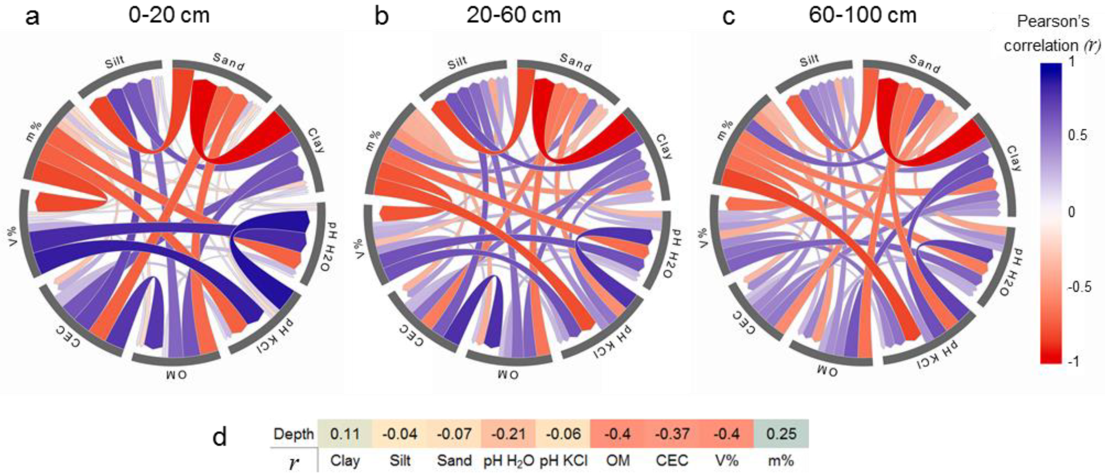
Finally, we performed a chord diagram based on Pearson correlation to check weighted relationships between soil attributes using the circlize package version 0.4.8 [32] in the R software [33]. In that diagram, each soil attribute is represented by a fragment on the outer part of the circular layout, where the size of the connections is proportional to the value of the correlation.
The framework used for digital mapping of soil attributes (Figure 2), was fully implemented via the cloud-based platform of Google Earth Engine (GEE) [14] and the R environment for statistical computing [33].

2.2. Preparing Soil Covariates

Soil covariate layers can be used as predictors (“independent variables”) in the statistical modelling. Their preparation is time and resources consuming, involving a huge image processing to transform large environmental databases into relevant predictors for machine learning of soil attributes. Therefore, efforts to produce appropriate predictors to explain the spatial distribution of soil attributes (at detail and generalization) increases the accuracy of the models. Various covariates (e.g., climate, terrain attributes and RS data) representing soil state factors have been widely used in statistical models to predict soil texture, bulk density, organic carbon, nutrients (Ca, Mg, K, Na, N, P), available water capacity, pH and CEC [4,17,22,34,35,36,37].
For mapping the selected soil attributes, a group of covariates were obtained (Table 1) to act as proxies for describing soil (s), climate (c), vegetation (o), relief (r), parent material (p), age of surface (a) and spatial position (n) in the scorpan prediction model [3], using the GEE [14]. A robust approach, for fitting single models using input data at multiple resolutions is to combine covariates (with different grid cell size) to a single, common resolution. However, no information gain is yield to the downscaled covariate. We defined the target grid resolution to 30 m that was in accordance with the majority of covariates used. We consider the inverse distance weighting (IDW) interpolator the most appropriate in our case to downscale the 1 km covariates (climate and geology) to 30 m resolution. This is because IDW attenuates the influence of distant points by its use of inverse distance weight given an assumption of positive spatial autocorrelation [38], and also because it is easy to be implemented and available in GEE [14]. Knowing that soils were formed in response to different forming processes operating over different ranges of distances or scales [3,39], the use of multi-resolution covariates may help the prediction models to capture the multi-scale soil spatial variations.

2.2.1. Climate Data

Annual temperature average, range and seasonality, and annual precipitation and seasonality values were obtained from the WorldClim dataset [40] at a spatial resolution of 1 km, and then were downscaled to 30 m pixel resolution by IDW. These data layers derived from numerous weather stations data interpolated by thin-plate smoothing spline, using latitude, longitude, and elevation as independent variables [40]. The WorldClim is the highest resolution continuous climate database available for the study region.

2.2.2. Relief and Geology Data

We derived local terrain attributes, including elevation, slope, aspect, horizontal and vertical curvature and topographic position index (TPI) from the 30 m ALOS digital elevation model [41] within GEE. Slope, aspect and curvatures, were calculated from the partial derivatives of terrain using a 3 × 3 moving window [42]. The TPI was calculated by subtracting the elevation in meters at a given location (or cell) to the mean elevation of all cells within a neighborhood specified by a radius of 3 km. Highly positive values are associated with peaks and ridges, while highly negative values are associated with valley bottoms and sinks. We obtained the density of geological lineaments by counting the meters of structural lines obtained from a 1:1,000,000-scale map [27] in 1 km grids, and then transformed to raster and downscaled to 30 m pixel resolution by the IDW method.

2.2.3. Landsat-Derived Data

Data. The Landsat program has been observing the Earth continuously from 1972 through the present day. We used Landsat surface reflectance data (Tier 1, Collection 1) of different sensors covering the study area from 1982 to 2019, including the Thematic Mapper (TM, Landsat 4–5), the Enhanced Thematic Mapper Plus (ETM+, Landsat 7), and the Operational Land Imager and Thermal Infrared Sensor (OLI/TIRS, Landsat 8) with 16 days revisiting time and 30 m resolutions [43,44]. Considering these products are gridded into common characteristics (resolution, projection, spatial extent, scale values and spectral ranges), we performed an inter-sensor harmonization to combine their separated collections into a single dataset. The bands of each sensor, positioned in equivalent spectral regions, were matched into a common name (e.g., Blue, Green, Red, NIR, SWIR1, SWIR2 and LST) using the specific band number (Table A1). The quality assessment bands were used to remove cloudy and cloud shadow pixels. We calculated the land surface temperature (LST, in degrees celsius scaled from 0 to 10,000) for each image in three steps: (1) we calculated the normalized difference vegetation index (NDVI, Equation (1)); (2) estimated the land surface emissivity (LSE, Equation (2)) using the NDVI-based method [45]; (3) and converted the brightness temperature (BT) data to LST using the Stefan–Boltzmann law expressed in Equation (3) [46]. This approach enabled to obtain LST from the available Landsat data in GEE.
N D V I = N I R     R e d NIR   +   Red
L S E = 1.009   +   0.047 ×   ln ( NDVI )
LST = ( ( 1 L S E 1 / 4 ) × B T )
SySI. We implemented the Geospatial Soil Sensing System (GEOS3) [10] into GEE to generate a 30 m synthetic soil image (SySI) using the harmonized Landsat data. The GEOS3 is a data mining algorithm that uses classifications rules to identify soil at pixel level on denser satellite time series. The rules are a set of spectral indices and thresholds that mask out non-soil pixels by flagging soil pixels as a valid value and the remaining pixels as unavailable information (NA). We used NDVI (Equation (1)), normalized burn ratio 2 (NBR2, Equation (4)) and soil spectral tendency (Equation (5)). The spectral indices thresholds were defined as −0.15 < NDVI < 0.25 and −0.15 < NBR2 < 0.15. Thus, selected soil pixels were aggregated into a single composite (SySI) by computing band-to-band the median of the reflectance values, over the time series. For our study, SySI represents the soils surface of agriculture areas and other natural surfaces with low vegetation cover and rock outcrops, when the vegetation was absent or almost absent, typical for savanas. The GEOS3 has also been implemented in different regions in Brazil for mapping soil variables [11,12,47]. Similar approaches were developed to produce bare soil composites based on Landsat data and accurately employed for soil mapping and management in Germany [9] and the Swiss Plateau and Europe [8].
N B R 2 = S W I R 1     S W I R 2 S W I R 1   +   S W I R 2
T e n d e n c y = B l u e < G r e e n < R e d
SyVI. To take advantage of the spatio-temporal variation of vegetation that might be linked to soil distribution, the GEOS3 [10] was adapted into GEE to produce a 30 m synthetic vegetation image in the wet (SyVIw) and dry (SyVId) seasons by constraining the harmonized Landsat data. We constrained the wet and dry seasons from November to March and from May to September, respectively, between 1982 and 1994 when natural vegetation predominated over the landscape. In this work, SyVI represents potential natural vegetation (PNV), without or with minimal human intervention, that could be used as an indirect method for estimating soil variables [3]. The PNV classification rules were constructed by combining the NDVI (Equation (1)), NBR2 (Equation (4)), the vegetation spectral shape index (VSI, Equation (6)) and soil index (SI, Equation (7)). The VSI and SI were elaborated by visual interpretation of the spectral shape of different types of vegetation collected from Landsat images using the MapBiomas dataset as a reference [23]. To retrieve PNV reflectance in the study area, the thresholds were adjusted to NDVI ≥ 0.20, NBR2 ≥ 0.18, VSI < 11,000 and SI > 2. Therefore, selected PNV pixels were aggregated into a single composite (SyVIw, SyVId) by computing band-to-band the median of the reflectance values over the time series for both seasons.
V S I = B l u e + G r e e n + S W I R 1 + S W I R 2 + 2 ( R e d + N I R ) + ( S W I R 1 G r e e n ) × 100
S I = ( ( R e d   +   S W I R 1   +   N I R ) 2 ( R e d   +   S W I R 1   +   N I R ) 2   ×   ( R e d   +   S W I R 1 ) ) 1 2
Kriging. To achieve 100% coverage of the products, we predicted the gaps by the ordinary kriging interpolation method in GEE. Thus, the spectral values were randomly sampled from the composites (SySI, SyVIw and SyVId) using two observation per km2. For each band, we fitted the spherical model to the empirical semivariogram to obtain the parameters (range, sill, nugget and maximum distance) and make the spatial prediction of the values [48]. Finally, we overlaid the composites on top of kriged images and merged them to obtain continuous images, which preserved the original values and incorporated the kriged where a gap occurred. The spatially continuous images (original + kriged), named SySI, SyVIw and SyVId, were used as covariates for mapping soil attributes (Table 1).
Quality. We assessed the kriging results by sampling band-to-band 1 value km−2 on overlapped areas between the synthetic image (original) and kriged (non-merged to synthetic image) and calculating the Pearson’s correlation for the seven spectral bands. We checked the quality of the continuous composites (original + kriged) by assessing the reflectance values on the spectral profile and the soil line method [49], and the spatial consistency with land cover classification [23]. The soil line uses a scatterplot to display the reflectance between Red and NIR spectral regions. Both methodologies can be used to analyze the spectral patterns of the composites and to determine if they are consistent with the classical patterns of soils and vegetation.

2.3. Random Forest (RF) Regression

For DSM, we have implemented a state factor approach (scorpan) [3] to model the distribution of soil attributes (Table 2), taking all data on factors of soil formation (Table 1) into account at the same time and letting the decision tree algorithms reveal the patterns. Under that DSM framework, we select RF regression for soil predictions. RF is a tree-based machine learning algorithm which consists of many decision or regression trees where each tree depends on the values of a random vector sampled independently and with the same distribution for all trees in the data [50]. The output of the model is an average of all the regression trees. The RF method is popular in DSM because it has proven to be efficient mapping soil attributes across a wide range of data scenarios and scales of soil variability [4,16,17,21,22,35,51].

2.3.1. Calibration and Model Tuning

To generalize patterns and to minimize possible artifacts in the final maps, the covariates (Table 1) were smoothed computing the median values within a 4 × 4 moving window. At each soil observation (Table 2), the values were extracted and used as input data for calibrating RF regressions [50] using the ranger package version 0.11.1 [52] in the R software [33]. Usually, most modeling studies employed default hyperparameters, which can prompt models to under or over fit and misinterpretations of results. Thus, to improve the performance of RF models [15], we performed a grid search for (optimal) tuning hyperparameters investigating a range of values, where mTry was 6, 24, 33, minimum node size was 5, 20, 50. The mTry regulates the number of variables that can be randomly sampled in each split of the trees. The minimum node size controls the tree depth by setting the minimal number of samples for the terminal nodes. We used 500 trees for stable a variable estimates [15].

2.3.2. Validation and Variable Importance

In order to evaluate the models’ performance for the prediction of each soil attribute at each of the three depths a 10-fold cross-validation was used. The observations were split into 10-folds by using the caret package version 6.0-84 [53]. According to Padarian et al. [13], the k-cross-validation is a more stable method, where the dataset is partitioned into k groups or folds, where k − 1 groups are used for training and 1 group for validation, repeating the training k times, each with a different validation group. For each predictive model, we derived the RMSE, coefficient of determination (R2) and ratio of the performance to inter-quartile distance ( R P I Q = ( Q 3 Q 1 ) / RMSE ), where Q1 and Q3 are the 1st (25%) and 3rd (75%) quartiles. The RPIQ is based on prediction error and quartiles, which better represents the spread of the population and easier comparable across model validation studies. Generally, smaller values of RMSE and larger R2 and RPIQ indicate better model performance [54]. We selected the optimized model by the minimum RMSE of the 10-fold cross-validation [15,51].
To quantify the most influential covariates used in the models, the scaled permutation importance was calculated for each soil attribute prediction [50], which were graphically displayed using the folds estimates.

2.3.3. Prediction of Continuous Soil Attributes

The optimized models were used to predict the spatial distribution of soil variables (Table 2) using RF optimized hyperparameters in GEE. In this study, the error or inaccuracy were not spatially examined as maps, because the GEE did not supported bootstrapping technique and the GEE’ RF in probability mode only works for binary (presence/absence) datasets [14].
For practical assessment and to validate the results to their possible parent materials, we grouped lithologies using the predicted soil attribute maps. Thus, we obtained a new outcome containing geological domains from a pedological viewpoint. Lithological data was obtained from a legacy geological 1:1,000,000-scale map [27] and used (each geometry) for sampling the mean value from 0 to 100 cm depth interval of predicted soil attributes. Afterward, we clustered the lithologies (geometries) into geological domains using the averaged soil value, where the main lithotypes were identified according to metadata (table data) of the geological map.

3. Results

3.1. Summary and Relationships between Soil Attributes

The observations aggregated into the soil dataset (showed in Figure 1 and summarized in Table 2) covered the main peological classes that occurred. Overall, the mean clay content ranged from around 271 g kg−1 at the surface to 313 g kg−1 in the 60–100 cm depth interval. At the surface, clay content ranged from 10 to 920 g kg−1, while at deeper layers, the maximum values were 930 and 950 g kg−1 (Table 2). There is relatively little silt in the studied soils, and the mean values does not vary much with depth. Silt content ranged from around 77 g kg−1 (0–20 cm) to 67 g kg−1 (60–100 cm). The silt data at the three depths was positively skewed. The average sand content ranged from 652 g kg−1 at the surface to 619 g kg−1 in the 60–100 cm depth. At all depth intervals, values ranged from no sand to 975 g kg−1 (Table 2).
The average OM content ranged from around 21 g kg−1 at the surface to 9 g kg−1 in the 60–100 cm depth. At all depth intervals, the mean values of pH H2O were greater than pH KCl, ranging from 5.6 (0–20 cm) to 5.3 (60–100 cm). The average pH KCl ranged from 4.9 at the surface to 4.8 in the 60–100 cm depth. At the surface, CEC ranged from 2 to 641 mmolc kg−1, while at deepest, the maximum values were between 1 and 582 mmolc kg−1 (Table 2). At all depth intervals, V and m% values ranged from 0 to 100%, with averages varying inversely with depth (Table 2).
Correlation between soil attributes had similar patterns for each depth interval (Figure 3a–c). Sand and clay presented the highest negative correlation and a little lower for silt at all depth intervals. The pH H2O, pH KCl and V% positively correlated in the three depths, and negatively with m%. OM positively correlated with CEC, and V negatively with m% at each of the three depth intervals. Chemical attributes weakly correlated among each other at shallow depths became stronger with increasing depth intervals (Figure 3d), whereas the strongest slightly decreased at deeper depths.

3.2. Synthetic Soil Image (SySI) and Synthetic Vegetation Image (SyVI)

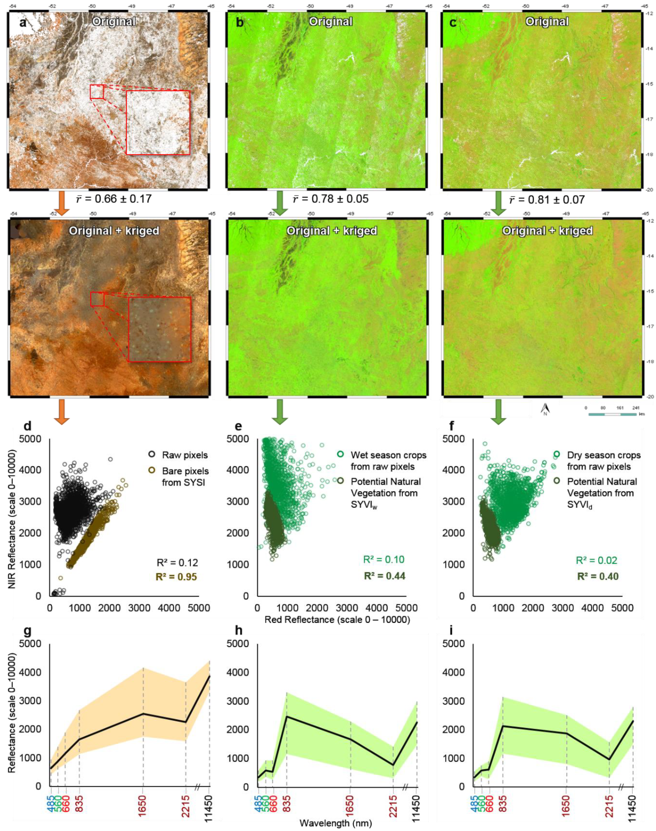
The harmonized Landsat data and the data mining algorithms implemented in GEE enabled to obtain a SySI with 443,000 km2 (52%) coverage, which was later kriged to close the gaps. The bare soil frequency (data not presented) at each locations ranged from 1 to 1303 pixels and average of 12 pixels between the 1982 and 2019 years. For potential natural vegetation from 1982 to 1994, we obtained a SyVIw with 814,175 km2 (95.2%) and a SyVId with 847,426 km2 (99.1%) coverage during the wet and dry seasons, respectively. The PNV frequency (at every locations) in the wet season ranged from 1 to 85 pixels, and mean values of 6 pixels. During the dry season, the PNV frequency had average values of 19 pixels, ranging from 1 to 185 pixels. The kriged images had satisfactory correlation (Pearson) with the originals, which presented average values of 0.66 (SySI), 0.78 (SyVIw) and 0.81 (SyVId) for the seven spectral bands (Figure 4a–c). The full coverage SySI, SyVIw and SyVId with the NA gaps interpolated by kriging (original + krikeg) were displayed in Figure 4a–c.
The soil line for bare soil (Figure 4d) had an adjustment near to the 1:1 trend line, with highly correlated values (R2 of 0.95), while raw (unprocessed) pixels extracted from a median composite (between 2017 and 2019) had a scatter distribution. For PNV, the soil line had clustered values with lower reflectance intensities (Figure 4e–f) compared to the raw pixels sampled from the median composite (between 2017 and 2019) over croplands mapped by MapBiomas [23]. The mean NIR reflectance was higher for SyVIw (2,471) than for SyVId (2,123), while the mean Red reflectance was higher for SyVId (611) than for SyVIw (536).
The spectral signature for bare soil (Figure 4g) had a constant ascendant pattern from Blue to SWIR1 regions, while the PNV (Figure 4h–i) had an opposite overall pattern, ascending from Blue to NIR and then descending to SWIR2. The SySI averaged a LST of 38.7 °C (Figure 4g), higher than for the SyVIw and SyVId, with mean values of 22.58 and 23.04 °C (Figure 4h–i), respectively.
Remaining soil covariates (Table 1) were placed in the Appendix A as Figure A1.

3.3. Model Assessments

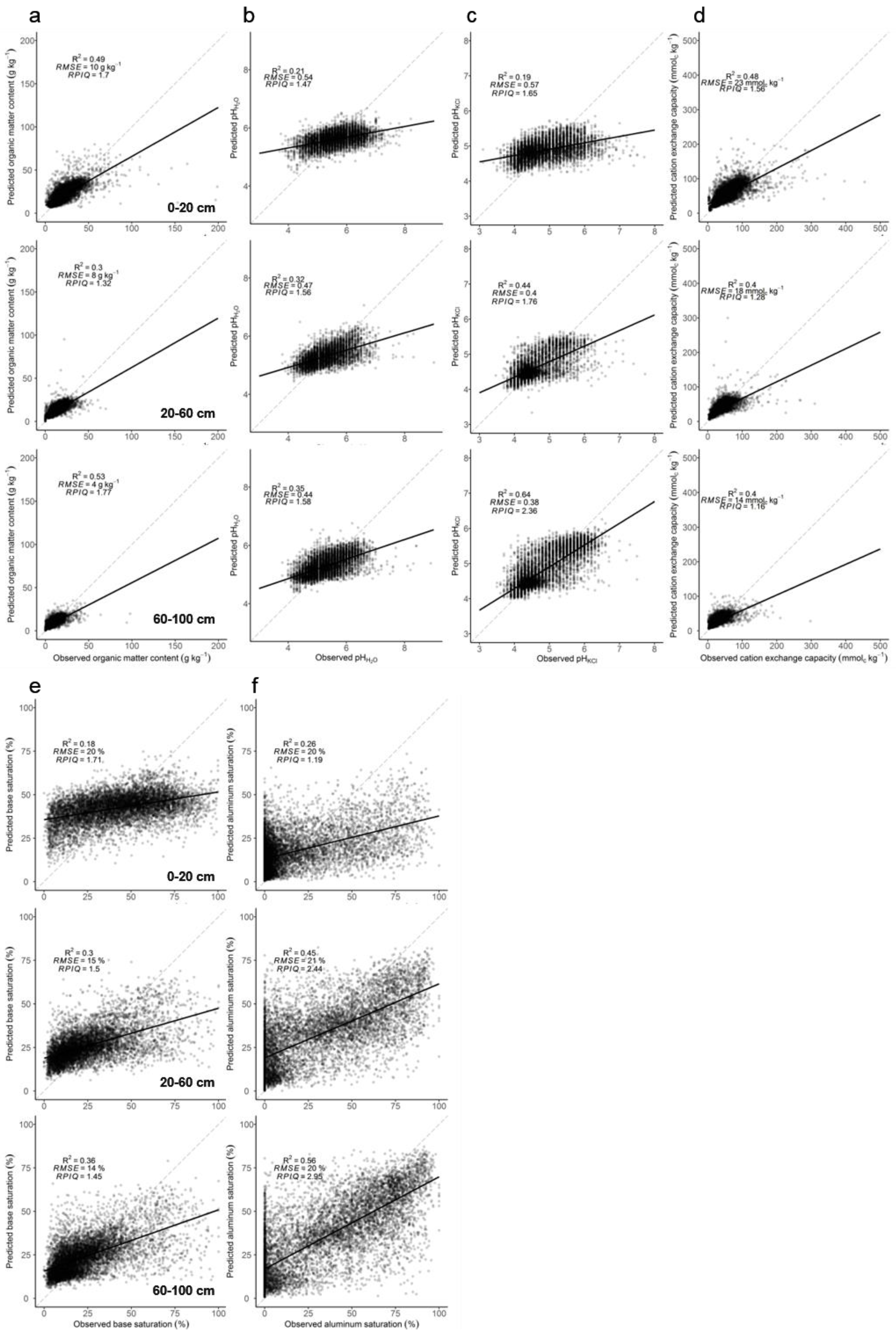
Table 3 shows the performance of optimized RF regression models on calibration (cal) and validation (10cv) sets. Predicted vs observed scatterplots from 10-fold cross-validation derived from the models of sand, silt and clay were placed in the Appendix A as Figure A2, while the remaining soil attributes are displayed in Figure A3.
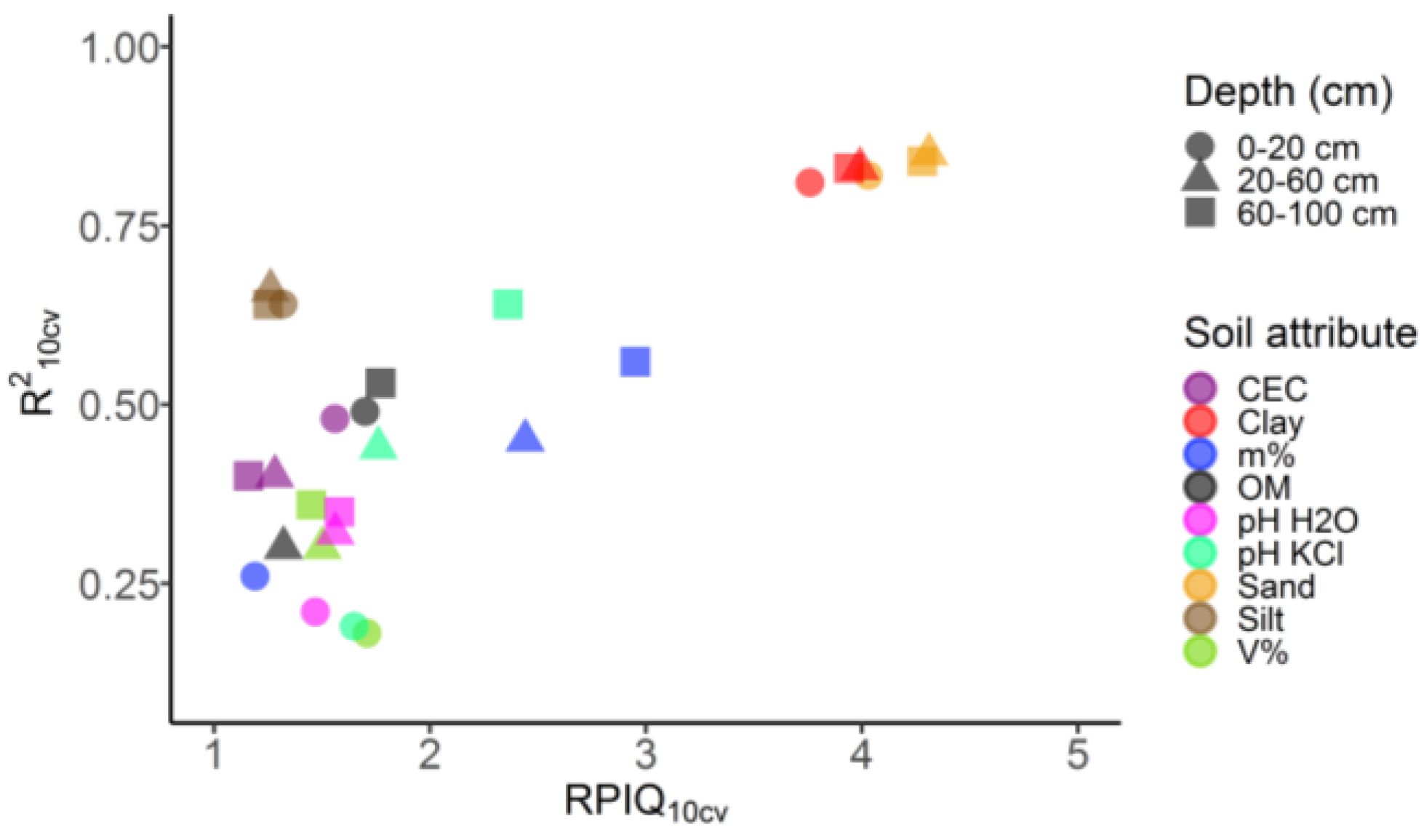
We obtained decreasing RMSE and increasing RPIQ with increasing depth interval, both in calibration and validation data. The relatively low positive values of RMSE10cv suggested that the soil variables were slightly overestimated for all the models. On average, RPIQ10cv and R210cv increased slightly from 0–20 to 60–100 cm depth, while decreased for silt and CEC. Sand and clay presented the best model’ predictive capacity with the highest RPIQ10cv (from 3.8 to 4.3), followed by m% > pH KCl > OM > V% > pH H2O > CEC > silt, ranging from 1.2 to 3.0 (Table 3).
Overall, the amount of variation explained by the spatial prediction models in validation were reasonable at all depths, with higher values for sand and clay (R210cv from 0.81 to 0.85) followed by silt (R210cv from 0.64 to 0.66). Chemical attributes were best explained for pH KCl (R210cv from 0.19 to 0.64), m% (R210cv from 0.26 to 0.56), OM (R210cv from 0.30 to 0.53) and CEC (R210cv from 0.40 to 0.48). The poorest performances were for V% (R210cv from 0.18 to 0.36) and pH H2O (R210cv from 0.21 to 0.35) (Table 3). We observed that R210cv and RPIQ10cv had a positive relationship in most models (Figure 5), where higher values indicate greater robustness in predictive capability. Models with poor performance exhibited a scatterplot (predicted vs. observed) with higher dispersion and weaker trend, while good models showed more distributed values following a stronger linear trend (Figure A2 and Figure A3).

3.4. Best Predictors

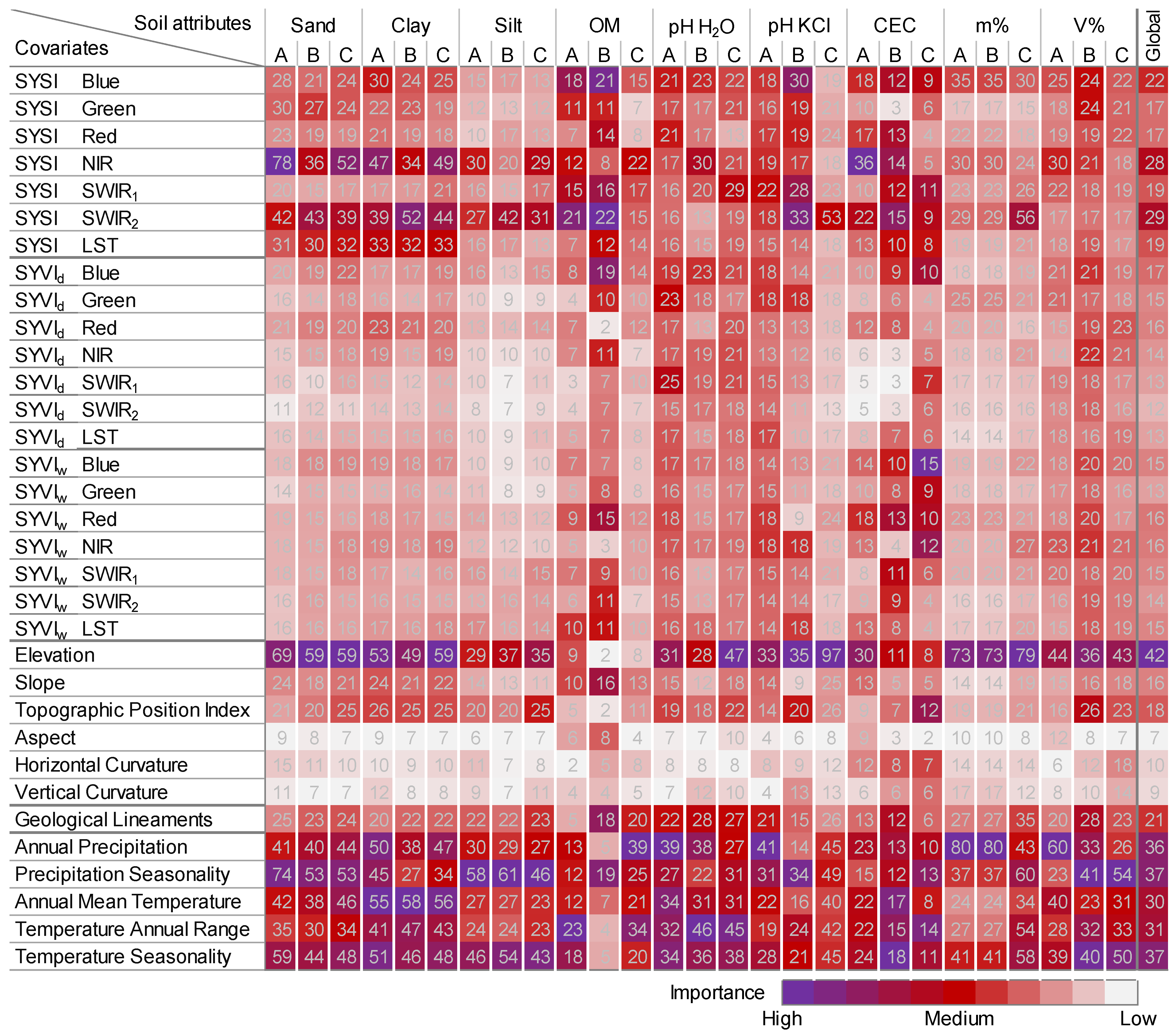
Figure 6 shows the permutation importance (%) of all the 33 covariates in RF models for the spatial prediction of 9 soil attributes at three depth intervals. From a general view (global values, Figure 6), the results indicated that the most important covariates were elevation, the five climate layers, SWIR2–NIR–Blue reflectance bands derived from SySI, ranging their estimates from 22% to 42%. The importance values did not vary much with depth, except for OM and CEC, which had slight differences. That is because the regional patterns from the coarser covariates could help the RF models in stratifying the region at the coarser level, while the more detailed information from the finer resolution covariates can represent the variability within the regional patterns.
Elevation, climate and soil reflectance derived from SYSI (NIR, SWIR2 and LST) were the most important covariates in predicting sand, clay and silt (Figure 6). In general, for predicting soil chemical attributes, climatic variables, elevation and SYSI (NIR and SWIR2 bands) seemed to be the most important, while for OM it was a combination of climatic dynamics and reflectance bands derived from SYSI, i.e., SWIR2, Blue and SWIR1.
Furthermore, the results indicated that PNV reflectance and temperature derived from SyVIw and SyVId, geological lineaments density, topographic position index and slope were mid important (from 12% to 21%) for whole soil attributes at all depths, with slightly higher values for the chemicals such as OM, pH, CEC and V% (Figure 6). In all cases, the least important were aspect, horizontal and vertical curvatures, which had an average importance of less than 10%.

3.5. Soil Maps at Multiple Depths

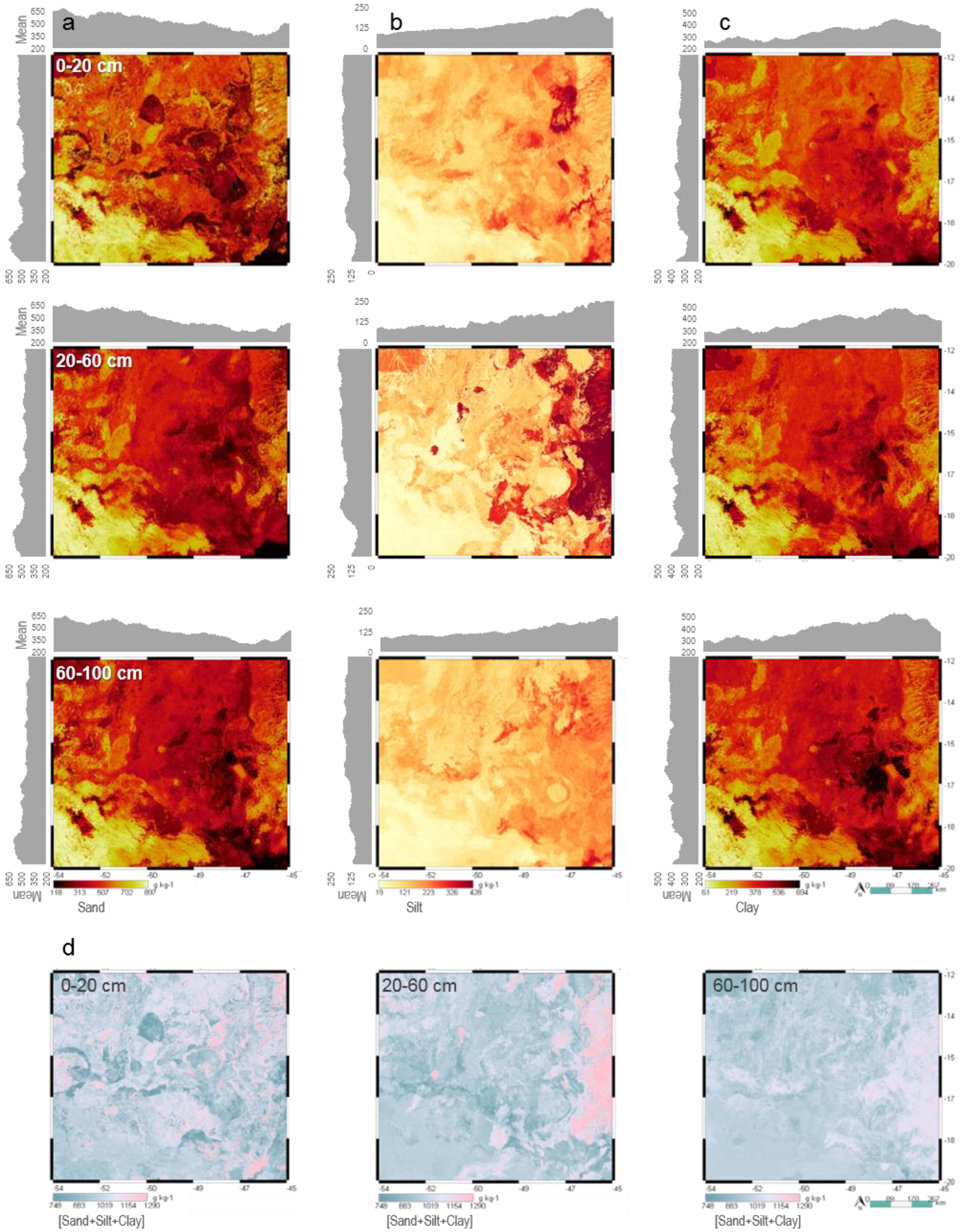
Figure 6a–c shows the maps of sand, silt and clay contents (g kg−1) in each of the three depth intervals. These maps were made publicly available for download as integer GeoTIFF format at 250 m-resolution [55]. The soils of the study region were dominated by high to moderate amounts of sand, moderate clay and little silt. Sand and clay maps were inversely distributed in the region (Figure 7a,c), due to their negative correlation (Figure 3). The largest sand contents were located southeast of the study area, decreasing gradually to the north and severely to the east. The silt and clay maps followed a very similar spatial distribution (Figure 7b,c), due to their positive correlation (Figure 3). There was more clay and silt in the east highlands of the study area, while a decreasing value was observed on the west lowlands.
In general, mean sand content decreased with depth from around 522 g kg−1 in the surface to 467 g kg−1 in the deepest layer, while at the same depths, mean clay content increased from 336 to 400 g kg−1. Average silt content remained relatively uniform with increasing depth (Figure 7).
For each depth, a map representing the sum of the sand, silt and clay contents (Figure 7d) were used to show where the estimates of soil texture diverged from 1000 g kg−1. On average, 87% of the predicted summed for the three depths ranged from 800 to 1200 g kg−1. Under and overestimates in soil texture were visually more related to the spatial patterns of the silt map (Figure 7b). Maps of the soil chemical attributes (Table 2) for all depths were placed in the Appendix A, as Figure A4.

4. Discussion

4.1. Soil Data

The soil data (BESB and FEBR) aggregated into depth intervals yielded consistent information for mapping of the selected key soil attributes (Table 2). Data showed that soil attributes and their relationship among each other were depth-dependent for different soil depth increments. In general, depth gradients in soil attributes can be assigned to the influence of soil forming factor [3]. The pedogenic processes caused different correlations among soil properties at different depths [56], thus providing differences in nutrient release for vegetation to which they may reply back with different root systems. Similar patterns were described by Goebes et al. [57], who distinguished between stable (e.g., sand, silt and clay) and dynamic (e.g., soil pH, nutrient contents, base saturation) soil attributes throughout the whole soil profile.
Despite soil observations being spatially dense and represented the main soil classes that occurs in the region (Figure 1), there are still some gaps in terms of spatial coverage. Natural vegetation and pasturelands are still under-represented. Indeed, there are many soil observations still unavailable in the region that could become open access and be used to increase spatial coverage and improve predictions [29]. Considering our large study area, we performed relatively low-cost mapping because of the use of legacy soil observations and comparatively fewer new soil observations, free RS-based covariates and the open-source R software and Google Earth Engine cloud-based platform, for data processing and visualization.

4.2. Machine Learning

RF was fairly satisfactory for DSM across the large extent of the study area (~851,000 km2), where the soil observations cannot be fully representative and the relationship between soil attributes and covariates is usually complex and non-linear [4,50]. Therefore, the regression models used covariates that captured spatial patterns from broader to more local levels across different landscapes [5]. Our validation results were similar to or even higher to those obtained in other DSMs using machine learning and cross-validation [16,17,19,21,22,34,58]. Most DSM studies recently described in literature also found tree-based models as the best option for soil spatial predictions [16,21,22]. Performance in these cases usually vary between 0.3 to 0.5 (R2), with clay content being the best predicted attribute. Variable importance indicated satellite images [16,59], elevation and climate data [16,17,60] as relevant covariates.
The good performance of the models showed that RF optimization was able to generate robust and accurate spatial predictions. This approach agreed with Probst et al. [15], who provided different optimization strategies and reported that tuning the RF hyperparameters improved the performance of regression models. Sand, silt and clay had the best performances because they are stable soil attributes, and the chemicals are dynamic along the soil profile [4]. The pH and nutrient contents may change relatively quickly (within years) related to biological processes, vegetation cover and management practices [57]. Gomes et al. [17] mapped soil organic carbon at five standard depths (from 0 to 100 cm) for Brazilian territory, where RF showed the best performance for all depths, with the highest performance at 30–60 cm for validation (R2 = 0.33). Bui et al. [60] reported similar performances for topsoil (R2 = 0.49) and subsoil (R2 = 0.36) when used analogous covariates and data mining for mapping soil organic carbon in Australia.
The better model performance in lower layers are related to soil conditions at such depths. A possible factor impacting surface-subsurface predictions are the agricultural practices, where soil management could be increasing the system’s complexity [12]. While the chemical and physical weathering are more intense and active in surface, alterations in depth tend to be less intense [59]. This suggests that the models for topsoil were more influenced by climatic variables, i.e., precipitation and temperature, which lowered the performances. Therefore, subsurface soils usually have conditions closer to the ones observed in pristine areas, and could have a better relationship with soil forming factors and covariates considered in our study.

4.3. Interpretation of Covariate Layers

We did not perform covariates selection (elimination) because this approach could generated additional load of interpretation to the project, and because RF can be used to fit models with large number of covariates [5]. For instance, Nussbaum et al. [21] evaluated six approaches for DSM of several soil variables (totaling 48 responses) using from 300–500 environmental covariates where RF models had the highest overall performances. Miller et al. [61] demonstrated that the best performing model was produced when using multi-resolution covariates, compared to a single resolution, for modeling the distribution of soil attributes at surface and subsurface. Relevant covariates for soil prediction had large importance values, whereas covariates not associated with the soil attributes showed values close to zero (Figure 6).
Our results showed that direct measurement (where soil areas are exposed) of topsoil reflectance patterns by RS was a strong contributor to soil mapping. The topsoil reflectance from SySI (Figure 4a) was important for the spatial prediction of soil attributes at the rooting depth of crops [30] in Midwest Brazil (Figure 6). That was possible because the spectral patterns of SySI can provide valuable information on pedogenic processes, which are useful for understanding and predicting soil variation [56]. The SySI also can indicate the soil weathering products, which cause spatial variations in the soil color and temporally stable soil attributes, such as mineralogy and texture [10,62]. Thus, complementary RS data can improved prediction models, as reported by Loiseau et al. [16] where adding RS covariates increased the R² and decreased the bias of the clay content estimation on bare topsoil layers (e.g., 0–30 cm).
It is recognized within the soil science community that vegetation plays significant roles on soil formation [3]. However, Savin et al. [63] stated that the use of vegetation patterns from RS for soil interpretation is insufficiently studied. Some previous works found that the spectral response of vegetation in natural conditions can be confidently used as an indirect indicator of soil attributes [64,65,66]. Our results pointed out that PNV (from SyVIw and SyVId) was influential for modelling soil attributes at all depths, especially for chemical variables (Figure 6). The soil–vegetation connection can be due to the spatial and seasonal differences in reflectance intensities between wet and dry conditions (Figure 4b–c), that showed relations between the spectral patterns of natural vegetation and soil attributes from 0 to 100 cm depth (Figure 6). Since vegetation is temporally dynamic, the relationships are largely controlled by available soil moisture and, to a lesser extent, chemical soil properties such as pH and fertility [64]. Thus, average seasonal spectral patterns of vegetation provide a better indication of soil variables than only a single snapshot of surface reflectance, and it is probably the best way to effectively represent the cumulative influence of living organisms on soil formation [4].
Climate, relief and geology played significant roles in model prediction (Figure 6) because they can significantly influence the soil-vegetation feedback, as described by [3]. The climate and geologic heterogeneity of the study region affected soil patterns at the macroscale (regional), followed by relief (especially elevation), which moderates many of the macroclimatic regimes, and landforms, at the meso and microscales [39,42]. Das Sumit [67] demonstrated that geological lineaments density was strongly related to drainage density, soil texture and soil depth, controlling the movement of groundwater through soil.
Landforms affect surface water dynamic and exposure to radiant solar energy, which directly influence soil-forming processes [42]. Within a landform, there exists slight differences in local edaphic conditions, such as soil texture and mineralogy, and soil moisture and temperature regimes [39]. These local conditions provides the most significant alterations of the soil reflectance patterns [10,62] and segregation of the plant communities [39], which could be captured and measured by the SySI, SyVIw and SyVId at the finest (local) resolution. Generally, the Keys to Soil Taxonomy [68] uses the same differing criteria to define families of soils.
Individual relationships between soil variables and environmental covariates can also be interpreted and understood in terms of pedological knowledge. For instance, higher SWIR reflectance may be associated with high amounts of sand in soil and hence lower CEC; higher precipitation and cooler temperatures frequently increase the OM content due to the speed of accumulation is higher than the speed of decomposition. For a large number of soil attributes, however, relationships are not clearly linear and often many soil covariates are equally important [4].

4.4. Reliability and Interpretation of Soil Maps

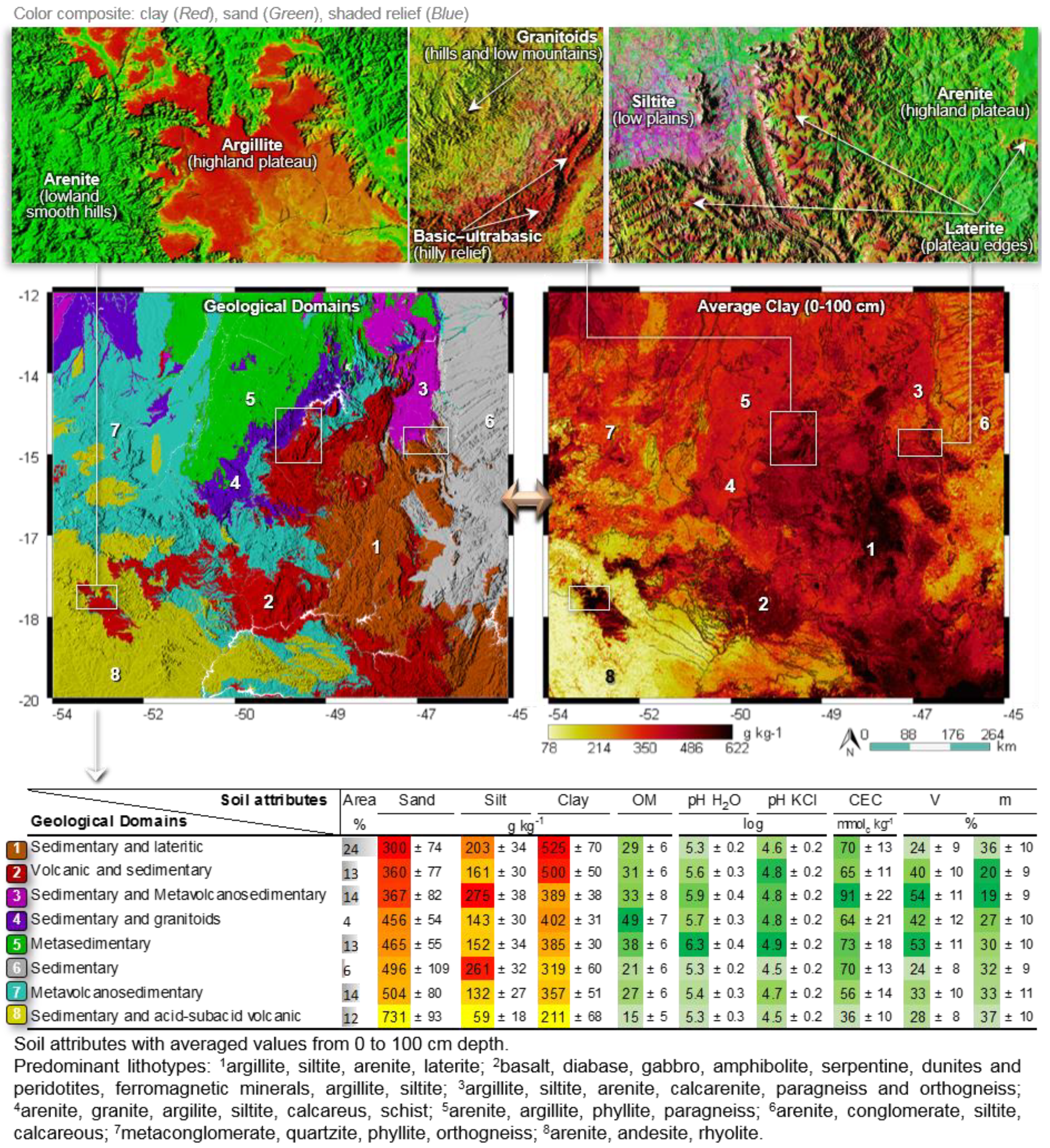
Soil attributes largely varied across the area (Figure 7 and Figure A4). This can be due to the tropical climate that exposed the parent materials of the studied soils (with different resistances) to intense weathering [69]. We identified clayey and nutrient-poor soils throughout the southeast, covering 24% of the studied area (Figure 8). The region developed upon sedimentary rocks (mostly argillite, siltite, arenite) which formed smooth hills, and over ferruginous laterite crusts supporting residual lowered plateaus in continuous dissection process [70]. The soils from these rocks (geological domain 1) had the highest clay contents with lowest chemical fertility and, in some cases, can be very acidic and contain ferruginous concretions (typically reddish color) that hinder the farming. Nevertheless, it is possible to observe several cropland areas distributed on soils of this domain [23], probably after undergoing soil chemical correction.
Clayey and medium textured soils with the best chemical conditions covered 44% of the area, widely distributed along the central portion over domains 2 to 5 (Figure 8). These domains were represented by basic-ultrabasic volcanic rocks such as basalt, diabase and gabbro, and sedimentary rocks such as argillite, siltite and calcarenite [27]. According to the geodiversity of the region [70], the areas also were constituted by an association of metamorphosed volcanic and sedimentary (metavolcanosedimentary) rocks frequently containing amphibolite, serpentine, dunites and peridotites, metacarbonates, phyllite and paragneiss. All these lithologies reworked nutrient-richer surface materials, which released nutrients into the soil and provided better fertility conditions (see domains 2 and 3 in Figure 8). Furthermore, granitoids occurred sparsely mixed with calcareous and schist (see domain 4 in Figure 8), providing more dissected relief than the neighboring lands, such as hills and low mountains that hinder the agricultural mechanization [27]. In those areas, higher elevations with denser vegetation had larger soil OM contents (Figure A1 and Figure A4), mainly due to cooler and wetter climate regimes and lesser human disturbance, which promoted accumulation processes [69]. In the floodplain areas over domain 5 (Figure 8), fertility conditions may be linked to the good fertility of the areas that surround it, from where it receives a high volume of water, sediments and wastes [70].
Sandy soils were expressive in the region, comprising 32% of the studied area (Figure 8). The lowest occurrence was in the northeast with 6% of sandy soils developed from sedimentary rocks (domain 6). They widely occurred in the southwest and midwest, developed over metavolcanosedimentary rocks (14%) and sedimentary and acid-subacid volcanic rocks (12%), domains 7 and 8 respectively. Such geological domains were mainly formed by arenite, conglomerate, siltite, calcareous, metaconglomerate, quartzite, phyllite, orthogneiss, andesite and rhyolite, which naturally tend to generate flattened reliefs such as smooth hills and plateaus [70]. These lithologies generally develop sandy soils with low chemical fertility (Figure 8). However, its high permeability and smooth reliefs facilitate agricultural mechanization after soil acidity correction and fertilization.

4.5. Possible Applications of the Maps

It is important to note that there are currently no detailed soil attribute maps with complete coverage over Midwest Brazil and that their production costs money. Our soil attribute maps can be used for different purposes, at different spatial scales from farm, local to regional. They provide a first complete assessment of key soil attributes across the Midwest region, and can be used to, for example, as input data in biological-chemical-physical modelling and in assessments of dynamic environmental processes. Together with other information, the maps can be used to obtain basic information for the implementation of colonization projects, rural subdivisions, integrated studies of micro-basins, local planning for the use and conservation of soils in areas projected for the development of agricultural, livestock and forestry projects, as well as civil engineering. The maps can also guide future soil sampling for inventory at different scales.

5. Conclusions and Final Considerations

We have demonstrated that key soil attributes from multiple depth increments can be mapped using Earth observation data and machine learning with good performances. These maps had a satisfactory performance for physical (0.64 > R210cv > 0.85) and chemical (0.18 > R210cv > 0.64) attributes at all depth intervals (0–20, 20–60 and 60–100 cm), being spatially consistent with the main lithologies from which they originated.
The methodological approach was able to capture the spatial distribution of nine soil variables. The predicted soil maps suggest that less than 44% of the studied soils had good natural fertility. Nevertheless, its dominant smooth reliefs facilitate agricultural mechanization, which allow the soil pH correction and fertilization.
Although we had representative soil observations, chemical attributes were particularly more challenging to map because to their high dynamic, with their concentration changing in a short space of time due to many natural and human-induced factors.
Our results support the notion that multi-resolution covariates derived from the topsoil and natural vegetation reflectance are important predictors of soil variability together with relief and climate data.
Since covariates widely used in digital soil mapping are globally available, such as elevation and climate data, this approach may be useful for other initiatives where obtaining the soil (SySI) and vegetation (SyVI) covariates is feasible, that is, locations around the world with bare soil and natural vegetation occurring with enough coverage within the considered satellite time series.

Author Contributions

Conceptualization, R.R.P., R.R. and J.L.S.; Methodology, R.R.P., J.L.S. and R.R.; Software, R.R.P., and J.L.S.; Validation, R.R.P.; Writing-Original Draft Preparation, R.R.P.; Writing-Review & Editing, R.R.P., R.R., J.L.S., J.A.M.D., M.P.C.L., J.J.N. and M.P.O.J.; Visualization, R.R.P.; Supervision, J.A.M.D. and M.P.C.L.

Funding

The São Paulo Research Foundation – FAPESP, grant numbers: 2014/22262-0, 2016/26124-6 and 2016/01597-9, funded this research. The Federal District Research Foundation – FAPDF, official notice 07/2015, funded the first-author’ PhD scholarship.

Acknowledgments

We thank members of the Geoprocessing and Pedomorphology Laboratory at the FAV/UnB for the fieldwork collaboration, and the Geotechnologies in Soil Science group (https://esalqgeocis.wixsite.com/english/team) for the technical support.

Conflicts of Interest

The authors declare that there is no conflict of interest related to this work.

Abbreviations

ALOSAdvanced Land Observing Satellite
DSMDigital Soil Mapping
GEEGoogle Earth Engine
OMOrganic Matter
CECCation Exchange Capacity
V%Base Saturation
m%Aluminum Saturation
SySISynthetic Soil Image
SyVIwSynthetic Vegetation Image of wet season
SyVIdSynthetic Vegetation Image of dry season
PNVPotential Natural Vegetation
IDWInverse Distance Weighted
DEMDigital Elevation Model
NIRNear infrared spectral band
SWIR1First shortwave infrared spectral band
SWIR2Second shortwave infrared spectral band
LSTLand surface temperature
RMSERoot Mean Square Error
RPIQRatio of the Performance to Inter-Quartile distance

Appendix A

Table A1 shows the specific band number of each Landsat sensor, positioned in equivalent spectral regions, which were matched into a common name (e.g., Blue, Green, Red, NIR, SWIR1, SWIR2 and LST) for an inter-sensor harmonization.
Figure A1 displays 12 of the 33 covariates used to support the spatial predictions of soil variables. These covariates were obtained using the Google Earth Engine (GEE) cloud-based platform [14], according to their possible representativeness of the soil forming factors [3]. The density of geological lineaments was obtained by counting the meters of structural lines obtained from a 1:1,000,000-scale map [27] per 1 km2.
Figure A2 and Figure A3 exhibits the predicted vs observed scatterplots of 10-fold cross-validation derived from optimized models for sand, silt and clay and the chemical attributes. The 30 m resolution maps of predicted soil chemical attributes at three distinct depth intervals are shown in the Figure A4.
Table A1. Harmonized Landsat Surface Reflectance Data Set.
Band.L4 TML5 TML7 ETM+L8 OLI/TIRS
Blue1 (450–520 nm)1 (450–520 nm)1 (450–520 nm)2 (452–512 nm)
Green2 (520–600 nm)2 (520–600 nm)2 (520–600 nm)3 (533–590 nm)
Red3 (630–690 nm)3 (630–690 nm)3 (630–690 nm)4 (636–673 nm)
NIR4 (770–900 nm)4 (770–900 nm)4 (770–900 nm)5 (851–879 nm)
SWIR15 (1550–1750 nm)5 (1550–1750 nm)5 (1550–1750 nm)6 (1566–1651 nm)
SWIR27 (2080–2350 nm)7 (2080–2350 nm)7 (2080–2350 nm)7 (2107–2294 nm)
LST6 (10,400–12,500 nm)6 (10,400–12,500 nm)6 (10,400–12,500 nm)10 (10,600–11,190 nm)
Data1982–19931984–20121999–present2013–present
L4 TM: Landsat 4 Thematic Mapper; L5 TM: Landsat 5 Thematic Mapper; L7 ETM+: Landsat 7 Enhanced Thematic Mapper Plus; L8 OLI/TIRS: Landsat 8 Operational Land Imager/Thermal Infrared Sensor; NIR: Near infrared band; SWIR1: First shortwave infrared band; SWIR2: Second shortwave infrared band; LST: Land surface temperature; Native spectral ranges are in parenthesis.
Figure A1. Environmental covariates used in the Random Forest modelling of soil attributes data. Terrain features derived from ALOS digital elevation model: (a) Elevation in meters, (b) Slope in degrees, (c) Aspect in degree, (d) Topographic Position Index, (e) Horizontal Curvature and (f) Vertical Curvature in meters. (g) Geological Lineaments Density representing meters of structural features per km2, derived from legacy maps of the Geological Survey of Brazil (CPRM). Climate data obtained from WorldClim: (h) Annual Precipitation in mm, (i) Coefficient of variation of the Precipitation Seasonality, (j) Annual Mean Temperature, (k) Temperature Annual Range and (l) Temperature Seasonality in °C.
Remotesensing 11 02905 g0a1
Figure A2. Predicted vs. observed (a) sand, (b) silt and (c) clay contents by depth intervals of 10-fold cross-validation derived from optimized random forest regression.
Remotesensing 11 02905 g0a2
Figure A3. Predicted vs. observed (a) organic matter, (b) pH H2O, (c) pH KCl, (d) cation exchange capacity, (e) base saturation and (f) aluminum saturation by depth intervals of 10-fold cross-validation derived from optimized random forest regression.
Remotesensing 11 02905 g0a3
Figure A4. Maps of (a) organic matter, (b) pH H2O, (c) pH KCl, (d) cation exchange capacity, (e) base saturation and (f) aluminum saturation predicted at three depth intervals (0–20 cm, 20–60 cm and 60–100 cm). The visualization of the images was adjusted by stretching the range of pixel values between 2% and 98%.
Remotesensing 11 02905 g0a4

References

  1. Bünemann, E.K.; Bongiorno, G.; Bai, Z.; Creamer, R.E.; De Deyn, G.; de Goede, R.; Fleskens, L.; Geissen, V.; Kuyper, T.W.; Mäder, P.; et al. Soil quality—A critical review. Soil Biol. Biochem. 2018, 120, 105–125. [Google Scholar] [CrossRef]
  2. United Nations—Department of Economic and Social Affairs—Population Division. World Population Prospects 2019: Highlights; United Nations: New York, NY, USA, 2019. Available online: https://population.un.org/wpp/Publications/Files/WPP2019_Highlights.pdf (accessed on 20 September 2019).
  3. McBratney, A.B.; Mendonça Santos, M.L.; Minasny, B. On digital soil mapping. Geoderma 2003, 117, 3–52. [Google Scholar] [CrossRef]
  4. Hengl, T.; Mendes de Jesus, J.; Heuvelink, G.B.M.; Ruiperez Gonzalez, M.; Kilibarda, M.; Blagotić, A.; Shangguan, W.; Wright, M.N.; Geng, X.; Bauer-Marschallinger, B.; et al. SoilGrids250m: Global gridded soil information based on machine learning. PLoS ONE 2017, 12, e0169748. [Google Scholar] [CrossRef] [PubMed] [Green Version]
  5. Hengl, T.; Nussbaum, M.; Wright, M.N.; Heuvelink, G.B.M.; Gräler, B. Random forest as a generic framework for predictive modeling of spatial and spatio-temporal variables. PeerJ 2018, 6, e5518. [Google Scholar] [CrossRef] [PubMed] [Green Version]
  6. Stenberg, B.; Viscarra Rossel, R.A.; Mouazen, A.M.; Wetterlind, J. Visible and Near Infrared Spectroscopy in Soil Science. Adv. Agron. 2010, 107, 163–215. [Google Scholar] [CrossRef] [Green Version]
  7. Diek, S.; Schaepman, M.E.; de Jong, R. Creating multi-temporal composites of airborne imaging spectroscopy data in support of digital soil mapping. Remote Sens. 2016, 8, 906. [Google Scholar] [CrossRef] [Green Version]
  8. Diek, S.; Fornallaz, F.; Schaepman, M.; de Jong, R. Barest Pixel Composite for Agricultural Areas Using Landsat Time Series. Remote Sens. 2017, 9, 1245. [Google Scholar] [CrossRef] [Green Version]
  9. Rogge, D.; Bauer, A.; Zeidler, J.; Mueller, A.; Esch, T.; Heiden, U. Building an exposed soil composite processor (SCMaP) for mapping spatial and temporal characteristics of soils with Landsat imagery (1984–2014). Remote Sens. Environ. 2018, 205, 1–17. [Google Scholar] [CrossRef] [Green Version]
  10. Demattê, J.A.M.; Fongaro, C.T.; Rizzo, R.; Safanelli, J.L. Geospatial Soil Sensing System (GEOS3): A powerful data mining procedure to retrieve soil spectral reflectance from satellite images. Remote Sens. Environ. 2018, 212. [Google Scholar] [CrossRef]
  11. Fongaro, C.; Demattê, J.; Rizzo, R.; Lucas Safanelli, J.; Mendes, W.; Dotto, A.; Vicente, L.; Franceschini, M.; Ustin, S. Improvement of Clay and Sand Quantification Based on a Novel Approach with a Focus on Multispectral Satellite Images. Remote Sens. 2018, 10, 1555. [Google Scholar] [CrossRef] [Green Version]
  12. Mendes, W.D.S.; Medeiros Neto, L.G.; Demattê, J.A.M.; Gallo, B.C.; Rizzo, R.; Safanelli, J.L.; Fongaro, C.T. Is it possible to map subsurface soil attributes by satellite spectral transfer models? Geoderma 2019, 343, 269–279. [Google Scholar] [CrossRef]
  13. Padarian, J.; Minasny, B.; McBratney, A.B. Machine learning and soil sciences: A review aided by machine learning tools. SOIL Discuss. 2019, 2019, 1–29. [Google Scholar] [CrossRef]
  14. Gorelick, N.; Hancher, M.; Dixon, M.; Ilyushchenko, S.; Thau, D.; Moore, R. Google Earth Engine: Planetary-scale geospatial analysis for everyone. Remote Sens. Environ. 2017, 202, 18–27. [Google Scholar] [CrossRef]
  15. Probst, P.; Wright, M.N.; Boulesteix, A.-L. Hyperparameters and tuning strategies for random forest. Wiley Interdiscip. Rev. Data Min. Knowl. Discov. 2019, 9, e1301. [Google Scholar] [CrossRef] [Green Version]
  16. Loiseau, T.; Chen, S.; Mulder, V.L.; Román Dobarco, M.; Richer-de-Forges, A.C.; Lehmann, S.; Bourennane, H.; Saby, N.P.A.; Martin, M.P.; Vaudour, E.; et al. Satellite data integration for soil clay content modelling at a national scale. Int. J. Appl. Earth Obs. Geoinf. 2019, 82, 101905. [Google Scholar] [CrossRef]
  17. Gomes, L.C.; Faria, R.M.; de Souza, E.; Veloso, G.V.; Schaefer, C.E.G.R.; Filho, E.I.F. Modelling and mapping soil organic carbon stocks in Brazil. Geoderma 2019, 340, 337–350. [Google Scholar] [CrossRef]
  18. Amirian-Chakan, A.; Minasny, B.; Taghizadeh-Mehrjardi, R.; Akbarifazli, R.; Darvishpasand, Z.; Khordehbin, S. Some practical aspects of predicting texture data in digital soil mapping. Soil Tillage Res. 2019, 194, 104289. [Google Scholar] [CrossRef]
  19. Ma, Y.; Minasny, B.; Wu, C. Mapping key soil properties to support agricultural production in Eastern China. Geoderma Reg. 2017, 10, 144–153. [Google Scholar] [CrossRef]
  20. Keskin, H.; Grunwald, S.; Harris, W.G. Digital mapping of soil carbon fractions with machine learning. Geoderma 2019, 339, 40–58. [Google Scholar] [CrossRef]
  21. Nussbaum, M.; Spiess, K.; Baltensweiler, A.; Grob, U.; Keller, A.; Greiner, L.; Schaepman, M.E.; Papritz, A. Evaluation of digital soil mapping approaches with large sets of environmental covariates. SOIL 2018, 4, 1–22. [Google Scholar] [CrossRef] [Green Version]
  22. Hengl, T.; Heuvelink, G.B.M.; Kempen, B.; Leenaars, J.G.B.; Walsh, M.G.; Shepherd, K.D.; Sila, A.; MacMillan, R.A.; Mendes de Jesus, J.; Tamene, L.; et al. Mapping Soil Properties of Africa at 250 m Resolution: Random Forests Significantly Improve Current Predictions. PLoS ONE 2015, 10, e0125814. [Google Scholar] [CrossRef] [PubMed]
  23. Parente, L.; Mesquita, V.; Miziara, F.; Baumann, L.; Ferreira, L. Assessing the pasturelands and livestock dynamics in Brazil, from 1985 to 2017: A novel approach based on high spatial resolution imagery and Google Earth Engine cloud computing. Remote Sens. Environ. 2019, 232, 111301. [Google Scholar] [CrossRef]
  24. IBGE—Instituto Brasileiro de Geografia e Estatística Produção Agrícola Municipal [Municipal Agricultural Production]. Available online: https://sidra.ibge.gov.br/pesquisa/pam/tabelas (accessed on 29 September 2019).
  25. IBGE—Instituto Brasileiro de Geografia e Estatística Pedologia [Pedological maps of Brazil]. Available online: https://www.ibge.gov.br/geociencias/informacoes-ambientais/pedologia/10871-pedologia.html?=&t=downloads (accessed on 30 September 2019).
  26. IUSS Working Group WRB. World Reference Base for Soil Resources 2014: International Soil Classification System for Naming Soils and Creating Legends for Soil Maps; Food and Agriculture Organization: Rome, Italy, 2015; Available online: http://www.fao.org/3/i3794en/I3794EN.pdf (accessed on 01 September 2019).
  27. CPRM—Companhia de Pesquisa de Recursos Minerais. Carta Geológica do Brasil ao Milionésimo: Sistema de Informações Geográficas-SIG [Geological Map of Brazil 1:1.000.000 Scale: Geographic Information System-GIS]; CPRM: Brasília, Brazil, 2004. Available online: http://www.cprm.gov.br/publique/Geologia/Geologia-Basica/Carta-Geologica-do-Brasil-ao-Milionesimo-298.html (accessed on 02 September 2019).
  28. Demattê, J.A.M.; Dotto, A.C.; Paiva, A.F.S.; Sato, M.V.; Dalmolin, R.S.D.; Araújo, M.S.B.; Silva, E.B.; Nanni, M.R.; ten Caten, A.; Noronha, N.C.; et al. The Brazilian Soil Spectral Library (BSSL): A general view, application and challenges. Geoderma 2019, 354, 113793. [Google Scholar] [CrossRef]
  29. Samuel-Rosa, A.; Dalmolin, R.S.D.; Moura-Bueno, J.M.; Teixeira, W.G.; Alba, J.M.F. Open legacy soil survey data in Brazil: Geospatial data quality and how to improve it. Sci. Agric. 2017, 77, e20170430. [Google Scholar] [CrossRef]
  30. Canadell, J.; Jackson, R.B.; Ehleringer, J.B.; Mooney, H.A.; Sala, O.E.; Schulze, E.-D. Maximum rooting depth of vegetation types at the global scale. Oecologia 1996, 108, 583–595. [Google Scholar] [CrossRef]
  31. Embrapa—Brazilian Agricultural Research Corporation—National Soils Research Center. Manual of Soil Analysis Methods, 3rd ed.; Teixeira, P.C., Donagemma, G.K., Fontana, A., Teixeira, W.G., Eds.; Embrapa Solos: Brasilia, DF, USA, 2017; Available online: http://ainfo.cnptia.embrapa.br/digital/bitstream/item/171907/1/Manual-de-Metodos-de-Analise-de-Solo-2017.pdf (accessed on 15 September 2019).
  32. Gu, Z. Circlize: Circular Visualization. 2019. Available online: https://cran.r-project.org/web/packages/circlize/index.html (accessed on 15 September 2019).
  33. R Core Team. R: A Language and Environment for Statistical Computing; R Foundation for Statistical Computing: Vienna, Austria, 2018; Available online: https://www.r-project.org/ (accessed on 15 September 2019).
  34. Viscarra Rossel, R.A.; Chen, C.; Grundy, M.J.; Searle, R.; Clifford, D.; Campbell, P.H. The Australian three-dimensional soil grid: Australia’s contribution to the GlobalSoilMap project. Soil Res. 2015, 53, 845–864. [Google Scholar] [CrossRef] [Green Version]
  35. Hengl, T.; de Jesus, J.M.; MacMillan, R.A.; Batjes, N.H.; Heuvelink, G.B.M.; Ribeiro, E.; Samuel-Rosa, A.; Kempen, B.; Leenaars, J.G.B.; Walsh, M.G.; et al. SoilGrids1km—Global Soil Information Based on Automated Mapping. PLoS ONE 2014, 9, e105992. [Google Scholar] [CrossRef] [Green Version]
  36. Liang, Z.; Chen, S.; Yang, Y.; Zhou, Y.; Shi, Z. High-resolution three-dimensional mapping of soil organic carbon in China: Effects of SoilGrids products on national modeling. Sci. Total Environ. 2019, 685, 480–489. [Google Scholar] [CrossRef]
  37. Ballabio, C.; Lugato, E.; Fernández-Ugalde, O.; Orgiazzi, A.; Jones, A.; Borrelli, P.; Montanarella, L.; Panagos, P. Mapping LUCAS topsoil chemical properties at European scale using Gaussian process regression. Geoderma 2019, 355, 113912. [Google Scholar] [CrossRef]
  38. Akinyemi, F.; Adejuwon, J. A GIS-Based Procedure for Downscaling Climate Data for West Africa. Trans. GIS 2008, 12, 613–631. [Google Scholar] [CrossRef]
  39. Bailey, R.G. Suggested hierarchy of criteria for multi-scale ecosystem mapping. Landsc. Urban Plan. 1987, 14, 313–319. [Google Scholar] [CrossRef] [Green Version]
  40. Hijmans, R.J.; Cameron, S.E.; Parra, J.L.; Jones, P.G.; Jarvis, A. Very high resolution interpolated climate surfaces for global land areas. Int. J. Climatol. 2005, 25, 1965–1978. [Google Scholar] [CrossRef]
  41. Tadono, T.; Ishida, H.; Oda, F.; Naito, S.; Minakawa, K.; Iwamoto, H. Precise global DEM generation by ALOS PRISM. ISPRS Ann. Photogramm. Remote Sens. Spat. Inf. Sci. 2014, II-4, 71–76. [Google Scholar] [CrossRef] [Green Version]
  42. Florinsky, I.V. Digital Terrain Analysis in Soil Science and Geology; Academic press: Sydney, Australia, 2016. [Google Scholar] [CrossRef]
  43. USGS—United States Geological Survey. Landsat 4–7 Surface Reflectance Code LEDAPS Product Guide; Department of the Interior, USGS: Lawrence, KS, USA, 2019. Available online: https://www.usgs.gov/media/files/landsat-4-7-surface-reflectance-code-ledaps-product-guide (accessed on 17 September 2019).
  44. USGS—United States Geological Survey. Landsat 8 Surface Reflectance Code LaSRC Product Guide; Department of the Interior, USGS: Lawrence, KS, USA, 2019. Available online: https://www.usgs.gov/media/files/land-surface-reflectance-code-lasrc-product-guide (accessed on 17 September 2019).
  45. Vandegriend, A.; Owe, M.; Vugts, H.; Ramothwa, G. Botswana Water and Surface Energy Balance Research Program. Part 1: Integrated Approach and Field Campaign Results; NASA Goddard Space Flight Center: Greenbelt, MD, USA, 1992. Available online: https://ntrs.nasa.gov/search.jsp?R=19930011702 (accessed on 18 September 2019).
  46. Al-Gaadi, K.A.; Hassaballa, A.A.; Tola, E.; Kayad, A.G.; Madugundu, R.; Assiri, F.; Alblewi, B. Characterization of the spatial variability of surface topography and moisture content and its influence on potato crop yield. Int. J. Remote Sens. 2018, 39, 8572–8590. [Google Scholar] [CrossRef]
  47. Gallo, B.; Demattê, J.; Rizzo, R.; Safanelli, J.; Mendes, W.; Lepsch, I.; Sato, M.; Romero, D.; Lacerda, M. Multi-Temporal Satellite Images on Topsoil Attribute Quantification and the Relationship with Soil Classes and Geology. Remote Sens. 2018, 10, 1571. [Google Scholar] [CrossRef]
  48. McBratney, A.B.; Webster, R. Choosing functions for semi-variograms of soil properties and fitting them to sampling estimates. J. Soil Sci. 1986, 37, 617–639. [Google Scholar] [CrossRef]
  49. Baret, F.; Jacquemoud, S.; Hanocq, J.F. About the soil line concept in remote sensing. Adv. Space Res. 1993, 13, 281–284. [Google Scholar] [CrossRef]
  50. Breiman, L. Random forests. Mach. Learn. 2001, 45, 5–32. [Google Scholar] [CrossRef] [Green Version]
  51. FAO. Soil Organic Carbon Mapping Cookbook, 2nd ed.; FAO: Rome, Italy, 2018; Available online: http://www.fao.org/documents/card/en/c/I8895EN (accessed on 20 September 2019).
  52. Wright, M.N.; Ziegler, A. Ranger: A Fast Implementation of Random Forests for High Dimensional Data in C++ and R. arXiv 2017, arXiv:1508.04409. [Google Scholar] [CrossRef] [Green Version]
  53. Kuhn, M. Caret: Classification and Regression Training. 2019. Available online: https://cran.r-project.org/web/packages/caret/index.html (accessed on 21 September 2019).
  54. Bellon-Maurel, V.; Fernandez-Ahumada, E.; Palagos, B.; Roger, J.-M.; McBratney, A. Critical review of chemometric indicators commonly used for assessing the quality of the prediction of soil attributes by NIR spectroscopy. TrAC Trends Anal. Chem. 2010, 29, 1073–1081. [Google Scholar] [CrossRef]
  55. Poppiel, R.R.; Lacerda, M.P.C.; Safanelli, J.L.; Rizzo, R.; Oliveira, M.P., Jr.; Novais, J.J.; Demattê, J.A.M. 250 m-gridded soil texture at multiple depths of Midwest Brazil. Data Mendeley 2019. [Google Scholar] [CrossRef]
  56. Ma, Y.; Minasny, B.; Malone, B.P.; Mcbratney, A.B. Pedology and digital soil mapping (DSM). Eur. J. Soil Sci. 2019, 70, 216–235. [Google Scholar] [CrossRef]
  57. Goebes, P.; Schmidt, K.; Seitz, S.; Both, S.; Bruelheide, H.; Erfmeier, A.; Scholten, T.; Kühn, P. The strength of soil-plant interactions under forest is related to a Critical Soil Depth. Sci. Rep. 2019, 9, 8635. [Google Scholar] [CrossRef] [PubMed] [Green Version]
  58. Vaudour, E.; Gomez, C.; Fouad, Y.; Lagacherie, P. Sentinel-2 image capacities to predict common topsoil properties of temperate and Mediterranean agroecosystems. Remote Sens. Environ. 2019, 223, 21–33. [Google Scholar] [CrossRef]
  59. Bui, E.N.; Henderson, B.L.; Viergever, K. Knowledge discovery from models of soil properties developed through data mining. Ecol. Model. 2006, 191, 431–446. [Google Scholar] [CrossRef]
  60. Bui, E.; Henderson, B.; Viergever, K. Using knowledge discovery with data mining from the Australian Soil Resource Information System database to inform soil carbon mapping in Australia. Global Biogeochem. Cycles 2009, 23. [Google Scholar] [CrossRef]
  61. Miller, B.A.; Koszinski, S.; Wehrhan, M.; Sommer, M. Impact of multi-scale predictor selection for modeling soil properties. Geoderma 2015, 239, 97–106. [Google Scholar] [CrossRef]
  62. Poppiel, R.R.; Lacerda, M.P.C.; Demattê, J.A.M.; Oliveira, M.P., Jr.; Gallo, B.C.; Safanelli, J.L. Pedology and soil class mapping from proximal and remote sensed data. Geoderma 2019, 348, 189–206. [Google Scholar] [CrossRef]
  63. Savin, I.Y.; Zhogolev, A.V.; Prudnikova, E.Y. Modern Trends and Problems of Soil Mapping. Eurasian Soil Sci. 2019, 52, 471–480. [Google Scholar] [CrossRef]
  64. Maynard, J.J.; Levi, M.R. Hyper-temporal remote sensing for digital soil mapping: Characterizing soil-vegetation response to climatic variability. Geoderma 2017, 285, 94–109. [Google Scholar] [CrossRef] [Green Version]
  65. Serteser, A.; Kargιoğlu, M.; Içağa, Y.; Konuk, M. Vegetation as an Indicator of Soil Properties and Water Quality in the Akarçay Stream (Turkey). Environ. Manag. 2008, 42, 764. [Google Scholar] [CrossRef] [PubMed]
  66. Hengl, T.; Walsh, M.G.; Sanderman, J.; Wheeler, I.; Harrison, S.P.; Prentice, I.C. Global mapping of potential natural vegetation: An assessment of machine learning algorithms for estimating land potential. PeerJ 2018, 6, e5457. [Google Scholar] [CrossRef] [PubMed] [Green Version]
  67. Das, S. Comparison among influencing factor, frequency ratio, and analytical hierarchy process techniques for groundwater potential zonation in Vaitarna basin, Maharashtra, India. Groundw. Sustain. Dev. 2019, 8, 617–629. [Google Scholar] [CrossRef]
  68. Soil Survey Staff. Keys to Soil Taxonomy; United States Department of Agriculture: Washington, DC, USA, 2014; Volume 12. Available online: http://www.nrcs.usda.gov/Internet/FSE_DOCUMENTS/nrcs142p2_051546.pdf (accessed on 22 September 2019).
  69. Vieira, B.C.; Salgado, A.A.R.; Santos, L.J.C. Landscapes and Landforms of Brazil; Springer: Berlin/Heidelberg, Germany, 2015; Available online: https://link.springer.com/book/10.1007%2F978-94-017-8023-0#editorsandaffiliations (accessed on 22 September 2019).
  70. Moraes, J.M. Geodiversidade do Estado de Goiás e do Distrito Federal [Geodiversity of Goiás State and the Federal District, Brazil]; CPRM: Goiânia, GO, USA, 2014. Available online: http://rigeo.cprm.gov.br/jspui/handle/doc/16732 (accessed on 21 September 2019).
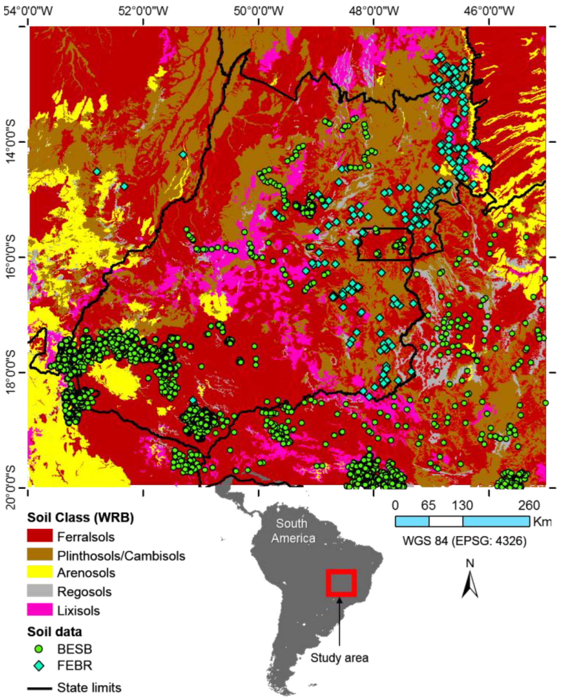
Figure 1. Spatial distribution of soil observations displayed over a 1:1,000,000-scale map of the main soil classes of the study area [25]. Soil classes were defined according to World Reference Base [26].
Remotesensing 11 02905 g001
Figure 2. Digital soil mapping framework used for generating soil attribute maps.
Remotesensing 11 02905 g002
Figure 3. Chord diagram based on Pearson correlation (r) among all measured soil attributes at (a) 0–20 cm, (b) 20–60 cm and (c) 60–100 cm depth intervals; and (d) overall correlation with depth intervals. Blue and red colors symbolize positive and negative correlations, respectively.
Remotesensing 11 02905 g003
Figure 4. Soil covariates obtained by data mining and statistics of Landsat data. (a) SySI (RGB: Red, Green, Blue), (b) SyVIw and (c) SyVId (RGB: SWIR1, NIR, Red) subsets. Soil line charts for (d) SySI vs raw pixels, (e) SyVIw vs wet season crops obtained from raw pixels and (f) SyVId vs dry season crops obtained from raw pixels. Minimum, average and maximum spectra collected from (g) SySI, (h) SyVIw and (i) SyVId. The visualization of the images was adjusted by stretching the range of pixel values between 2% and 98%. Optical bands are positioned in the mean spectral range from 485 to 2215 nm, and the thermal band at 11,450 nm. r ¯ : average of Pearson’s correlation from the seven spectral bands, performed by sampling 1 value km−2 on overlapped areas between the synthetic image (original) and kriged (non-merged to synthetic image).
Remotesensing 11 02905 g004
Figure 5. Performance indicators of optimized models used in the soil predictions by depth interval.
Remotesensing 11 02905 g005
Figure 6. Permutation importance (%) of covariates for prediction soil attributes at 0–20 cm (A), 20–60 cm (B) and 60–100 cm (B) depth intervals. The mean values were calculated from the importance obtained by the 10-fold used in cross-validation. CEC: cation exchange capacity; m%: Aluminum saturation; V%: Base saturation. Global represents averaged importance values for all soil attributes.
Remotesensing 11 02905 g006
Figure 7. Maps and mean lat/long distribution chart of (a) sand, (b) silt and (c) clay content (g kg−1) for different depth intervals (0–20 cm, 20–60 cm and 60–100 cm). The sum of the sand, silt and clay contents [Sand+Silt+Clay] for each depth interval appears in (d). The visualization of the images was adjusted by stretching the range of pixel values between 2% and 98%.
Remotesensing 11 02905 g007
Figure 8. Geological domains and summary values of predicted soil attributes averaged from the three depth intervals. The geological domains were obtained by clustering lithologies using the averaged soil data. The main lithotypes were identified within each domain according the geological map [27].
Remotesensing 11 02905 g008
Table 1. List of Covariates used for Digital Mapping of Soil Attributes.
CovariateDescriptionNative Scale
or Resolution
Source
Soil, Parent Material and Age
Synthetic Soil Image (SySI)Bare soil reflectance covering
VNIR-SWIR-TIR range (7 bands)
30 mLandsat 4, 5, 7 and 8
Geological Lineaments DensityMeters of structural features per km21:1,000,000 aCPRM
Organisms
Synthetic Vegetation Image
of dry season (SyVId)
Potential natural vegetation reflectance from November to March covering VNIR-SWIR-TIR range (7 bands)30 mLandsat 4 and 5
Synthetic Vegetation Image
of wet season (SyVIw)
Potential natural vegetation reflectance from May to September covering VNIR-SWIR-TIR range (7 bands)30 mLandsat 4 and 5
Climate
Annual Precipitation (mm)Bioclimatic variables obtained from the monthly temperature and rainfall in order to generate more biologically meaningful values.1 km bWorldClim
Precipitation Seasonality (CV)1 km bWorldClim
Annual Mean Temperature (°C)1 km bWorldClim
Temperature Annual Range (°C)1 km bWorldClim
Temperature Seasonality (°C)1 km bWorldClim
Relief and Age
Elevation (m)Height of terrain above sea level30 mALOS
Slope (degree)Slope gradient30 mALOS
Aspect (degree)Compass direction30 mALOS
Topographic Position Index (m)Distinguishes ridge from valley forms30 mALOS
Horizontal Curvature (m)Curvature tangent to the contour line30 mALOS
Vertical Curvature (m)Curvature tangent to the slope line30 mALOS
VNIR: Visible and Near infrared spectral range (~450–900 nm); SWIR: Shortwave infrared spectral range (~1550–2350 nm); TIR: Thermal infrared spectral range (~10,400–12,500 nm). a Lines counted in grids of 1 km2, transformed to raster and interpolated to 30 m pixel resolution by IDW method. b Interpolated to 30 m pixel resolution by Inverse Distance Weighted method; CV: coefficient of variation.
Table 2. Statistical Summary of Soil Data Aggregated into Different Depth Intervals for Spatial Modelling.
Soil AttributeDepth (cm)nMin.Q1MeanMedianQ3Max.SdIQRSkew.
Clay (g kg−1)0–20793010872711764509202213630.8
20–606908101002871764829302333820.8
60–1007520121253142255009502313750.8
Silt (g kg−1)0–20793012477389481689702.3
20–60690712471378276079582.3
60–100752012467378079475562.6
Sand (g kg−1)0–2079301409652783883975280474-0.8
20–6069071393643783873973284480-0.8
60–10075201377619741848967276471-0.7
Organic Matter (g kg−1)0–20724201121172839314174.8
20–6060210713111741291015.2
60–100680804981298672.3
pH H2O (log)0–2062003.75.25.65.66.08.20.60.80.1
20–6051493.84.95.35.25.69.00.60.70.7
60–10075113.84.95.35.25.69.10.50.70.7
pH KCl (log)0–2055963.14.64.94.85.37.70.61.00.6
20–6047070.44.24.64.44.97.70.50.71.1
60–10073843.54.34.84.55.27.50.60.90.9
CEC (mmolc kg−1)0–20801023253456864133373.0
20–60685222236324569623235.7
60–100765511626223258218166.2
Base Saturation (V%)0–20801802442425810022340.2
20–60686001225213410018231.2
60–100765501023183110017201.5
Aluminum Saturation (m%)0–207964001642410023241.6
20–6068410533285710029520.4
60–10076350336346210030590.3
n: number of soil observations; Min.: minimum value; Q1/Q3: 1st (25%) and 3rd (75%) quartiles; Max.: maximum value; Sd: standard deviation; IQR: interquartile range; Skew: skewness; Organic Matter = o r g a n i c   c a r b o n   × 1.72 ; CEC: cation   exchange   capacity = ( C a 2 + + M g 2 + + K + + H + + A l 3 + ) ; ( V % = ( ( C a 2 + + M g 2 + + K + ) × 100 ) ÷ C E C ); m % = ( ( A l 3 + × 100 ) ÷ ( C a 2 + + M g 2 + + K + + A l 3 + ) ) .
Table 3. Hyperparameters and Performance of the Optimized Models used for Spatial Predictions of Continuous Soil Attributes at Distinct Depth Intervals.
Soil AttributeDepth (cm)mTryminNSRMSEcalRPIQcalR2calRMSE10cvRPIQ10cvR210cv
Clay (g kg−1)0–20245399.40.97963.80.81
20–602453810.00.97964.00.83
60–100245389.90.97954.00.83
Silt (g kg−1)0–20245213.30.94531.30.64
20–60335183.20.95461.30.66
60–100245183.10.94451.30.64
Sand (g kg−1)0–203354710.10.971184.00.82
20–602454510.70.981114.30.85
60–1002454410.60.971104.30.84
Organic Matter (g kg−1)0–2033544.10.91101.70.49
20–6033533.40.9081.30.30
60–10024524.30.9241.80.53
pH H2O (log)0–203350.213.70.880.541.50.21
20–603350.193.90.890.471.60.32
60–1003350.183.90.900.441.60.35
pH KCl (log)0–203350.234.20.870.571.70.19
20–603350.164.30.910.401.80.44
60–1002450.155.90.940.382.40.64
CEC (mmolc kg−1)0–20335103.70.91231.60.48
20–6024583.00.89181.30.40
60–10024562.70.89141.20.40
Base Saturation (V%)0–2033584.40.87201.70.18
20–6033563.70.89151.50.30
60–10033563.60.89141.50.36
Aluminum Saturation (m%)0–2033582.90.88201.20.26
20–6033596.10.91212.40.45
60–10024587.40.93203.00.56
CEC: Cation exchange capacity; mTry: hyperparameter that regulates the number of variables that can be randomly sampled in each split of the trees; minNS: minimum node size, a hyperparameter that controls the tree depth by setting the minimal number of samples for the terminal nodes. RMSEcal: Root Mean Square Error of calibration; RMSE10cv: Root Mean Square Error of 10-fold cross-validation; RPIQcal: Ratio of the Performance to Inter-Quartile distance of calibration; RPIQ10cv: Ratio of the Performance to Inter-Quartile distance of 10-fold cross-validation; R2cal: Coefficient of determination of calibration; R210cv: Coefficient of determination of 10-fold cross-validation.