Assessment of the Degree of Building Damage Caused by Disaster Using Convolutional Neural Networks in Combination with Ordinal Regression

Abstract

We propose a new convolutional neural networks method in combination with ordinal regression aiming at assessing the degree of building damage caused by earthquakes with aerial imagery. The ordinal regression model and a deep learning algorithm are incorporated to make full use of the information to improve the accuracy of the assessment. A new loss function was introduced in this paper to combine convolutional neural networks and ordinal regression. Assessing the level of damage to buildings can be considered as equivalent to predicting the ordered labels of buildings to be assessed. In the existing research, the problem has usually been simplified as a problem of pure classification to be further studied and discussed, which ignores the ordinal relationship between different levels of damage, resulting in a waste of information. Data accumulated throughout history are used to build network models for assessing the level of damage, and models for assessing levels of damage to buildings based on deep learning are described in detail, including model construction, implementation methods, and the selection of hyperparameters, and verification is conducted by experiments. When categorizing the damage to buildings into four types, we apply the method proposed in this paper to aerial images acquired from the 2014 Ludian earthquake and achieve an overall accuracy of 77.39%; when categorizing damage to buildings into two types, the overall accuracy of the model is 93.95%, exceeding such values in similar types of theories and methods.

1. Introduction

The rapid and accurate acquisition of disaster losses can provide great help for disaster emergency response and decision-making. Remote sensing (RS) and Geographic Information System (GIS) can help assess earthquake damage within a short period of time after the event.

Many studies have presented assessment techniques for earthquake building damage by using aerial or satellite images [1,2,3,4,5]. Booth et al. [6] used vertical aerial images, Pictometry images, and ground observations to assess building damage in the 2011 Haitian earthquake. Building by building visual damage interpretation [7] based on the European Macroseismic Scale (EMS-98) [8] was carried out in a case study of the Bam earthquake. Huyck et al. [9] used multisensor optical satellite imagery to map citywide damage with neighborhood edge dissimilarities. Many different features have been introduced to determine building damage from remote sensing images [10]. Anniballe et al. [11] investigated the capability of earthquake damage mapping at the scale of individual buildings with a set of 13 change detention features and support vector machine (SVM). Simon Plank [12] reviewed the methods of rapid damage assessment using multitemporal Synthetic Aperture Radar(SAR) data. Gupta et al. [13] present a satellite imagery dataset for building damage assessment with over 700,000 labeled building instances covering over 5000 km² of imagery.

Recent studies show that the machine learning algorithm performs well in earthquake damage assessment. Li [14] assessed building damage with one-class SVM using pre- and post-earthquake QuickBird imagery and assessed the discrimination power of different level (pixel-level, texture, and object-based) features. Haiyang et al. [15] combined SVM and the image segmentation method to detect building damage. Cooner et al. [16] evaluate the effectiveness of machine learning algorithms in detecting earthquake damage. A series of textural and structural features were used in this study. A SVM and feature selection approach was carried out for damage mapping with post-event very high spatial resolution(VHR) image and obtained overall accuracy (OA) of 96.8% and Kappa of 0.5240 [11]. Convolutional neural networks (CNN) was utilized to identify collapsed buildings from post-event satellite imagery and obtained an OA of 80.1% and Kappa of 0.46 [17]. Multiresolution feature maps were derived and fused with CNN for the image classification of building damages in [18], and an OA of 88.7% was obtained.

Most of the above-mentioned damage information extraction studies classified damaged buildings into two classes: damaged and intact. However, these two classes are not enough to meet actual needs.

Recently, deep learning (DL) methods have provided new ideas for remote sensing image recognition technology. An end-to-end framework with CNN for satellite image classification was proposed in [19]. Scott et al. [20] used transfer learning and data augmentation to demonstrate the performance of CNNs for remote sensing land-cover classification. Zou et al. [21] proposed a DL method for remote sensing scene classification. A DL-based image classification framework was introduced in [22]. Xie et al. [23] designed a deep CNN model that can achieve a multilevel detection of clouds. Chen et al. [24] combined a pretrained CNN feature extractor and the k-Nearest Neighbor(KNN) method to improve the performance of ship classification from remote sensing images.

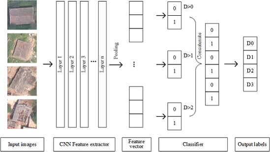
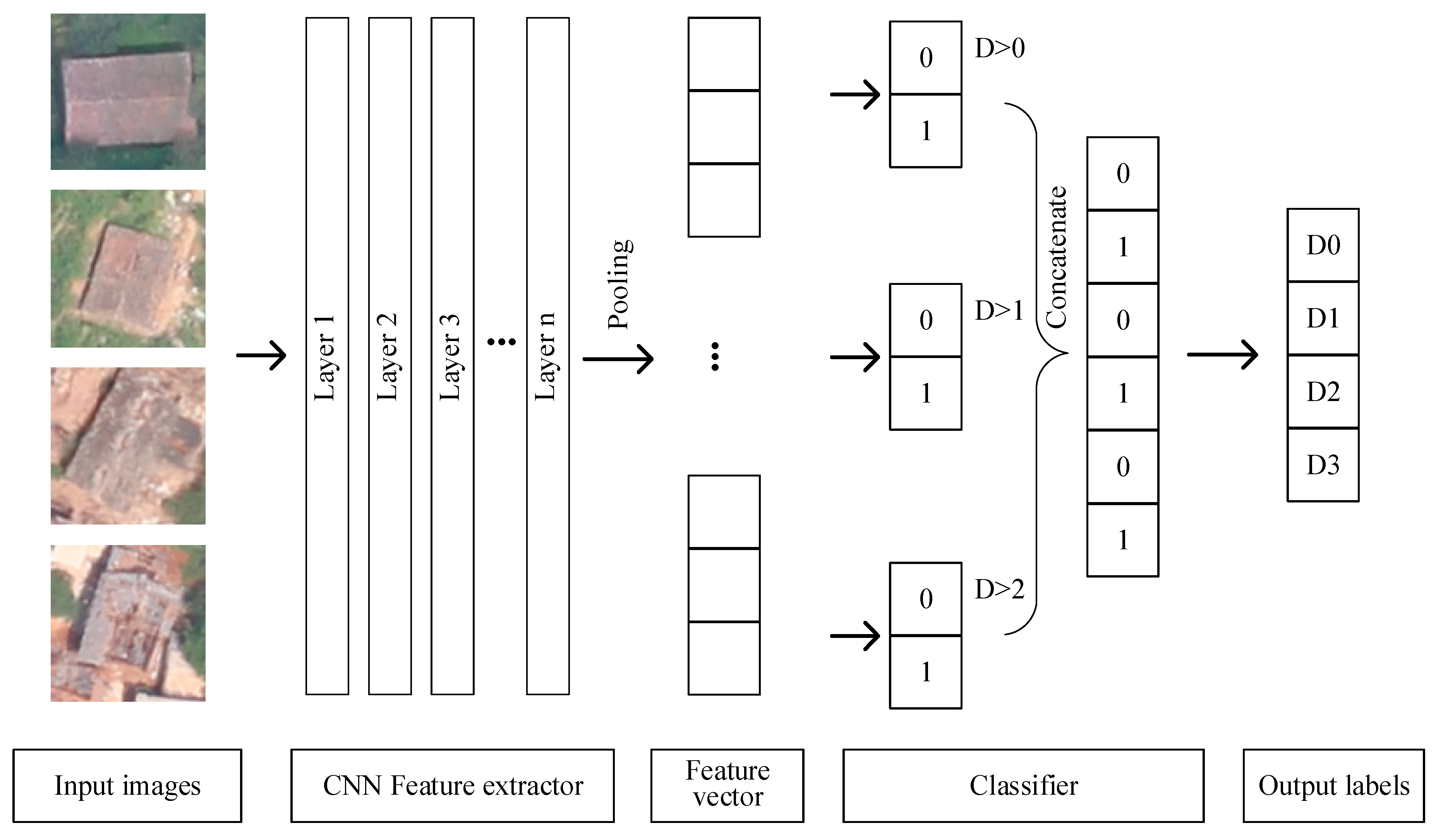
In this paper, we propose a new approach based on CNNs and ordinal regression (OR) aiming at assessing the degree of building damage caused by earthquakes with aerial imagery. CNNs hierarchically extract useful high-level features from input building images, and then OR is used to classify the features into four different damage grades. Then, we can get the degree of damaged buildings. The manually labeled damaged building dataset in this paper was obtained from aerial images after several historical earthquakes. The proposed mothed was evaluated with different network architecture and classifiers. We also compared the method with several state-of-the-art methods including hand-engineered features such as edge, texture, spectra, and morphology feature and machine learning methods.

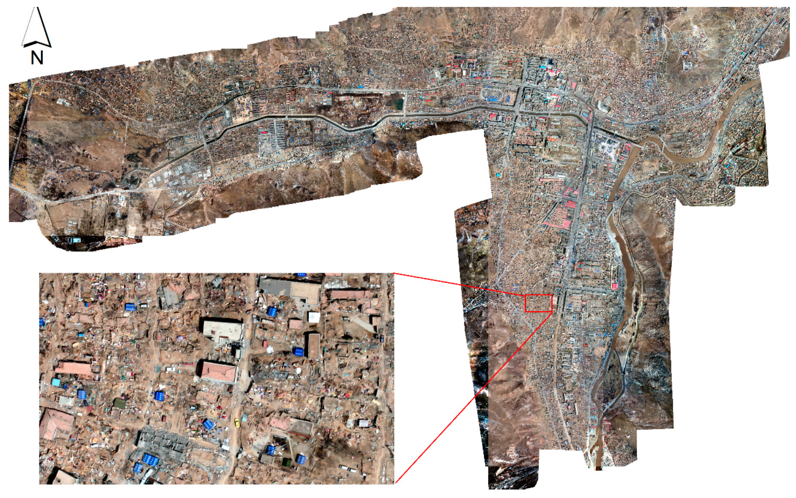
This is the first attempt to apply OR to assess the degree of building damage from aerial imagery. OR (also called ”ordinal classification”) is used to predict an ordinal variable. In this paper, the building damage degree, on a scale from “no observable damage” to “collapse”, is just an ordinal variable. However, typical multiclass classification ignores the ordered information between the damage degree, while damage degrees have a strong ordinal correlation. Thus, we cast the assessment problem of the degree building damage as an OR problem and develop an ordinal classifier and corresponding loss function to learn our network parameters. Information utilization was improved by OR, so we can achieve a better accuracy with the same or a lesser amount of data. When categorizing the damage to buildings into four types, we apply the method proposed in this paper to aerial images acquired from the 2014 Ludian earthquake and achieve an overall accuracy of 77.49%; when categorizing the damage to buildings into two types, the overall accuracy of the model is 93.95%, exceeding such values in similar types of theories and methods.

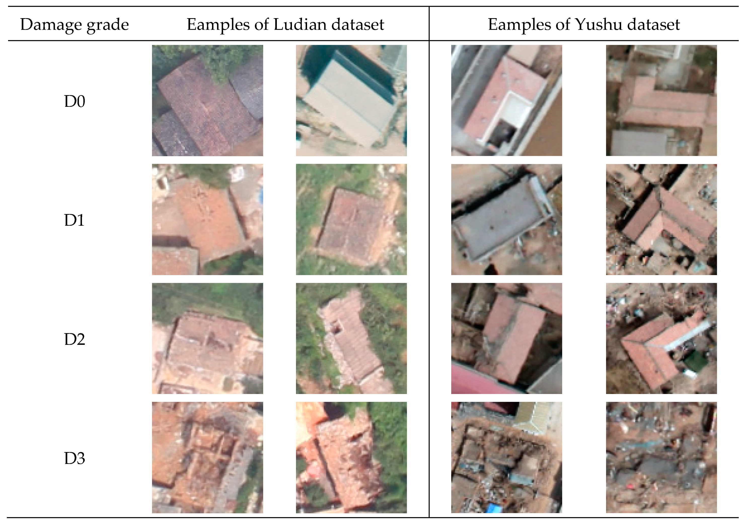
Another contribution of this work is a dataset of labeled building damage including 13,780 individual buildings from aerial data by visual interpretation that is classified into four damage degrees building by building.

The main contributions of this paper are summarized as follows:

(1) A deep ordinal regression network for assessing the degree of building damage caused by an earthquake. The proposed network uses a CNN for extracting features and an OR loss for optimizing classification results. Different CNNs’ architecture has also been evaluated.

(2) A dataset with more than 13,000 optical aerial images of labeled damage buildings can be download freely.

The rest of the paper is organized as follows: Section 2 presents an introduction to the dataset used in this research. Section 3 has a brief introduction to CNN and OR. Section 4 describes the proposed method and the different CNN architectures that we evaluated. We present the results of the experiments in Section 5. Finally, conclusions are drawn in Section 6.

2. Data

2.1. Remote Sensing Data

Two datasets from different seismic events were used in this study, including the Yushu earthquake in 2010 and Ludian earthquake in 2014, which are respectively described in the following text.

2.1.1. Images From Yushu Earthquake

On April 14 2010, Yushu County in Qinghai Province, China was hit by a 7.1-magnitude earthquake [25]. In this study, the aerial images with 0.1-m resolution on 16 April 2010 in Jiegu Town, the worst-hit area in the earthquake, was obtained. The data overview is shown in Figure 1, and the relevant parameters of the data are shown in

Table 1. Remote sensing imagery specifications.

Earthquake	Spatial Resolution (m)	Bands	Date
Ludian	0.2	R, G, B	7 and 14 August 2014
Yushu	0.1	R, G, B	16 April 16 2010

.

From the partial enlarged view corresponding to the red frame in Figure 1, a high building-collapse rate could be seen in the image-covered area, which was left in ruins. The details are clear, as the imaging quality is good.

2.1.2. Images From Ludian Earthquake

The 2014 Ludian earthquake was an Ms. 6.5 earthquake. The earthquake occurred on 3 August 2014 [26,27]. The earthquake caused major damage in Zhaotong City, Yunnan province. Aerial images were acquired to map the damage caused by the earthquake. Images acquired on 4 August 2014 were post-event airborne images for the remainder of the study. The aerial images have three spectral bands (R, G, and B) and a spatial resolution of 0.2 m. The images were georeferenced and mapped to a cartographic projection. On 7 and 14 August, after the earthquake, aerial remote sensing image data of the affected area was acquired. Figure 2 shows the range of the main aerial remote sensing image data acquired after the Ludian earthquake.

The data obtained in this paper mainly comes from the area with level $\mathrm{VIII}$ seismic intensity, Longtoushan Town and the northern bank of the Niulan River. The aerial remote sensing data of the Ludian earthquake (Figure 2) obtained in this paper was shot 4–10 days after the earthquake and has a spatial resolution of 0.2 m. With enough volume and good quality, it is suitable for damage degree assessment and the relevant study of single buildings.

Dominated by mountains, the Ludian region has a wide distribution of low-rise masonry–timber and soil–timber structures in villages. The spacing between buildings is large. The earthquake occurred in the summer; green trees can be seen and parts of the roofs of some houses are blocked by vegetation.

2.2. Dataset of Labeled Damage Building

In the research of DL image classification, a well-labeled dataset is very important, as it is used for training and evaluation benchmarks. Images of buildings at all levels of damage from the Ludian earthquake were used to construct the dataset. Each image was downsampled to 88 × 88. The size of the images is based on resolution and the length and width of local buildings.

The standard that we used to classify the damage degree is similar to EMS-98 [8], but with fewer levels. The damage degree D0 in this paper corresponds to G0-2 in EMS-98. D1 corresponds to G3 in EMS-98, and the rest can be done in the same manner. The standard can be found in

Table 2. Classification of damage to buildings in the Ludian earthquake.

Damage Grade	Description	Interpretation
D0	No observable damage	No cracking, breakage, etc.
D1	Light damage	Little cracking, breakage
D2	Heavy damage	Cracking in load-bearing elements with significant deformations across cracks
D3	Collapse	Collapse of complete structure or less of a floor

, and some samples of each damage level can found in Figure 3. We got about 13,780 individual buildings from remote sensing data of Ludian and 3501 buildings from Yushu by visual interpretation and classified them into four damage degrees building by building. When we labeled these samples, a few ground photos were used as a reference. These photos can help us better understand the actual damage to the buildings and the damage grade.

Before training the model, we needed to build a building dataset of different damage degrees. Thousands of building types were drawn by manual vectorization from the airborne images mentioned in Section 2.1.

Then, we intercepted each building into an image with a width and height of 88 pixels and placed the building in the center. Some samples can be found in Figure 3. In this paper, the damage terms “level”, “grade”, and “class” are used interchangeably. Building damage was classified into four classes.

Samples in the two datasets, Ludian and Yushu, have different characteristic. Datasets are named by their location where the data was obtained.

Table 3. Distribution of the samples in the two datasets.

Damage Grade	Number of Samples in the Ludian Dataset	Number of Samples in the Yushu Dataset
D0	2680	778
D1	5013	918
D2	2807	665
D3	3280	1140
Total	13,780	3501

shows the sample distribution of each damage grade.

2.3. Data Augmentation

In this paper, we have applied data augmentation [28] in order to artificially enlarge the dataset by using label-preserving transformations to the input data in order to generate new samples. Data augmentation can effectively avoid overfitting during the training of complex models and can significantly improve data quality. Several data augmentation techniques such as vertical and horizontal flipping, rotating at a certain degree (less than 15°), and increasing or reducing brightness were used. Examples can be found in

Table 4. Examples of data augmentation results.

Data Augmentation Examples
Original	Rotating clockwise by 90°	vertical flipping	horizontal flipping
Rotating 15° clockwise	Rotating 15° counterclockwise	Increasing the brightness	Reducing the brightness

.

3. Background Knowledge

3.1. Introduction to CNN

The convolution layer convolves the input image with a set of learnable filters, each producing one feature map in the output image. After crossing a nonlinear activation layer, it can get the picture feature of the next layer. The input feature map is compressed in the pooling layer. On the one hand, the pooling layer shrinks the feature map and simplifies the network-computing complexity. On the other hand, it compresses and extracts the main features. Generally, there are two kinds of operations in the pooling layer: max pooling and average pooling. In this paper, max pooling is adopted. The fully connected layer can connect all the features and convey results to the classifier.

Parameters of CNN can be obtained by training. The training includes two processes: forward and back propagation [29]. Forward propagation calculates the classification results of samples by current network weights. Back propagation compares the calculated classification results with true values, and then updates the network weights backward, layer by layer.

3.2. Ordinal Regression

In studies on machine learning and statistical models, classification is used to predict categories where targets belong based on input data. In classification, the relationship between categories is equal and independent, while the output is usually discrete. In typical classification, such as in the study of remote sensing land use and cover, the land surface is usually classified into vegetation, bare soil, water, buildings, and roads according to the spectrum, texture, and context of the surface features in the images [30,31]. In the recognition of handwritten figures [32], the given target images are classified into 0–9 classes. Although figures are used as class tags, there is no other relationship between any two classes. There are many commonly used methods to solve classification problems [33], including SVM [34], decision tree classifier [35], nearest neighbor algorithm [36], and CNN-based classification algorithms. The accuracy rate is the most commonly used index to describe the classification quality.

Regression analysis is used to predict the value of some property of the target based on input data and the output values are in a row within a value range. Guo et al. (2009) [37], based on images of faces, used a support vector regression (SVR) algorithm to predict the actual ages of people whose faces were shown. Human age is a continuous value with a limited value range, and is suitable for prediction by a regression algorithm. In studies related to image depth estimation, the distance (depth) between an object and a camera, as a continuous value, is usually estimated by a linear regression method in a machine learning algorithm, as shown in [38]. The commonly used methods to solve regression problems include the support vector regression algorithm and linear regression analysis. Variance, mean squared error, and other indices are often used to describe the regression quality.

Ordinal regression (OR) [39] is a statistical analysis model to predict ordinal tag variables corresponding to targets. OR is a statistical model between a classification and regression model. In other words, the original regression model prediction results are transformed into ordered discrete variables. For example, people’s ages are often expressed as positive integers, and they can also be predicted by an OR-based statistical learning model. For instance, Niu and Zhou et al. (2016) [40] used an OR model and CNNs to estimate age. In machine learning, OR can also be called ranked learning [41].

Table 5. Differences between regression, classification, and ordinal regression.

	Regression	Classification	Ordinal Regression
Type of output variables	Continuous data	Tag data or discrete data	Ordinal discrete data
Evaluation method	Mean squared error	Accuracy and confusion matrix	Mean squared error, accuracy, and confusion matrix
Example	People’s height	Categories of fruit	People’s age

lists the differences between regression, classification, and OR.

For OR problems, several original ordinal tag variables can be transformed into a set of binary classification subproblems [42]. By integrating the prediction results of all binary classification subproblems, the estimated results of an original OR problem can be obtained. Binary classifiers for ordinal regression can be solved by mature machine learning algorithms. In this study, the method to predict building damage degree is designed as a set of binary classification subproblems. For instance, OR was combined with CNNs for monocular depth estimation [43].

For ordinal tags including n classes and expressed by n natural numbers from 1 to n, when the tag corresponding to each target x is predicted, the original problem can be transformed to obtain n – 1 mapping relationships, each of which $f_i\left(x\right)$ means that the tag number y corresponding to the input x is less than or equal to probability i.

Using the characteristic extraction model of the image input to obtain the extracted advanced characteristic vector, the characteristic vector is imported into the classification model for classification.

4. Proposed Method

This section presents the details of the proposed “CNN in combination with OR” method. The proposed network is composed of two basic parts: a CNN feature extractor and classifier. These parts are discussed separately.

The CNN feature extractor includes several convolution layers followed by max-pooling and an activation function. The output of the CNN feature extractor is used as the feature vector of the classifier. The classifier usually consists of fully connected layers. An illustration of the proposed network is shown in Figure 4.

4.1. CNN Feature Extractor

CNN models are excellent in terms of representation learning. This feature makes them suitable for transfer learning, which consists of applying a model trained for a particular task to a different task. The transfer can be done by fine-tuning the existing weights of the network using the new dataset in order to adjust the model for a new target problem or by using the network as a feature extractor, which does not require retraining. In the latter case, an input sample is forwarded in order to obtain an intermediate representation, a vector; the vectors can be fed into other classifiers such as a Softmax classifier [44].

Two successful CNN models pretrained on ImageNet were evaluated as feature extractors in our work: the Visual Geometry Group Network (VGG) [45] and residual learning network (ResNet-50) [46]. Their parameters were initialized via the pretrained classification model on ImageNet Large Scale Visual Recognition Competition (ILSVRC) [47]. Fully connected layers in VGG-16 or ResNet-50 were removed and replaced with a new custom one that had 128 neurons. When the model was trained, all the convolutional layers were locked.

We design a baseline network to compare the performance. Every convolutional layer in this network is followed by Batch Normalization (BN) [48], Rectified Linear Unit (ReLU) [49] activation, and the max-pooling layer. The baseline is simple enough for us to preform initial configurations before using more complex topologies. A detailed description can be found in

Table 6. Description of baseline network. Conv-BN-ReLU is a block, consisting of a convolutional layer, BN layer, and RelU activation.

#	Layer	Kernel Size	Output Size
1	Conv-BN-ReLU	3	16 × 88 × 88
2	Maxpooling	2	16 × 44 × 44
3	Conv-BN-ReLU	3	32 × 44 × 44
4	Maxpooling	2	32 × 22 × 22
5	Conv-BN-ReLU	3	64 × 11 × 11
6	Maxpooling	2	64 × 11 × 11
7	Conv-BN-ReLU	3	128 × 11 × 11
8	Maxpooling	2	128 × 6 × 6
9	Conv-BN-ReLU	3	128 × 6 × 6
10	GlobalPooling		128

.

4.2. Classifier

As described in Section 2, in this study, buildings damaged by earthquakes can be classified into four damage degrees: D0, D1, D2, and D3. Based on this ordinal relationship, an OR-based building damage degree classifier model is proposed. For verification and comparison, the building assessment problem can be turned into a multiclass classification problem that adopts a Softmax classifier in a straightforward manner.

The Softmax classifier is a common softmax function that is used to divide the input data into four classes and give the probability of each class. The maximum probability is the prediction category of the current sample. The loss function of the Softmax classifier is the cross-entropy loss function.

The architecture of the OR classifier is shown in Figure 4. The OR classifier branches out three binary classification layers. Each binary classification layer corresponding to the probability of D > 0, D > 1, and D > 2. After that, we concatenate the three outputs into a single vector D$\left(d_0,d_1,\cdots ,d_5\right)$. The predicted damage degree is decoded from this vector.

It is assumed that $D=\phi \left(\chi ,\mathsf{\Theta }\right)$ means that the results vector D$\left(d_0,d_1,\cdots ,d_5\right)$ from the calculation with data input $\chi$ and model parameters $\mathsf{\Theta }$. Y$\left(y_0,y_1,\cdots ,y_5\right)$ means the actual vector that is encoded from the damage degree corresponding to data input $\chi$.

It is known from softmax function characteristics that

$$d_{2i}+d_{2i+1}=1$$

(1)

where $i\in \left\{0,1,2\right\}$.

Based on the definition, the following characteristics exist:

$$y_k\in \left\{0,1\right\}$$

(2)

$$y_{2i}+y_{2i+1}=1$$

(3)

where 0 ≤ k ≤ 5, $i\in \left\{0,1,2\right\}$.

The loss function $ℒ\left(Y,D\right)$ of the OR-based damage assessment model can be expressed as:

$$ℒ\left(Y,D\right)=-\frac{1}{3}{{\displaystyle \sum }}_{i=1}^3\left[y_{2i}log{d}_{2i}+\left(1-y_{2i}\right)log\left(1-d_{2i}\right)\right].$$

(4)

The loss function can be derived. Therefore, based on the back propagation algorithm, the minimum value of the loss function is obtained iteratively to result in the weight of the optimized model.

During prediction, for any sample input $\chi$, its dichotomous decomposition code D$\left(d_0,d_1,\cdots ,d_5\right)$ can be decoded to the corresponding damage degree $\hat{d}$ by the following method:

$$\widehat{d}={\displaystyle {\displaystyle \sum }_{i=0}^3}\psi \left(d_{2i}\ge 0.5\right)$$

(5)

where the indicator function $\psi$ can be expressed as

$$\{\begin{array}{c}\psi \left(true\right) = 1\\ \psi \left(false\right) = 0\end{array}.$$

(6)

4.3. Evaluated Networks

In this work, we evaluated six CNN topologies with different feature extractors and classifiers. The name and composition of each network can be found in

Table 7. Network topologies to be evaluated. Each network consists of a feature extractor and a classifier. ResNet: residual learning network.

Name	Feature Extractor	Classifier	Para Num.
Baseline-SC	Baseline	Softmax classifier	57,254
Baseline-OR	Baseline	OR classifier	57,510
VGG-SC	VGG	Softmax classifier	7,833,670
VGG-OR	VGG	OR classifier	7,833,926
ResNet-SC	ResNet-50	Softmax classifier	23,851,014
ResNet-OR	ResNet-50	OR classifier	23,851,270

. The two classification methods are the Softmax classifier (SC) and the ordinal regression classifier. All of these network topologies will be evaluated.

4.4. Model Realization

In this section, the DL model algorithm was programmed by Keras [50] and a TensorFlow [51] open-source DL framework and the Python 3.6 programming language [52]. All experimental and test codes were run on the same computer platform. The hardware configuration of the computer consisted of an Intel i7 3.4 GHz CPU, 16.0 GB memory, GeForce RTX 2080 Ti graphics, and 8 G RAM display. The operating system was Ubuntu 18.04. CUDA version 9.0 [53] was used for acceleration computing. The GDAL2.2.2 geographic data processing software package [54] was used to read and write image data, conduct vector operations, and transform geographic projections.

The pretrained weight based on the ImageNet dataset is widely used in transfer learning because characteristics such as the edge, texture, and structure learned from the ImageNet dataset are universal in computer vision tasks [55]. The weight initialization of the VGG and ResNet characteristic extraction modules employs the pretrained weight based on the ImageNet dataset. In the baseline feature extractor, the weight initialization is conducted by Glorot uniform distribution initialization [56]. All models use the same training dataset for training.

The stochastic gradient descent (SGD) method [57] is a common optimization algorithm in DL model training [58]. In this paper, the SGD algorithm with momentum [59] is used for model training.

4.5. Model Evaluation Methods and Indicators

4.5.1. Confusion Matrix

A confusion matrix is used to judge the consistency between the classification results of models or classifiers and the true category information, and is one of the basic evaluation methods for remote sensing image classification. The specific procedure is to compare the classification result tags with the true category information one by one, and C is used to represent the confusion matrix. It is assumed that there are K classes of samples, and that C is a row K and column K matrix. Any C (i, j) represents the true category i and the total samples in the predicted category j.

4.5.2. Overall Accuracy and Kappa Coefficient

Overall accuracy (OA) refers to the consistency probability between classification results and true classes. Its calculation formula is

$$OA=\frac{{{\displaystyle \sum }}_i^{K}C\left(i,i\right)}{{{\displaystyle \sum }}_i^K{{\displaystyle \sum }}_j^{K}C\left(i,j\right)}.$$

(7)

The kappa coefficient [60] is calculated based on the confusion matrix to measure the calculation indicator of classification accuracy. The theoretical kappa coefficient falls between [–1, 1], but the actual value is often between [0, 1]. Its calculation formula is

$$p_e=\frac{{{\displaystyle \sum }}_i^K\left({{\displaystyle \sum }}_j^{K}C\left(i,j\right)\ast {{\displaystyle \sum }}_j^{K}C\left(j,i\right)\right)}{N^2}$$

(8)

$$Kappa=\frac{OA-p_e}{1-p_e}$$

(9)

where N is the total number of samples.

4.5.3. Mean Squared Error

In statistics, the mean squared error (MSE) or mean squared deviation (MSD) of an estimator measures the average of the squares of the errors—that is, the average squared difference between the estimated values and the actual value. The mean squared error is the average of the quadratic sum of the error between the predicted data and true values. Its calculation formula is

$$MSE=\frac{1}{N}{\displaystyle {\displaystyle \sum }_{i=1}^N}{\left(y_i-{\widehat{y}}_i\right)}^2$$

(10)

where $y_i$ is the true value, ${\hat{y}}_i$ is the predicted value, and N is the total number of samples.

In this study, MSE may be a more important indicator than overall accuracy. For example,

Table 8. Two confusion matrixes with the same overall accuracy (OA) and different mean squared errors (MSEs).

Confusion Matrixes 1					Confusion Matrixes 2
	A	B	C	D		A	B	C	D
A	10	8	6	4	A	10	6	8	6
B	8	10	8	6	B	6	10	6	8
C	6	8	10	8	C	8	6	10	6
D	4	6	8	10	D	6	8	6	10
OA	0.3333				OA	0.3333
Kappa	0.1098				Kappa	0.1111
MSE	1.8				MSE	2.2667

shows two confusion matrixes, which have same overall accuracy and different mean squared errors. In this study, Confusion matrix 1 is better than Confusion matrix 2, but OA does not reflect this situation. We need MSE to evaluate our model.

5. Results

5.1. Dataset Configuration

During the model training, each dataset prepared in Section 2 was divided into three parts at a proportion of 8:1:1. Then, 80% of the sample data was randomly selected for the training set, 10% was randomly selected for the Validation set, and 10% was randomly selected for the testing set. The amount of building damage classification is guaranteed to be balanced in each set. Fivefold cross-validation was applied to evaluate the model.

The two datasets mentioned in this paper, the Ludian dataset and Yushu dataset, have different uses. Among them, the Ludian dataset with more data is used to train the model, while the Yushu dataset with less data is used to verify the adaptability of the model.

During the training, the data of the training sets included four damage degrees, as shown in Section 2: complete damage, severe damage, common, and nearly intact. The validation set and testing set also included the four classes above. The training set was used to input models to make them automatically adjust the weight parameters based on the back propagation algorithm. The verification set was used for model seletion. The testing set was used to verify the actual model accuracy. The following accuracy and kappa coefficient calculation results were obtained from the data of the testing set.

As the buildings to be evaluated are classified as damaged or not damaged in most current studies, in this paper, three sets were created by grouping samples of different damage degrees (

Table 9. Distribution of three damage grade sets.

Set	Subclass	Damage Grade
1	Nearly intact	D0, D1, D2
	damaged	D3
2	Nearly intact	D0, D1
	Severe damage	D2
	Complete collapse	D3
3	No observable damage	D0
	Light damage	D1
	Heavy damaged	D2
	Collapse	D3

). In Set 1, D0, D1, and D2 were incorporated into an intact class and D3 was incorporated into a damaged class to compare with other methods; in Set 2, D0 and D1 were incorporated into a nearly intact class, D2 was incorporated into a severe damage class, and D3 was incorporated into a complete collapse class. The prediction results of models will be recalculated again to compare the evaluation indicators.

5.2. Accuracy Results on Ludian Dataset

As shown in

Table 10. Accuracy indicators of deep learning (DL) models. The last rows show the average values. The best result for each classifier and set is shown in bold type.

Model	Set 1			Set 2			Set 3
	OA	Kappa	MSE	OA	Kappa	MSE	OA	Kappa	MSE
Baseline-SC	92.40%	0.78	0.08	82.73%	0.71	0.20	72.86%	0.62	0.30
VGG-SC	93.66%	0.82	0.06	85.05%	0.74	0.20	75.10%	0.66	0.28
ResNet-SC	92.99%	0.80	0.08	83.16%	0.71	0.22	74.31%	0.64	0.31
Average	93.02%	0.80	0.07	83.65%	0.72	0.21	74.09%	0.64	0.30
Baseline-OR	92.40%	0.79	0.08	82.81%	0.71	0.21	73.73%	0.64	0.32
VGG-OR	93.95%	0.83	0.06	85.46%	0.75	0.17	77.39%	0.69	0.25
ResNet-OR	93.81%	0.82	0.07	84.71%	0.72	0.19	75.05%	0.66	0.30
Average	93.39%	0.81	0.07	84.33%	0.73	0.19	75.39%	0.66	0.29

, for Set 3, the minimum overall accuracy of the six network models is 72.86% for Baseline-SC, and the average is 74.09%. The accuracy is 77.39% for VGG-OR, in which the maximum value, with a kappa coefficient of 0.69, represents good model consistency. For Set 1, the accuracy of all the models is about 92%–94% and the average is 93%, with a small fluctuation. The best accuracy is 93.95% for VGG-OR. The kappa coefficient, ranging between 0.78 and 0.83, representing very good model consistency.

In statistical modeling, the MSE can represent the difference between the actual observations and the observation values predicted by the model. So, when the overall accuracy is equal to or lower than the MSE, the better the model performance. It makes a lot of sense to minimize the MSE in the damage degree assessment to buildings. Table 10 shows that the MSE results of the OR approach are always better than the values of direct classification methods, which can be explained because more ordinal information can avoid bias.

According to the results of the comparison shown in Table 10, it is possible to affirm that our OR approach (VGG-OR) outperforms the direct classification methods.

We set the learning rate as 0.001, and the batch size was set to 32. Models with same CNN feature extractor take the same amount of time, because the OR classifier does not consume more computing resources. The baseline, VGG, and ResNet models require 6, 10, and 33 min, respectively, for 100 epochs of iterations using the same training dataset. Models usually converge within 100 epochs. It can be concluded that VGG-OR gains 3.66% increments over Baseline-OR with the cost of only a 4-minute increment of model training time.

In order to check whether the results are stable, the standard deviation (SD) of OA, Kappa, and MSE is shown in

Table 11. The standard deviation (SD) of OA, Kappa, and MSE of deep learning (DL) models on Set 3.

Model	Set 3
	SD for OA	SD for Kappa	SD for MSE
Baseline-SC	0.0122	0.0188	0.0154
VGG-SC	0.0064	0.0099	0.0081
ResNet-SC	0.0152	0.0234	0.0191
Baseline-OR	0.0086	0.0133	0.0108
VGG-OR	0.0056	0.0086	0.0070
ResNet-OR	0.0112	0.0173	0.0141

. Since the metrics of Set 1 and Set 2 are calculated from Set 3, only the SD of the metrics of Set 3 is shown in Table 11. All the SD values are quite small, which means that the results of models can be obtained relatively stably.

5.3. Accuracy Results on Yudian Dataset

Given that the amount of data in the Yushu dataset is much smaller than that of the Ludian dataset, it is less effective in training the model. Therefore, we attempted to transfer the model trained by the Ludian dataset to the Yushu dataset. Firstly, the effects of the model trained with the Ludian dataset applied directly to the Yushu dataset were verified, as shown in

Table 12. Accuracy indicators of the model trained with the Ludian dataset applied directly to the Yushu dataset.

Set	OA	Kappa	MSE
Set 1	90.14%	0.80	0.10
Set 2	74.43%	0.60	0.32
Set 3	64.28%	0.49	0.52

.

It can be found that all the indicators demonstrate a significant decline, and the accuracy is only 64%, suggesting an invalid model. This indicates that there is a difference in the data distribution rules between the two datasets, so the model trained by one dataset is not applicable to the other.

Then, we tried to transfer the model trained by the Ludian dataset to the Yushu dataset. Through parameter fine-tuning, a learning rate of 0.0001 was adopted, and all the layers except for the full connection layer were locked. As a contrast, the model was also directly trained by the Yushu dataset. The actual number of training set samples was controlled to analyze the impact of the input data on the model performance.

Figure 5 shows the impact of the number of training set samples on the overall accuracy, and the error bar represents the SD value. The model that was transfered from the Ludian dataset is more accurate and more stable.

6. Discussion

The proposed method is an "end-to-end" solution. The input to this method is the sample image data, and the output is the damage level label. The method can directly obtain the available results without worrying about intermediate products. Considering the damage level of a building as an OR problem with ordered labels, it can make more effective use of model input information, which can improve the accuracy of the model and reduce the MSE of the prediction results. The deep learning-based algorithm model applied in this paper can also be regarded as a data-driven method. This means that the larger the dataset, the better the model performance.

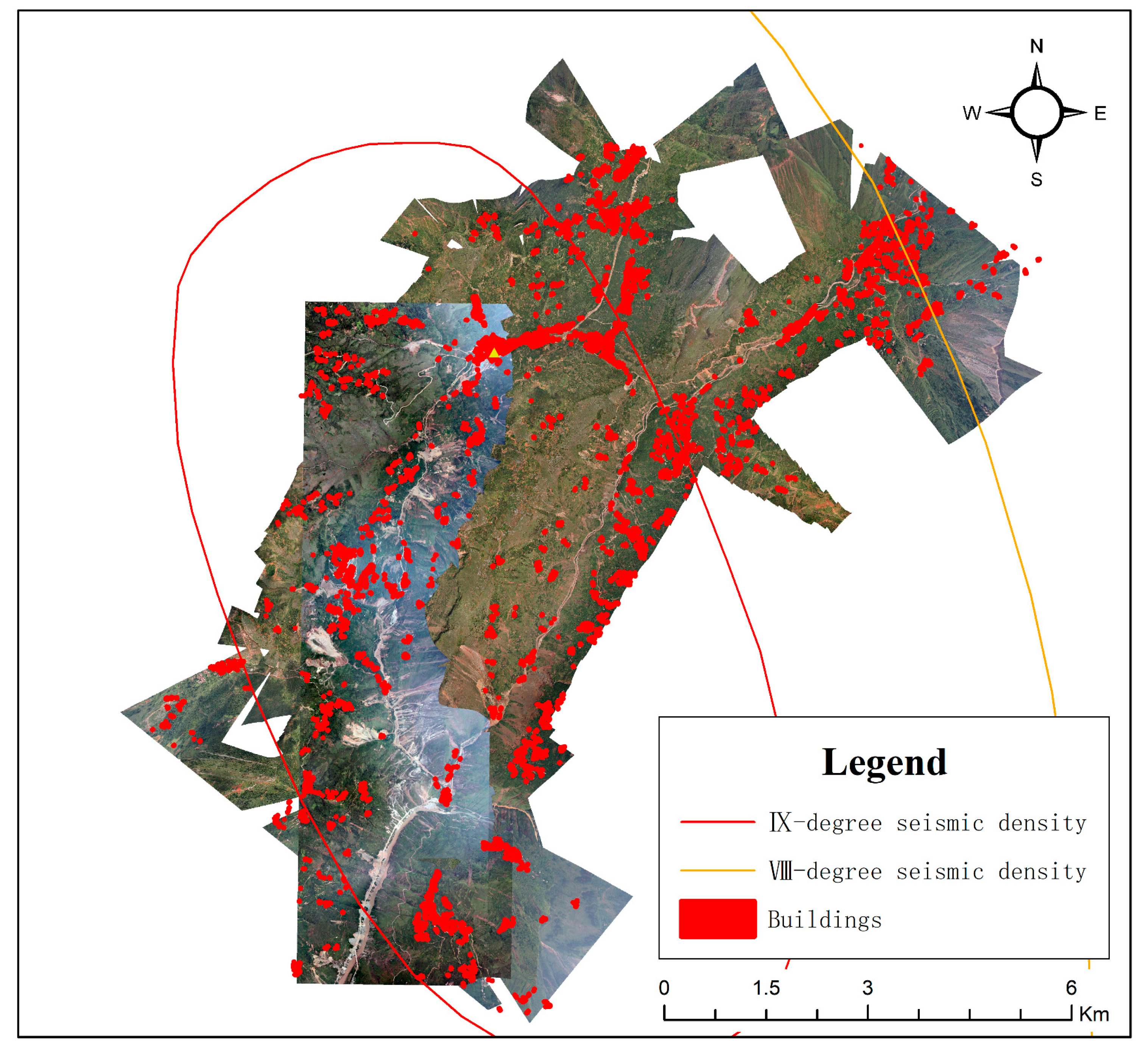
In this study, we try to transfer the model between datasets of labeled damage buildings acquired from different earthquake locations. The datasets share the same damage levels but have different data characteristics. They are similar but not the same, so a model trained with one cannot be used for the other. The transfer learning experiment not only verified a method to solve the problem of a lack of data, but also proved the stability of the model in different regions.

In the study of machine learning, it is commonly accepted that the more samples for the training model there are, the better, but it does not mean that increasing the data of one model will definitely lead to an obvious performance improvement. When there are few samples, the performance of the algorithm based on DL may not be good because the algorithm needs a large amount of parameters in many data-training models. Correspondingly, if there is less data, the performance of the machine learning algorithm based on manual characteristic selection may be better with customized rules and the help of professionals. With a huge amount of data, the performance of the DL algorithm will increase with the increasing data scale.

CNN models are developed by training the network to represent the relationships and processes that are inherent within the datasets. They perform an input–output mapping using a set of interconnected simple processing features. We should realize that such models typically do not really represent the physics of a modeled process; they are just devices used to capture relationships between the relevant input and output variables [61]. These models can also be considered as data-driven models. So, the amount and quality of an input dataset may influence the upper limit of the model performance.

A critical factor for the use of proposed model is data availability. The amount of well-labeled samples should be enough. In the case study of the Yushu dataset, 1500 or more images are needed in the training set, and the validation and testing sets also need some data. This number can go down significantly if a pretrained model is used.

In this study, four damage grades were adopted. However, the visual interpretation of aerial images includes uncertainty or mis-classification especially for light and heavy damage levels [6]. The damage degree will be underestimated by aerial images (Figure 6). A Bayesian updating process is discussed in [6] to reduce uncertainties with ground truth data.

7. Conclusions

The study was carried out on the high-precision and automated assessment method of damage to buildings; the entire process, including experimental data preparation, dataset construction, detailed model implementation, verification by experiment, and assessment and verification, was systematically conducted; and the performance of the model in practical applications was predicted through independent and disparate datasets, applying and validating the strengths and potential of the proposed assessment method.

We propose a new approach based on CNNs and OR aiming at assessing the degree of building damage caused by earthquakes with aerial imagery. The network consists of a CNN feature extractor and an OR classifier. This is the first attempt to apply OR to assess the degree of building damage from aerial imagery. Information utilization was improved by OR, so we can achieve a better accuracy with the same or a lesser amount of data. As the buildings to be evaluated are classified as damaged or not damaged in most current studies, we recalculate the evaluation indicators in the case of two classes and three classes. The proposed method significantly outperforms previous approaches.

In this study, we produced a new dataset that consisted of labeled images of damaged buildings. More than 13,000 optical aerial images were classified into four damage degrees based on the damage scale in Table 3. The dataset and code are freely available online and can be found at [62].

In the future, we will attempt to expand the training data on more sensors and types of buildings. A transfer learning algorithm will also be considered when lacking training data. Based on the existing classification model, combined with the object detection algorithm, such as RetinaNet [63], the end-to-end automatic extraction of damaged building locations and corresponding damage levels within the image range can be achieved, further reducing the intermediate process. We would apply our method to more extensive and diverse types of remote sensing data. OR method has great potential to be widely used in other ordinal-scale signals, such as sea ice concentration.

References

1. Dong, L.; Shan, J. A comprehensive review of earthquake-induced building damage detection with remote sensing techniques. ISPRS J. Photogramm. Remote Sens. 2013, 84, 85–99. [Google Scholar] [CrossRef]
2. Tian, T.; Nielsen, A.A.; Reinartz, P. Building Damage Assessment after the Earthquake in Haiti using two Post-Event Satellite Stereo imagery and DSMs. Int. J. Image Data Fusion 2015, 6, 155–169. [Google Scholar] [CrossRef]
3. Klonus, S.; Tomowski, D.; Ehlers, M.; Reinartz, P.; Michel, U. Combined Edge Segment Texture Analysis for the Detection of Damaged Buildings in Crisis Areas. IEEE J. Sel. Top. Appl. Earth Obs. Remote Sens. 2012, 5, 1118–1128. [Google Scholar] [CrossRef]
4. Chen, Z.; Hutchinson, T.C. Structural damage detection using bi-temporal optical satellite images. Int. J. Remote Sens. 2011, 32, 4973–4997. [Google Scholar] [CrossRef]
5. Vu, T.T.; Ban, Y. Context-based mapping of damaged buildings from high-resolution optical satellite images. Int. J. Remote Sens. 2010, 31, 3411–3425. [Google Scholar] [CrossRef]
6. Booth, E.; Saito, K.; Spence, R.; Madabhushi, G.; Eguchi, R.T. Validating assessments of seismic damage made from remote sensing. Earthq. Spectra 2011, 27, S157–S177. [Google Scholar] [CrossRef]
7. Saito, K.; Spence, R.; de C Foley, T. Visual damage assessment using high-resolution satellite images following the 2003 Bam, Iran, earthquake. Earthq. Spectra 2005, 21, 309–318. [Google Scholar] [CrossRef]
8. Grünthal, G. European Macroseismic Scale 1998; European Seismological Commission (ESC): Luxembourg City, Luxembourg, 1998. [Google Scholar]
9. Huyck, C.K.; Adams, B.J.; Cho, S.; Chung, H.-C.; Eguchi, R.T. Towards rapid citywide damage mapping using neighborhood edge dissimilarities in very high-resolution optical satellite imagery—Application to the 2003 Bam, Iran, earthquake. Earthq. Spectra 2005, 21, 255–266. [Google Scholar] [CrossRef]
10. Adams, B. Improved disaster management through post-earthquake building damage assessment using multitemporal satellite imagery. In Proceedings of the ISPRS XXth Congress, Istanbul, Turkey, 12–23 July 2004; Volume 35, pp. 12–23. [Google Scholar]
11. Anniballe, R.; Noto, F.; Scalia, T.; Bignami, C.; Stramondo, S.; Chini, M.; Pierdicca, N. Earthquake damage mapping: An overall assessment of ground surveys and VHR image change detection after L’Aquila 2009 earthquake. Remote Sens. Environ. 2018, 210, 166–178. [Google Scholar] [CrossRef]
12. Plank, S. Rapid Damage Assessment by Means of Multi-Temporal SAR—A Comprehensive Review and Outlook to Sentinel-1. Remote Sens. 2014, 6, 4870–4906. [Google Scholar] [CrossRef]
13. Gupta, R.; Goodman, B.; Patel, N.; Hosfelt, R.; Sajeev, S.; Heim, E.; Doshi, J.; Lucas, K.; Choset, H.; Gaston, M. Creating xBD: A Dataset for Assessing Building Damage from Satellite Imagery. In Proceedings of the IEEE Conference on Computer Vision and Pattern Recognition Workshops, Long Beach, CA, USA, 16–20 June 2019; pp. 10–17. [Google Scholar]
14. Li, P.; Xu, H.; Guo, J. Urban building damage detection from very high resolution imagery using OCSVM and spatial features. Int. J. Remote Sens. 2010, 31, 3393–3409. [Google Scholar] [CrossRef]
15. Yu, H.; Cheng, G.; Ge, X. Earthquake-collapsed building extraction from LiDAR and aerophotograph based on OBIA. In Proceedings of the 2nd International Conference on Information Science and Engineering, Hangzhou, China, 4–6 December 2010; pp. 2034–2037. [Google Scholar]
16. Cooner, A.; Shao, Y.; Campbell, J. Detection of Urban Damage Using Remote Sensing and Machine Learning Algorithms: Revisiting the 2010 Haiti Earthquake. Remote Sens. 2016, 8, 868. [Google Scholar] [CrossRef]
17. Ji, M.; Liu, L.; Buchroithner, M. Identifying Collapsed Buildings Using Post-Earthquake Satellite Imagery and Convolutional Neural Networks: A Case Study of the 2010 Haiti Earthquake. Remote Sens. 2018, 10, 1689. [Google Scholar] [CrossRef]
18. Duarte, D.; Nex, F.; Kerle, N.; Vosselman, G. Multi-Resolution Feature Fusion for Image Classification of Building Damages with Convolutional Neural Networks. Remote Sens. 2018, 10, 1636. [Google Scholar] [CrossRef]
19. Maggiori, E.; Tarabalka, Y.; Charpiat, G.; Alliez, P. Convolutional Neural Networks for Large-Scale Remote Sensing Image Classification. IEEE Trans. Geosci. Remote Sens. 2016, 55, 645–657. [Google Scholar] [CrossRef]
20. Scott, G.J.; England, M.R.; Starms, W.A.; Marcum, R.A.; Davis, C.H. Training Deep Convolutional Neural Networks for Land 2013; Cover Classification of High-Resolution Imagery. IEEE Geosci. Remote Sens. Lett. 2017, 14, 549–553. [Google Scholar] [CrossRef]
21. Zou, Q.; Ni, L.; Zhang, T.; Wang, Q. Deep Learning Based Feature Selection for Remote Sensing Scene Classification. IEEE Geosci. Remote Sens. Lett. 2015, 12, 2321–2325. [Google Scholar] [CrossRef]
22. Zhang, X.; Chen, G.; Wang, W.; Wang, Q.; Dai, F. Object-Based Land-Cover Supervised Classification for Very-High-Resolution UAV Images Using Stacked Denoising Autoencoders. IEEE J. Sel. Top. Appl. Earth Obs. Remote Sens. 2017, 10, 3373–3385. [Google Scholar] [CrossRef]
23. Xie, F.; Shi, M.; Shi, Z.; Yin, J.; Zhao, D. Multilevel Cloud Detection in Remote Sensing Images Based on Deep Learning. IEEE J. Sel. Top. Appl. Earth Obs. Remote Sens. 2017, 10, 3631–3640. [Google Scholar] [CrossRef]
24. Gallego, A.-J.; Pertusa, A.; Gil, P. Automatic Ship Classification from Optical Aerial Images with Convolutional Neural Networks. Remote Sens. 2018, 10, 511. [Google Scholar] [CrossRef]
25. Guo, H.; Zhang, B.; Lei, L.; Zhang, L.; Chen, Y. Spatial distribution and inducement of collapsed buildings in Yushu earthquake based on remote sensing analysis. Sci. China Earth Sci. 2010, 53, 794–796. [Google Scholar] [CrossRef]
26. Fan, Y.; Wen, Q.; Wang, W.; Wang, P.; Li, L.; Zhang, P. Quantifying Disaster Physical Damage Using Remote Sensing Data—A Technical Work Flow and Case Study of the 2014 Ludian Earthquake in China. Int. J. Disaster Risk Sci. 2017, 8, 471–488. [Google Scholar] [CrossRef]
27. Xu, P.; Wen, R.; Wang, H.; Ji, K.; Ren, Y. Characteristics of strong motions and damage implications of M S6.5 Ludian earthquake on August 3, 2014. Earthq. Sci. 2015, 28, 17–24. [Google Scholar] [CrossRef]
28. Krizhevsky, A.; Sutskever, I.; Hinton, G.E. ImageNet Classification with Deep Convolutional Neural Networks. In Advances in Neural Information Processing Systems; Lake Tahoe, USA; MIT Press: Cambridge, MA, USA, 2012. [Google Scholar]
29. Rumelhart, D.E.; Hinton, G.E.; Williams, R.J. Learning representations by back-propagating errors. Nature 1986, 323, 533. [Google Scholar] [CrossRef]
30. Castelluccio, M.; Poggi, G.; Sansone, C.; Verdoliva, L. Training convolutional neural networks for semantic classification of remote sensing imagery. In Proceedings of the 2017 Joint Urban Remote Sensing Event (JURSE), Dubai, UAE, 6–8 March 2017; pp. 1–4. [Google Scholar]
31. Wang, Y.; Gu, L.; Ren, R.; Zheng, X.; Fan, X. A land-cover classification method of high-resolution remote sensing imagery based on convolution neural network. In Proceedings of the Earth Observing Systems XXIII, San Diego, CA, USA, 7 September 2018; p. 107641Y. [Google Scholar]
32. LeCun, Y.; Cortes, C.; Burges, C. MNIST Handwritten Digit Database. Available online: http://yann.lecun.com/exdb/mnist (accessed on 28 November 2019).
33. Wu, X.; Kumar, V.; Quinlan, J.R.; Ghosh, J.; Yang, Q.; Motoda, H.; McLachlan, G.J.; Ng, A.; Liu, B.; Philip, S.Y.; et al. Top 10 algorithms in data mining. Knowl. Inf. Syst. 2008, 14, 1–37. [Google Scholar] [CrossRef]
34. Mountrakis, G.; Im, J.; Ogole, C. Support vector machines in remote sensing: A review. ISPRS J. Photogramm. Remote Sens. 2011, 66, 247–259. [Google Scholar] [CrossRef]
35. Safavian, S.R.; Landgrebe, D. A survey of decision tree classifier methodology. IEEE Trans. Syst. Man Cybern. 1991, 21, 660–674. [Google Scholar] [CrossRef]
36. Thanh Noi, P.; Kappas, M. Comparison of random forest, k-nearest neighbor, and support vector machine classifiers for land cover classification using Sentinel-2 imagery. Sensors 2018, 18, 18. [Google Scholar] [CrossRef]
37. Guo, G.; Fu, Y.; Dyer, C.R.; Huang, T.S. Image-based human age estimation by manifold learning and locally adjusted robust regression. IEEE Trans. Image Process. 2008, 17, 1178–1188. [Google Scholar]
38. Eigen, D.; Puhrsch, C.; Fergus, R. Depth map prediction from a single image using a multi-scale deep network. In Proceedings of the Advances in Neural Information Processing Systems, Montreal, Canada, 8–13 December 2014; pp. 2366–2374. [Google Scholar]
39. Greco, S.; Mousseau, V.; Słowiński, R. Ordinal regression revisited: Multiple criteria ranking using a set of additive value functions. Eur. J. Oper. Res. 2008, 191, 416–436. [Google Scholar] [CrossRef]
40. Niu, Z.; Zhou, M.; Wang, L.; Gao, X.; Hua, G. Ordinal regression with multiple output cnn for age estimation. In Proceedings of the IEEE Conference on Computer Vision and Pattern Recognition, Les Vegas, NV, USA, 26 June–1 July 2016; pp. 4920–4928. [Google Scholar]
41. Shashua, A.; Levin, A. Ranking with large margin principle: Two approaches. In Advances in Neural Information Processing Systems; MIT Press: Cambridge, MA, USA, 2003. [Google Scholar]
42. Li, L.; Lin, H.-T. Ordinal regression by extended binary classification. In Proceedings of the Advances in Neural Information Processing Systems, Columbia, Canada, 4–7 December 2006; pp. 865–872. [Google Scholar]
43. Fu, H.; Gong, M.; Wang, C.; Batmanghelich, K.; Tao, D. Deep Ordinal Regression Network for Monocular Depth Estimation. In Proceedings of the IEEE Conference on Computer Vision and Pattern Recognition, Salt Lake, UT, USA, 18–22 June 2018; pp. 2002–2011. [Google Scholar]
44. Nasrabadi, N.M. Pattern recognition and machine learning. J. Electron. Imaging 2007, 16, 049901. [Google Scholar]
45. Simonyan, K.; Zisserman, A. Very Deep Convolutional Networks for Large-Scale Image Recognition. arXiv 2015, arXiv:1409.1556v6. [Google Scholar]
46. He, K.; Zhang, X.; Ren, S.; Sun, J. Deep Residual Learning for Image Recognition. In Proceedings of the Computer Vision and Pattern Recognition, Les Vegas, NV, USA, 26 June–1 July 2016; pp. 770–778. [Google Scholar]
47. Russakovsky, O.; Deng, J.; Su, H.; Krause, J.; Satheesh, S.; Ma, S.; Huang, Z.; Karpathy, A.; Khosla, A.; Bernstein, M.; et al. Imagenet large scale visual recognition challenge. Int. J. Comput. Vis. 2015, 115, 211–252. [Google Scholar] [CrossRef]
48. Ioffe, S.; Szegedy, C. Batch Normalization: Accelerating Deep Network Training by Reducing Internal Covariate Shift. arXiv 2015, arXiv:1502.03167. [Google Scholar]
49. Nair, V.; Hinton, G.E. Rectified linear units improve restricted boltzmann machines. In Proceedings of the 27th International Conference on Machine Learning (ICML-10), Haifa, Israel, 21–24 June 2010; pp. 807–814. [Google Scholar]
50. Chollet, F. Keras. In GitHub; 2015. Available online: https://github.com/fchollet/keras (accessed on 28 November 2019).
51. Abadi, M.; Agarwal, A.; Barham, P.; Brevdo, E.; Chen, Z.; Citro, C.; Corrado, G.S.; Davis, A.; Dean, J.; Devin, M.; et al. TensorFlow: Large-Scale Machine Learning on Heterogeneous Systems; In GitHub; 2015. Available online: https: //www.tensorflow.org/ (accessed on 28 November 2019).
52. Sanner, M.F. Python: A programming language for software integration and development. J. Mol. Graph. Model. 1999, 17, 57–61. [Google Scholar]
53. Nvidia, C. Compute Unified Device Architecture Programming Guide; NVIDIA Corporation. Available online: http://docs.nvidia.com/cuda (accessed on 28 November 2019).
54. Warmerdam, F. The geospatial data abstraction library. In Open Source Approaches in Spatial Data Handling; Springer: Berlin, Heidelberg, 2008; Volume 2, pp. 87–104. [Google Scholar]
55. Huh, M.; Agrawal, P.; Efros, A.A. What Makes ImageNet Good for Transfer Learning? Available online: https://arxiv.org/abs/1608.08614 (accessed on 28 November 2019).
56. Glorot, X.; Bengio, Y. Understanding the difficulty of training deep feedforward neural networks. In Proceedings of the Thirteenth International Conference on Artificial Intelligence and statistics, Sardinia, Italy, 13–15 May 2010; pp. 249–256. [Google Scholar]
57. Bottou, L. Large-scale machine learning with stochastic gradient descent. In Proceedings of the COMPSTAT’2010; Lechevallier, Y., Saporta, G., Eds.; Springer: Berlin, Germany, 2010; pp. 177–186. [Google Scholar]
58. Ruder, S. An overview of gradient descent optimization algorithms. arXiv 2016, arXiv:1609.04747. [Google Scholar]
59. Sutskever, I.; Martens, J.; Dahl, G.; Hinton, G. On the importance of initialization and momentum in deep learning. In Proceedings of the International conference on machine learning, Atlanta, GA, USA, 16 July 2018; pp. 1139–1147. [Google Scholar]
60. Cohen, J. A Coefficient of Agreement for Nominal Scales. Educ. Psychol. Meas. 1960, 20, 37–46. [Google Scholar] [CrossRef]
61. Solomatine, D.P.; See, L.M.; Abrahart, R.J. Chapter 2 Data-Driven Modelling: Concepts, Approaches and Experiences; Springer: Berlin/Heidelberg, Germany, 2009. [Google Scholar]
62. Ci, T. Building_Assessment_Code_and_Dataset. Available online: https://github.com/city292/build_assessment (accessed on 28 November 2019).
63. Lin, T.-Y.; Goyal, P.; Girshick, R.; He, K.; Dollár, P. Focal loss for dense object detection. IEEE Trans. Pattern Anal. Mach. Intell. 2018, 39, 2999–3007. [Google Scholar] [CrossRef] [Green Version]
Figure 1. Post-event aerial image of the Yushu earthquake, Qinghai Province, China.
Remotesensing 11 02858 g001
Figure 2. Post-event aerial image of Ludian earthquake, Yunnan Province, China.
Remotesensing 11 02858 g002
Figure 3. Eamples of building damage in the datasets.
Remotesensing 11 02858 g003
Figure 4. Illustration of the proposed network. The network consists of a convolutional neural network (CNN) feature extractor and a classifier. Solid arrows represent data flow. We adopt VGG-16, ResNet-50, and a baseline network as our CNN feature extractors. The Softmax classifier and ordinal regression (OR) classifier offer the choice of two classifiers. The OR classifier that is shown in this figure branches out into three layers, where each layer contains two neurons. The prediction damage degree is decoded from these layers. The supervised information of the network is the damage grade of buildings.
Remotesensing 11 02858 g004
Figure 5. The impact of the number of training set samples on overall accuracy.
Remotesensing 11 02858 g005
Figure 6. Example of underestimated building damage by visual interpretation of an aerial image. Left: ground photo; Right: aerial image. The collapse of the building is not visible on the aerial image.
Remotesensing 11 02858 g006