Effects of Distinguishing Vegetation Types on the Estimates of Remotely Sensed Evapotranspiration in Arid Regions

Abstract

Accurate estimates of evapotranspiration (ET) in arid ecosystems are important for sustainable water resource management due to competing water demands between human and ecological environments. Several empirical remotely sensed ET models have been constructed and their potential for regional scale ET estimation in arid ecosystems has been demonstrated. Generally, these models were built using combined measured ET and corresponding remotely sensed and meteorological data from diverse sites. However, there are usually different vegetation types or mixed vegetation types in these sites, and little information is available on the estimation uncertainty of these models induced by combining different vegetation types from diverse sites. In this study, we employed the most popular one of these models and recalibrated it using datasets from two typical vegetation types (shrub Tamarix ramosissima and arbor Populus euphratica) in arid ecosystems of northwestern China. The recalibration was performed in the following two ways: using combined datasets from the two vegetation types, and using a single dataset from specific vegetation type. By comparing the performance of the two methods in ET estimation for Tamarix ramosissima and Populus euphratica, we investigated and compared the accuracy of ET estimation at the site scale and the difference in annual ET estimation at the regional scale. The results showed that the estimation accuracy of daily, monthly, and yearly ET was improved by distinguishing the vegetation types. The method based on the combined vegetation types had a great influence on the estimation accuracy of annual ET, which overestimated annual ET about 9.19% for Tamarix ramosissima and underestimated annual ET about 11.50% for Populus euphratica. Furthermore, substantial difference in annual ET estimation at regional scale was found between the two methods. The higher the vegetation coverage, the greater the difference in annual ET. Our results provide valuable information on evaluating the estimation accuracy of regional scale ET using empirical remotely sensed ET models for arid ecosystems.

1. Introduction

Evapotranspiration (ET) is the water transferred from land surfaces to the atmosphere through surface evaporation and plant transpiration [1]. As a key component of the hydrological cycle, ET is of great significance to a wide range of water-related research and applications [2,3]. Accurate estimates of regional scale ET are needed for sustainable water resource management, particularly for arid ecosystems due to competing demands for water resources among agricultural irrigation, public and domestic needs, industrial production, and ecological environments [4,5]. In recent decades, some empirical remotely sensed ET models have been developed [6,7,8,9,10,11,12,13,14] and their potential for regional scale ET estimation in arid ecosystems has been demonstrated [15,16,17,18,19,20,21,22,23,24,25,26]. These models extrapolate ET observed or estimated at the site scale to regional scale based on the empirical relationship constructed at the local site scale, which relates daily ET from the eddy covariance or Bowen ratio flux towers to vegetation indices (VIs) and meteorological data [27,28,29]. Since the empirical relationship constructed at the site scale plays an extremely fundamental role, its estimation accuracy directly affects the regional scale ET estimation on a long time scale. Therefore, it is necessary to evaluate and quantify the estimation uncertainty of these empirical remotely sensed ET models at site and regional scales.

These empirical remotely sensed ET models are usually built at the site scale in the following steps: (1) observing the site-specific daily ET using eddy covariance or Bowen ratio flux towers; (2) collating corresponding remotely sensed data and meteorological data such as normalized difference vegetation index (NDVI), enhanced vegetation index (EVI), average daily land surface temperature (T_s,d), nighttime land surface temperature (T_s,n), daily reference evapotranspiration (ET₀) and maximum daily air temperature (T_a,m), and so on; (3) combining daily datasets from diverse sites and different vegetation types; and (4) selecting an appropriate model structure, calibrating the model’s empirical parameters by regression analysis, and validating the model. Some representative models are summarized in

Table 1. Examples of empirical remotely sensed ET models developed for arid ecosystems.

Empirical Remotely Sensed ET Models	Vegetation Types	References
$ET=a\left(1-e^{-b\times EV{I}^{*}}\right)\left(T_{a,m}-c\right)+d$ $ET=a\left(1-e^{-b\times EV{I}^{*}}\right)\left(T_{s,d}-c\right)+d$	Saltcedar (flooded and unflooded); Cottonwood (flooded and unflooded).	[6]
$ET=a\left(1-e^{-b\times EV{I}^{*}}\right)\left(\frac{c}{1+e^{-\left(T_{a,m}-d\right)/e}}\right)+f$	Saltcedar (flooded and unflooded); Cottonwood (flooded and unflooded); Mesquite woodland; Mesquite shrubland; Giant Sacaton grassland; Dense saltcedar; Arrowweed.	[7]
$ET=a\left(1-e^{-b\times EVI}\right)+c{e}^{d\times T_{s,n}}+e$	Mesquite woodland; Sacaton grassland; Mixed mesquite/sacaton shrubland.	[9]
$ET=a\times E{T}_{0-BC}\times EV{I}^{*}$	Saltcedar; Cottonwood; Arrowweed; Quailbush shrubs; Screwbean Mesquite; Alfalfa.	[10]
$ET=E{T}_0\left[a\left(1-e^{-b\times EVI}\right)-c\right]$	Mesquite woodland; Mesquite shrubland; Sacaton grass; Aafalf; Cotton; Saltcedar; Reed; Crops.	[11]
$ET=a\left(1-e^{-b\times EV{I}^{*}}\right)\times \left(e^{c\times T_{s,n}}\right)+d$	Mesquite woodland; Mesquite shrubland; Sacaton grassland; Brunchgrass; Mesquite savannah.	[12]
$ET=\frac{a}{1+e^{-\frac{E{T}_0\times EVI-b}{c}}}$	Mesquite savanna; Grass; Forbs; Larrea tridentata, Parthenium incanum; Acacia constricta; E. lehmanniana; Prosopis velutina.	[13]

In these models, coefficients a, b, c, d, e, and f are the empirical parameters; ET_0-BC and ET₀ are the reference evapotranspiration calculated from the Blaney Criddle formula or the Penman-Monteith equation [30]; EVI* is the scaled EVI, which converts the lowest EVI (EVI_min) in the dataset to 0 and the highest (EVI_max) to 1 using the formula EVI* = 1 − (EVI_max − EVI)/(EVI_max − EVI_min).

.

Notably, in the process of obtaining the model’s empirical parameters by regression analysis, the common practice is to calibrate empirical remotely sensed ET models using the combined daily datasets from diverse sites that usually have different vegetation types or mixed vegetation types. However, under the condition of frequent hydrological fluctuations induced through natural flow variations in arid regions, different vegetation types have different water-consumption characteristics [31,32], water use strategies [33,34,35], and eco-physiological regulation mechanisms [36,37,38,39,40]. Whether combining datasets of different vegetation types affects the accuracy of ET estimation is a question that needs further analysis.

The riparian forests in the arid areas of northwestern China are typically composed of two vegetation types: Tamarix ramosissima (shrub vegetation) and Populus euphratica (arbor vegetation) [41,42]. They are often characterized by discontinuous and plaque-like distribution in space, and have different water-consumption characteristics [31,32]. This particular surface condition makes it possible to calibrate empirical remotely sensed ET models using a dataset from specific vegetation type. Based on the models for specific vegetation type, the estimation uncertainty of the commonly used models based on combined vegetation types could be evaluated and quantified.

In this study, we first employed the most popular one of these empirical remotely sensed ET models, and then recalibrated it based on combined vegetation types and specific vegetation type, respectively. Finally, we investigated and compared the estimation uncertainty of the two methods at the site and regional scales. The primary objectives of this study were to (1) evaluate the effects of distinguishing vegetation types on the accuracy of ET estimation at the site scale; (2) investigate the difference in annual ET estimation between the two methods at regional scale; and (3) improve the empirical parameters of the employed ET model for two typical vegetation types (Tamarix ramosissima and Populus euphratica) in arid ecosystems of northwestern China.

2. Materials and Methods

2.1. Models and Estimating Process

The model presented by Nagler et al. [11] in Table 1 (hereinafter referred to as the Nagler model) was chosen to conduct this study. The Nagler model is widely used and has a high estimation accuracy [18,20,23,43,44]. In the Nagler model, the term (1 − e^−b×EVI) is derived from the Beer–Lambert Law that has been modified to predict the absorption of light by a canopy, with −b × EVI replacing LAI, and EVI can be adjusted to use the NDVI [11]. The empirical parameters a, b, and c are obtained by regression analysis using the daily ET, ET₀, and EVI (NDVI) datasets.

The daily ET, ET₀, and NDVI datasets from Tamarix ramosissima and Populus euphratica in the lower reaches of the Tarim River in northwestern China were used to recalibrate the empirical parameters a, b, and c of the Nagler model. The datasets covered the period from mid-April, 2013 to late October, 2018. We divided the datasets from Tamarix ramosissima and Populus euphratica into the calibration dataset and validation dataset, respectively. Taking into account the relative integrity of NDVI and daily ET data throughout the year, we selected the 2017 data of Tamarix ramosissima (21 samples) and the 2016 data of Populus euphratica (18 samples) as their respective validation dataset, and data from the other years (60 samples for Tamarix ramosissima and 62 samples for Populus euphratica) were used as calibration dataset. We recalibrated the empirical parameters a, b, and c using the two calibration datasets from the two vegetation types in the following different ways: (1) using the combined calibration datasets from Tamarix ramosissima and Populus euphratica; (2) using only the calibration dataset from Tamarix ramosissima; and (3) using only the calibration dataset from Populus euphratica. The models corresponding to the above three cases were called combined-vegetation-type model (CVTM), specific-vegetation-type model for Tamarix ramosissima (SVTM-T), and specific-vegetation-type model for Populus euphratica (SVTM-P), respectively. Furthermore, the latter two models were collectively referred to as the specific-vegetation-type model (SVTM).

Based on the CVTM and SVTM, ET at daily, monthly, and yearly scales can be estimated for Tamarix ramosissima and Populus euphratica at the site and regional scales. We first analyzed the accuracy of daily, monthly, and yearly ET from CVTM and SVTM based on the above-mentioned validation dataset at the site scale by comparing the simulation capabilities of CVTM and SVTM-T for Tamarix ramosissima, and the simulation capabilities of CVTM and SVTM-P for Populus euphratica. Subsequently, we investigated the difference in annual ET estimation between CVTM and SVTM-T for Tamarix ramosissima, and between CVTM and SVTM-P for Populus euphratica at regional scale. Ultimately, we could investigate and compare the estimation uncertainty of CVTM and SVTM for Tamarix ramosissima and Populus euphratica, respectively.

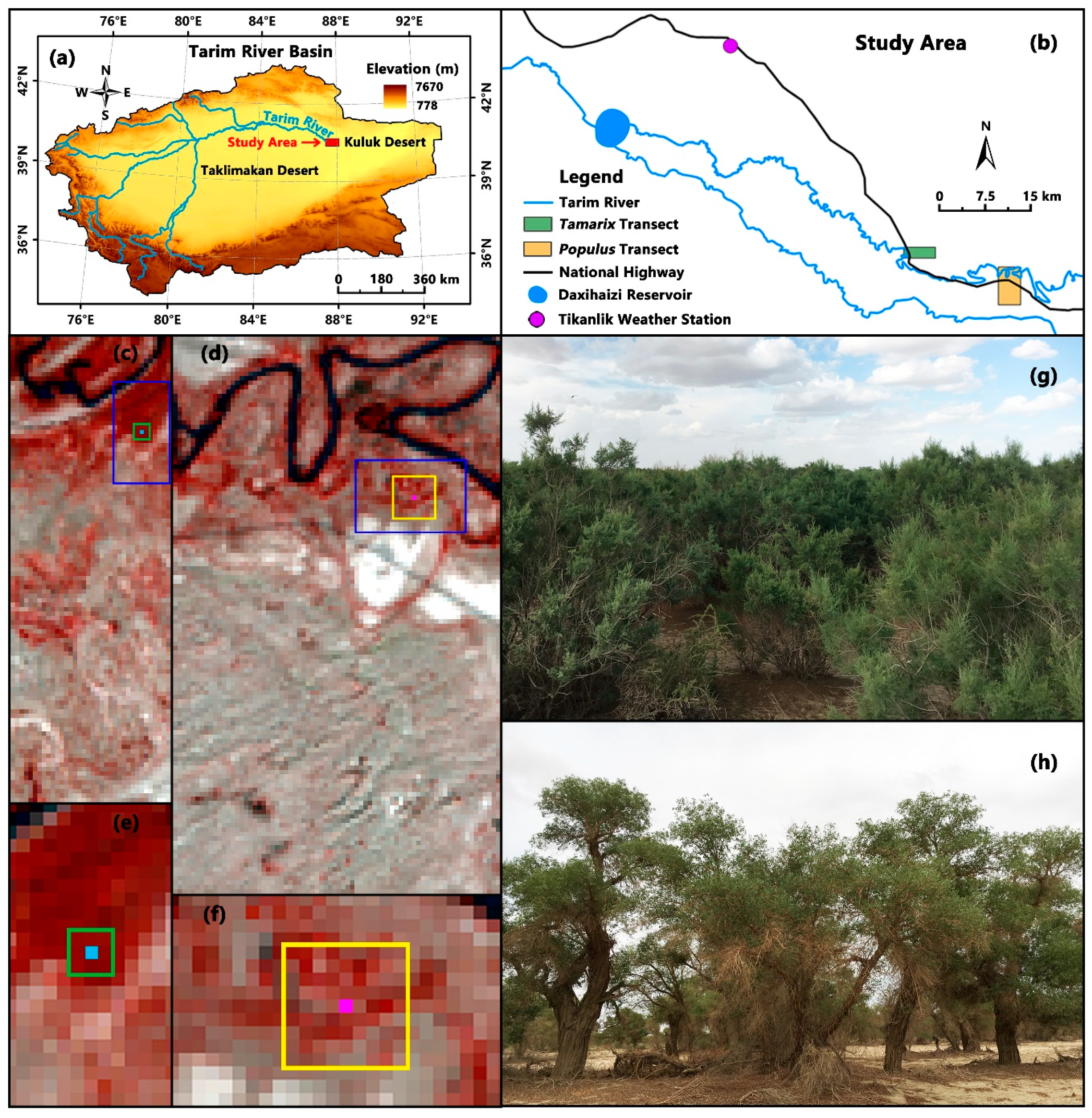
2.2. Site Description and Measurements

The study area is in the Tarim River Basin, which lies in northwestern China and is the largest continental river basin in China with an area of 1.04 × 10⁶ km² [45] (Figure 1). The topography of the study area is relatively flat, and the climate conditions in this region are extremely arid [46]. According to the meteorological records of the Tikanlik Weather Station, the mean annual precipitation was 33.7 mm from 1957 to 2012. The observed maximum annual precipitation was 75.7 mm in 1974 and the minimum annual precipitation was 3.4 mm in 2001. However, the annual potential evapotranspiration was as high as 2000 mm [47,48]. The narrow riparian forest in the lower reaches of the Tarim River distributes within a range of about 3 km from the river channel. Vegetation coverage is less than 0.2 in most of the riparian forest and it generally decreases with increasing distance from the river channel [14]. The vegetation types in this area mainly consist of Tamarix (Tamarix ramosissima) thicket and Populus (Populus euphratica) woodland. Both of the two vegetation communities are phreatophytes that depend almost entirely on groundwater for survival because of the low precipitation [49,50,51].

A typical transect and a typical site were chosen for each vegetation type to conduct this study. The Tamarix transect and the Populus transect covered the Tamarix site and the Populus site, respectively. The two sites were areas with relatively high vegetation coverage and relatively uniform vegetation distribution on the two transects, respectively (Figure 1).

The Tamarix site is located at 87°54′E, 40°27′N, with an altitude of 846 m. The vegetation coverage index was 0.65. The average canopy height was approximately 2 m and the leaf area index measured in July 2013 was 1.15. The dominant species in the site is Tamarix ramosissima, with a small number of herbs (mainly Alhagi sparsifolia and Glycyrrhiza infata) growing under the shrubs. The groundwater table depth fluctuated between 4.4 m and 5.9 m during the observation period, and the soil is mainly silty loam with approximately 20 cm dry sands in the surface layer.

The Populus site is located at 88°1′E, 40°26′N, with an altitude of 844 m. The average canopy height was approximately 10 m. The vegetation coverage index was 0.47 and the leaf area index measured in July 2013 was 0.57. Populus euphratica is the only species at this site. The soil textures at a depth of 0 to 3 m and below 3 m are silty loam and sand, respectively. The groundwater table depth fluctuated between 3.5 m and 6.3 m during the observation period.

The eddy covariance (EC) systems were deployed at the Tamarix site in June 2011 and at the Populus site in June 2013. The EC system was installed at a height of 3.8 m in the Tamarix site and at a height of 15 m in the Populus site (Figure 1). The instruments have been described in detail in [31,49].

2.3. Data and Processing

2.3.1. Daily ET and ET₀ Data

Sensible heat flux (H), latent heat flux (LE), net radiation (R_n), and soil heat flux (G) were measured continuously at each site using the EC system. Data were collected every 30 min during the entire study period. The data processing has been described in [31,49] in detail.

The quality of the measured EC data was evaluated using the energy balance ratio (EBR) method [52]. Due to the sparse and low canopy, the canopy storage heat and the photosynthetic energy consumption were ignored during the analyses, and the EBR was calculated using Equation (1). Our results showed that the EBR was 0.84 for the whole study period. Thus, the measured data satisfied the accuracy requirements for further analysis [52].

$$EBR=\frac{\sum \left(H+LE\right)}{\sum \left(R_n-G\right)}$$

(1)

The energy balance was forced to close by augmenting both H and LE while retaining the observed Bowen ratio [53,54]. In order to ensure accuracy of the analysis, we did not perform gap filling, and only used data with all four components available. Hourly ET (mm h⁻¹) was calculated by the following formula:

$$ET=\frac{L{E}_b}{L\times {\rho }_w}$$

(2)

where $L{E}_b$ is the latent heat (J m⁻² h⁻¹) after energy balance; $L$ is the latent heat of vaporization of water (2.45 kJ g⁻¹); and ${\rho }_w$ is the water density (1 g cm⁻³). The daily ET (mm d⁻¹) was the sum of the hourly ET for one day. In the calculation process, when the hourly ET was negative, it was set to zero.

Daily ET₀ was calculated from the meteorological data with the Penman-Monteith equation [30]. The meteorological data including daily temperature, pressure, wind speed, actual duration of sunshine, and relative humidity were from the Tikanlik Weather Station (Chinese National Weather Station number: 51765). This weather station is the closest one in the China’s National Weather Stations to our study sites with a distance of approximately 30–40 km.

2.3.2. Landsat OLI Imagery and Processing

We used all available Landsat OLI images during the study period. A total of 127 cloud free L1T images with a 30 m pixel resolution were selected and downloaded from the Global Visualization Viewer of the United States Geological Survey (USGS) [55]. The two sites fall in an area overlapped by two adjacent Landsat scenes (paths 141 and 142, row 32), thus resulting in near weekly coverage.

Landsat L1T product processing includes a systematic geometric correction, precision correction assisted by ground control chips, and the use of a digital elevation model (DEM) to correct parallax errors due to terrain relief [56]. Therefore, we did not perform a geometric correction during the pre-processing. The original digital number (DN) values were first converted to absolute at-sensor radiances. The conversion was automatically performed by applying the OLI radiometric calibration parameters available in the ENVI (Environment for Visualizing Images) 5.3.1 software (Exelis Visual Information Solutions, Inc., Boulder, USA) to each band. Afterward, atmospheric correction was performed using its FLAASH (Fast Line-of-Sight Atmospheric Analysis of Spectral Hypercubes) module. This is a MODTRAN (Moderate Resolution Atmospheric Transmission) based algorithm that aims to reduce the extraneous path radiance affecting the pixel’s at-sensor radiometry (i.e., adjacency and haze effects) while modeling the at-surface irradiance. To do so, the mid-latitude summer and sub-Arctic summer atmospheric model was used to define the water vapor amount based on a seasonal-latitude surface temperature model, and the rural aerosol model was selected to define the aerosol type. In addition, the “2-band (K-T)” option was selected for aerosol retrieval in the FLAASH module. After the atmospheric correction, the absolute at-sensor radiances were converted to a surface reflectance value for each pixel.

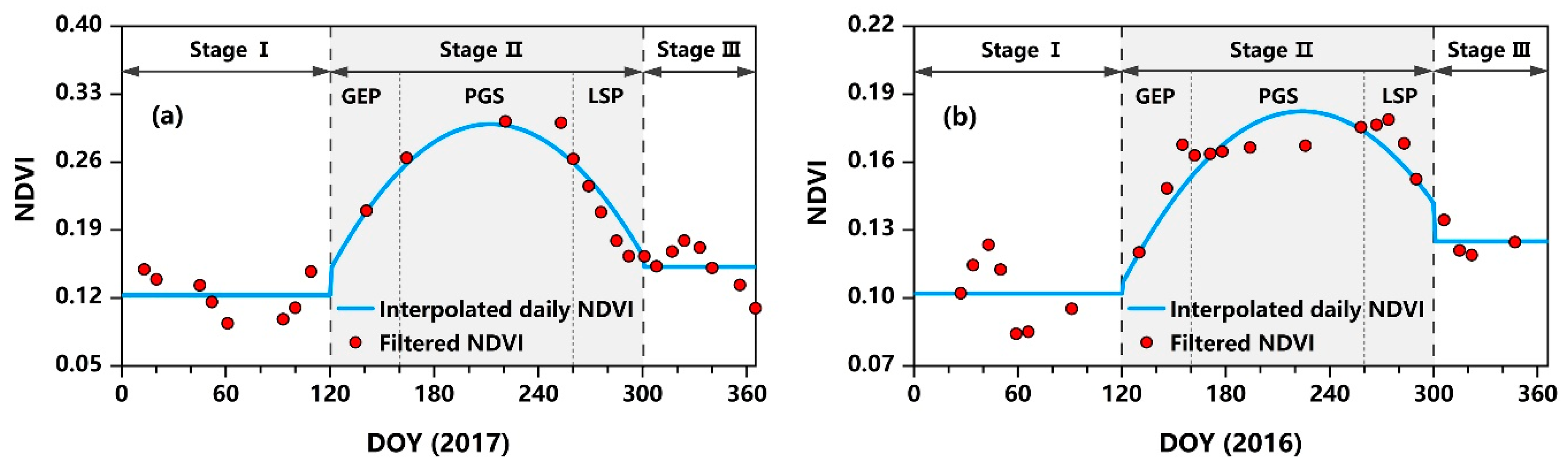
2.3.3. Derivation of NDVI

The NDVI was calculated using the following equation [57] for each image:

$$NDVI=\frac{{\rho }_{NIR}-{\rho }_{Red}}{{\rho }_{NIR}+{\rho }_{Red}}$$

(3)

where ${\rho }_{NIR}$ is the reflectance of near-infrared and ${\rho }_{Red}$ is the reflectance of red. After completing the NDVI calculation for all of the selected Landsat OLI images, we obtained the NDVI time series data. In order to reduce the perturbations from varying atmospheric conditions and sun-sensor-surface viewing geometries, the NDVI time series data need to be smoothed before being used [58,59]. In the present study, the Savitzky-Golay filter [60] was used to smooth the NDVI time series due to its better performance in arid ecosystems of northwestern China [61]. Two parameters must be determined when the Savitzky-Golay filter is applied to NDVI time series smoothing. The first parameter is the half-width of the smoothing window. Usually, a larger value of it produces a smoother result at the expense of flattening sharp peaks. The second parameter specifies the degree of the smoothing polynomial, which is typically set in a range from 2 to 4. A smaller value will produce a smoother result, but may introduce bias; a higher value will reduce the filter bias, but may “over fit” the data and give a noisier result [62]. In this study, we used the value of three for both parameters according to the NDVI observations.

In order to comprehensively compare the simulation capabilities of CVTM and SVTM using more observed daily ET data at the site scale and to perform comparison of the annual ET estimation at regional scale, a daily-basis NDVI time series for 2017 of the Tamarix transect and for 2016 of the Populus transect were needed. Therefore, we interpolated the two NDVI time series in a way that treated each pixel individually. In the process of NDVI time series interpolation, we divided the whole year into three stages according to local phenology and the filtered NDVI time series: Stage I was from the beginning of the year to the beginning of the growing season (DOY 1 to DOY 120); Stage II was the growing season (DOY 121 to DOY 300); and Stage III was from the end of the growing season to the end of the year (DOY 301 to DOY 365 or DOY 366). Stage II was further divided into the germination and leaf expansion period (GEP, DOY 121 to DOY 160), the peak growing season (PGS, DOY 161 to DOY 260), and the leaf senescence period (LSP, DOY 261 to DOY 300) [49]. For Stage II, a quadratic function was used to fit the filtered NDVI data points with DOY, and daily NDVI could be simulated using the fitted quadratic function. For Stage I and Stage III, the daily NDVI was assigned by the corresponding average values respectively (Figure 2). In order to ensure that the fitted quadratic curve of Stage II was as continuous as possible with the end point of Stage I and the starting point of Stage III, during the fitting process, the quadratic function was forced to pass through the first and last data points of Stage II.

Finally, we extracted the NDVI values over the footprint area (9 pixels, Figure 1e) around the Tamarix flux tower and over the footprint area (81 pixels, Figure 1f) around the Populus flux tower, respectively. The extraction was performed for both the filtered NDVI time series and the interpolated NDVI time series, and the extracted NDVI values were spatially averaged for analyses at the site scale. Figure 2 shows the comparison between the filtered NDVI and the interpolated daily NDVI throughout 2017 for the Tamarix site and throughout 2016 for the Populus site. In addition, the interpolated NDVI time series values for pixels covering the Tamarix transect (3446 pixels) and covering the Populus transect (7984 pixels) were extracted for the annual ET estimation of each transect.

2.3.4. Statistical Analyses

Statistical analyses were performed using the software OriginPro 2016 (OriginLab Corporation, Northampton, MA, USA). Nonlinear regression equations were fitted to data points by the least squares method and goodness of fit is reported as the determination coefficient (R²), reduced chi-sqr values, and P-values for the regression coefficient. The reduced chi-sqr value equals the sum of the residuals squared divided by the degrees of freedom. Smaller reduced chi-sqr values represent a better curve fit. P < 0.001 was considered to be statistically significant.

2.4. Evaluation of Model Performance

The simulated daily ET values were compared with the observed values by the flux tower at each site. Model performance was evaluated with metrics that included determination coefficient (R², Equation (4)), root mean square error (RMSE, Equation (5)), Nash-Sutcliffe efficiency (NSE, Equation (6)), mean error (ME, Equation (7)) and maximum error (MaxError, Equation (8)). These metrics are the most widely used by researchers to evaluate the performance of ET models [63,64].

$$R^2=\frac{{\left[{{\displaystyle \sum }}_{i=1}^n\left(E{T}_{s,i}-{\phi }_0\right)\left(E{T}_{o,i}-{\mu }_0\right)\right]}^2}{{{\displaystyle \sum }}_{i=1}^n{\left(E{T}_{s,i}-{\phi }_0\right)}^2{{\displaystyle \sum }}_{i=1}^n{\left(E{T}_{o,i}-{\mu }_0\right)}^2}$$

(4)

$$RMSE=\sqrt{\frac{{{\displaystyle \sum }}_{i=1}^n{\left(E{T}_{s,i}-E{T}_{o,i}\right)}^2}{n}}$$

(5)

$$NSE=1-\frac{{{\displaystyle \sum }}_{i=1}^n{\left(E{T}_{s,i}-E{T}_{o,i}\right)}^2}{{{\displaystyle \sum }}_{i=1}^n{\left(E{T}_{o,i}-{\mu }_0\right)}^2}$$

(6)

$$ME=\frac{1}{n}{\displaystyle \sum }_{i=1}^n\left(E{T}_{s,i}-E{T}_{o,i}\right)$$

(7)

$$MaxError=\max \left|E{T}_{s,i}-E{T}_{o,i}\right|$$

(8)

where $n$ is the total number of observation days; $E{T}_{s,i}$ is the simulated value during day I, $E{T}_{o,i}$ is the observed value during day I, and ${\mu }_0$ and ${\phi }_0$ are the mean of the observed and simulated values, respectively.

3. Results

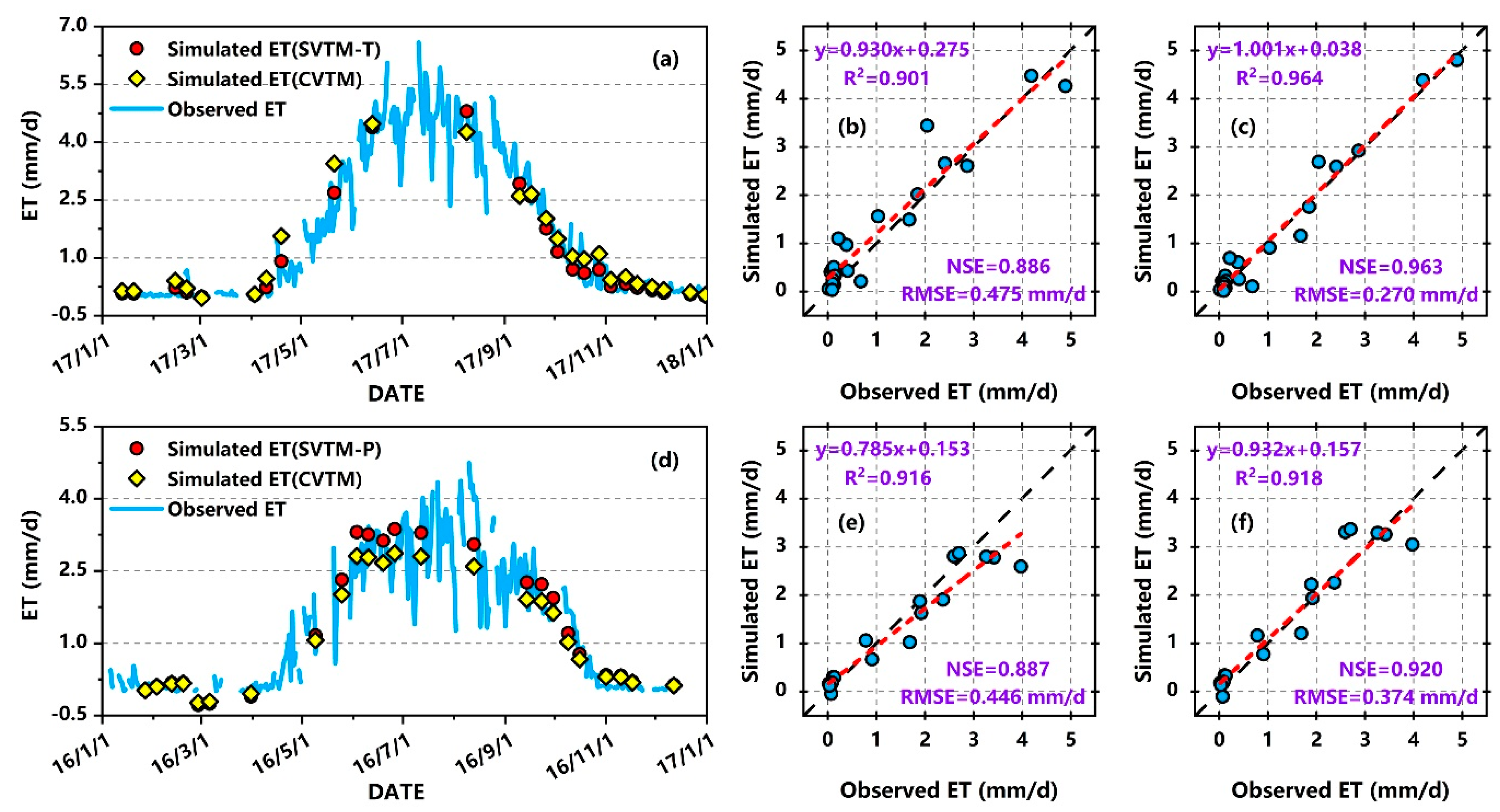
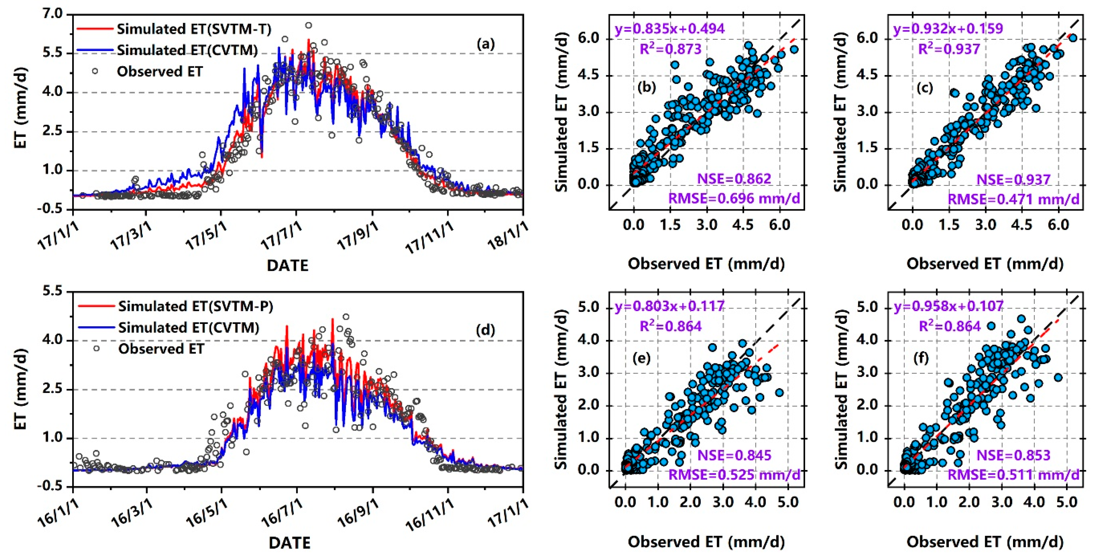
3.1. Calibration and Validation of CVTM and SVTM

Table 2. Calibration results of CVTM, SVTM-T and SVTM-P.

Models	a	b	c	R2	Reduced chi-sqr
CVTM	2.364	11.681	1.597	0.809	0.492
SVTM-T	17.993	0.221	0.374	0.862	0.433
SVTM-P	2.652	9.598	1.611	0.845	0.312

shows the calibration results for the CVTM, SVTM-T, and SVTM-P. The minimum determination coefficient (R²) in all models was 0.809, and the maximum reduced chi-sqr value was 0.492, indicating successful calibrations for all models. Notably, the parameters varied greatly between the CVTM and the SVTM-T, and the parameters of the CVTM were closer to that of SVTM-P.

The calibrated CVTM, SVTM-T, and SVTM-P were then validated using the validation dataset of the Tamarix site and Populus site. Figure 3 shows the time series and scatter plots of the observed and simulated daily ET at the Tamarix site (Figure 3a–c) and at the Populus site (Figure 3d–f). The time courses of daily ET estimated by CVTM and SVTM-T for the Tamarix site (Figure 3a) and estimated by CVTM and SVTM-P for the Populus site (Figure 3d) satisfactorily reproduced the trend of the observations. Scatter plots of observed and simulated daily ET suggested overall, acceptable agreement, when the CVTM (Figure 3b) and the SVTM-T (Figure 3c) were used for the Tamarix site and when the CVTM (Figure 3e) and the SVTM-P (Figure 3f) were used for the Populus site.

3.2. Comparison of Estimates from CVTM and SVTM

3.2.1. Estimation Accuracy at Site Scale

First, the validation results of CVTM and SVTM-T for the Tamarix site, and CVTM and SVTM-P for the Populus site (Figure 3) were compared. For the Tamarix site, the SVTM-T showed a higher determination coefficient (R² = 0.964), NSE (0.963) and lower RMSE (0.270 mm/d) (Figure 3c), followed by the CVTM (R² = 0.901, NSE = 0.886, and RMSE = 0.475 mm/d) (Figure 3b). For the Populus site, the SVTM-P had better performance (R² = 0.918, NSE = 0.920, and RMSE = 0.374 mm/d) (Figure 3f) than the CVTM (R² = 0.916, NSE = 0.887, and RMSE = 0.446 mm/d) (Figure 3e). However, the CVTM slightly underestimated the high values for the Populus site.

Figure 4 depicts the comparison between the observed and simulated daily ET throughout 2017 for the Tamarix site and throughout 2016 for the Populus site. Similarly, good agreements were found between the observed and simulated daily ET values for the Tamarix site (Figure 4a−c) and for the Populus site (Figure 4d−f) with roughly consistent time courses and the R² values ranging from 0.864 to 0.937. There were some discrepancies in the performance between the CVTM (Figure 4b) and the SVTM-T (Figure 4c) for the Tamarix site, and in the performance between the CVTM (Figure 4e) and the SVTM-P (Figure 4f) for the Populus site. Overall, the SVTM-T and the SVTM-P had better performance with a higher determination coefficient (R²), NSE, and relatively lower RMSE for both sites, and the CVTM showed relatively poor performance and tended to underestimate at higher values of daily ET and slightly overestimate at the low daily ET range. For the Tamarix site, the CVTM overestimated the daily ET values at the beginning of the growing season (Figure 4a). For the Populus site, the CVTM underestimated the daily ET values for the peak growing season (PGS) (Figure 4d).

Table 3. Comparison of mean error (ME) and MaxError for the CVTM, SVTM-T and the SVTM-P.

Sites	Dataset	N	ME (mm/d)			MaxError (mm/d)
			CVTM	SVTM-T	SVTM-P	CVTM	SVTM-T	SVTM-P
Tamarix site	Validation Data	21	0.197	0.040		1.399	0.646
	Throughout 2017	294	0.177	0.029		3.235	2.103
Populus site	Validation Data	18	−0.158		0.059	1.380		0.922
	Throughout 2016	264	−0.163		0.047	2.336		1.870

shows the comparison of the mean error (ME) and maximum error (MaxError) between the simulated daily ET from CVTM, SVTM-T, SVTM-P, and the observed values. Results showed that both ME and MaxError for SVTM-T and SVTM-P were lower than that for CVTM, indicating the better performance of SVTM-T and SVTM-P. Interestingly, for the ME, the SVTM-T and SVTM-P showed a small positive bias for both sites, but it was different for the CVTM, which manifested a small positive bias for the Tamarix site and a small negative bias for the Populus site.

Table 4. Comparisons of observed and simulated ET from CVTM and SVTM-T for the Tamarix site, and from CVTM and SVTM-P for the Populus site at monthly and yearly scales.

Month	ET for Tamarix Site				ET for Populus Site
	N	Observed (mm)	CVTM (mm)	SVTM-T (mm)	N	Observed (mm)	CVTM (mm)	SVTM-P (mm)
January	11	0.51	1.56	0.82	20	3.48	0.54	0.49
February	23	2.43	6.03	3.16	14	0.64	0.80	0.73
March	19	1.16	11.63	6.10	13	1.51	2.08	1.90
April	24	11.71	27.66	15.01	28	9.79	7.11	6.59
May	30	64.07	98.12	74.14	14	23.06	16.03	17.83
June	27	113.23	118.79	115.66	29	82.28	79.87	93.26
July	29	138.30	122.31	133.59	27	84.13	80.39	95.47
August	28	117.74	103.23	112.94	26	77.09	60.80	72.52
September	30	83.38	82.53	80.20	30	64.08	55.15	65.31
October	28	24.19	32.63	24.68	26	25.38	20.64	23.91
November	22	5.67	8.50	5.08	24	2.06	6.24	6.96
December	23	3.39	4.82	2.88	13	0.73	1.54	1.71
Average	25	47.15	51.48	47.85	22	31.18	27.60	32.22
Total	294	565.78	617.80	574.25	264	374.22	331.17	386.68
Residual Error			52.02 (9.19%)	8.47 (1.50%)			−43.04 (−11.50%)	12.47 (3.33%)

shows the comparison of the total amount of ET on the monthly and yearly scales. On the monthly scale, compared with the CVTM, the SVTM-T and SVTM-P had better performance, with lower residual errors of monthly average ET values. The CVTM obviously overestimated ET of the Tamarix site from March to May, and underestimated ET of the Populus site from June to September. On a yearly scale, the CVTM had larger residual errors than the SVTM-T and SVTM-P. The residual errors of the simulated annual ET from the SVTM-T and SVTM-P were 1.50% and 3.33%, respectively, while that from the CVTM were 9.19% and −11.50% for the Tamarix site and the Populus site, respectively.

These results are complementary and indicate that distinguishing vegetation types can improve the accuracy of ET estimation at the site scale, and that the combination of datasets from different vegetation types introduced obvious errors at the beginning of the growing season of Tamarix ramosissima and at the peak growing season of Populus euphratica.

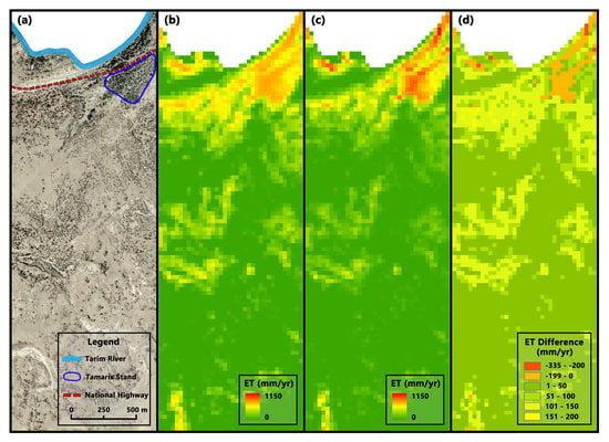
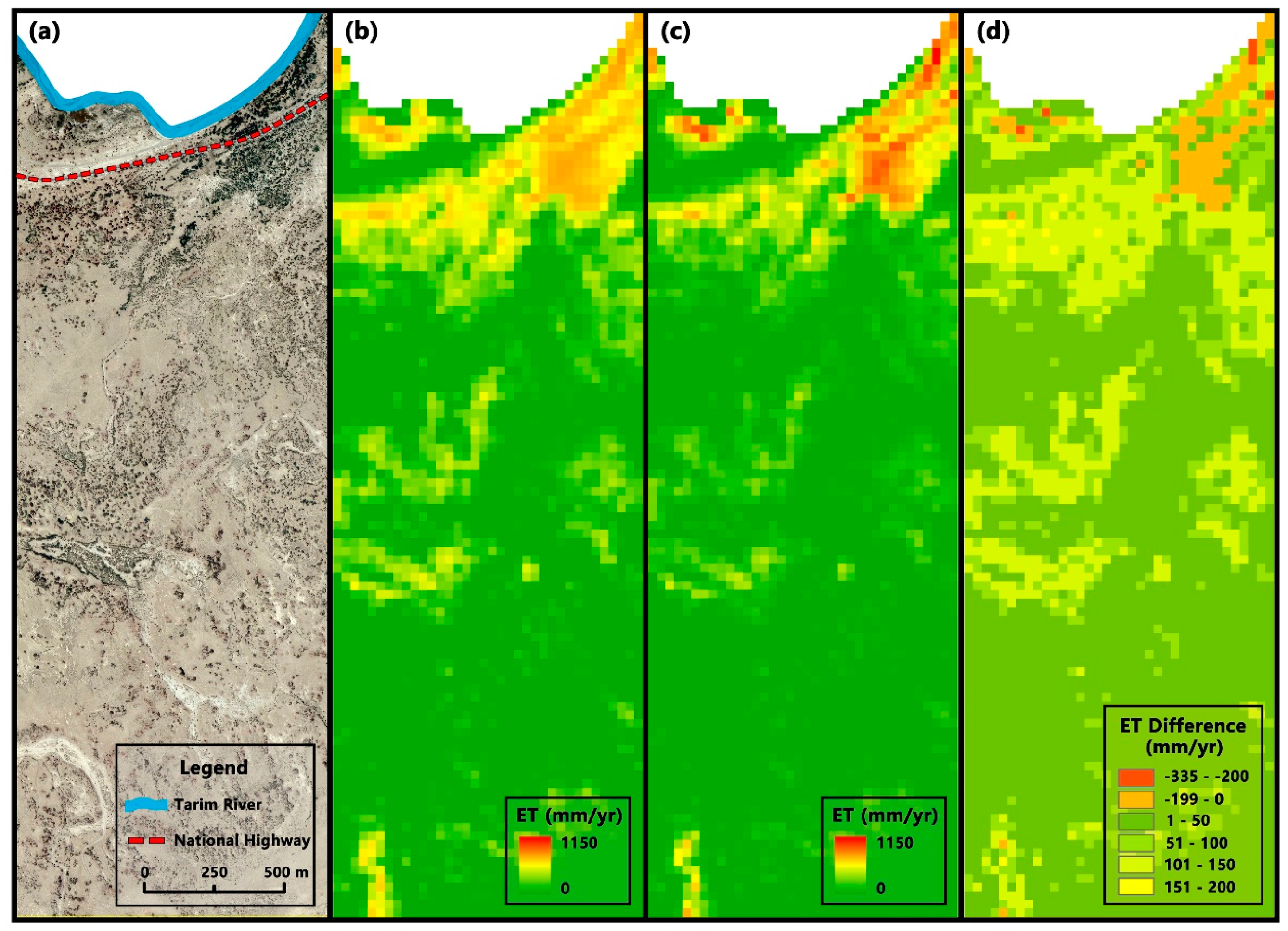
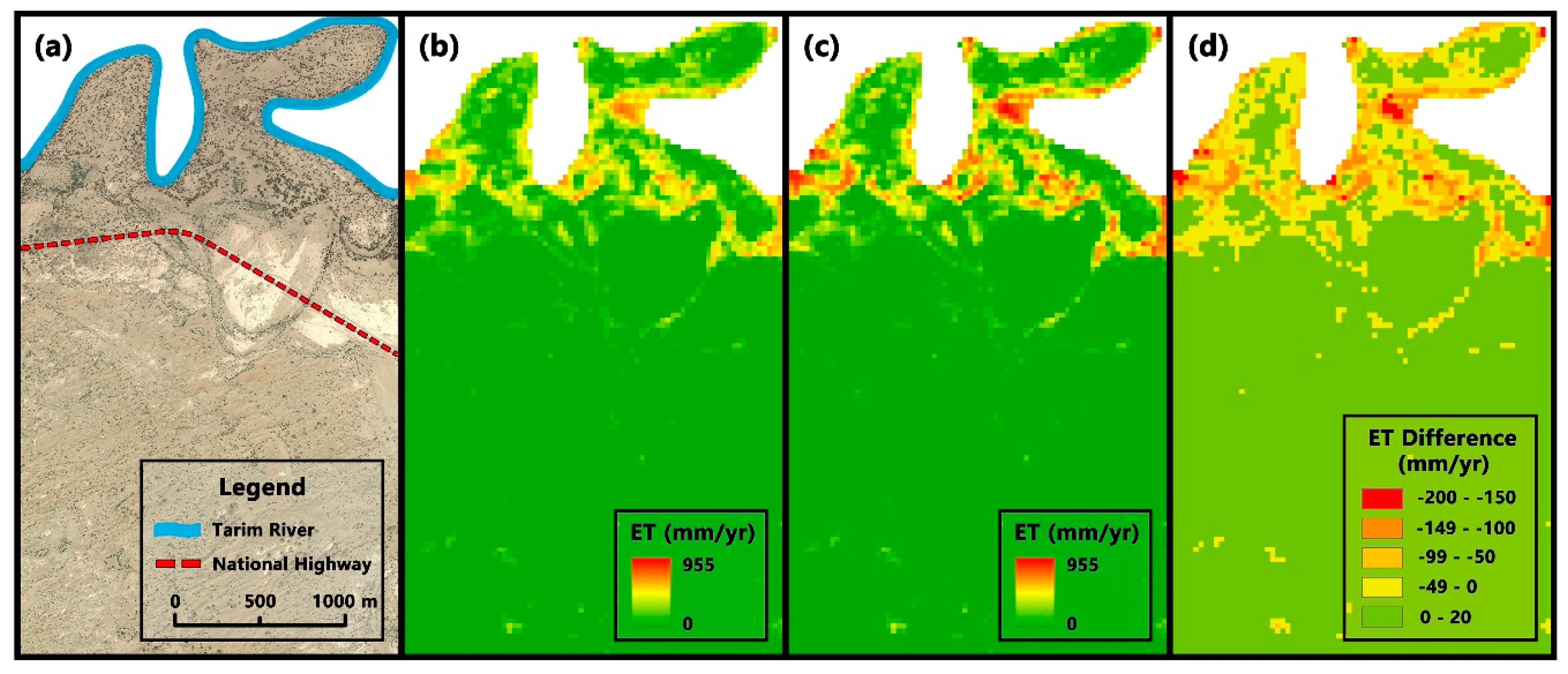
3.2.2. Differences in Regional Scale

Figure 5 and Figure 6 show the difference in annual ET estimation between CVTM and SVTM for the Tamarix transect and the Populus transect, respectively. Overall, the annual ET estimated by CVTM and SVTM-T for the Tamarix transect (Figure 5b,c) and estimated by CVTM and SVTM-P for the Populus transect (Figure 6b,c) showed similar spatial patterns. The annual ET decreased with decreasing vegetation coverage.

However, substantial difference in annual ET estimation was revealed between CVTM and SVTM for both transects (Figure 5d and Figure 6d). For pixels over the Tamarix transect (Figure 5d), the difference in annual ET (CVTM−SVTM-T) ranged from −333.94 to 160.31 mm yr⁻¹. For pixels over the Populus transect (Figure 6d), the difference in annual ET (CVTM−SVTM-P) ranged from −200.42 to 11.87 mm yr⁻¹. For pixels in the bare soil area, the annual ET difference of both the Tamarix transect and the Populus transect were positive, indicating that CVTM overestimated annual ET of bare soil area when compared with the SVTM. For pixels in the vegetation area, the higher the vegetation coverage, the greater the difference in annual ET between CVTM and SVTM. The annual ET difference for pixels in the vegetation area of the Populus transect was negative, suggesting that CVTM underestimated annual ET in the vegetation area of the Populus transect compared with SVTM-P. Notably, for pixels in the vegetation area of the Tamarix transect, the annual ET difference was negative for pixels in the upper right corner with higher vegetation coverage, while positive for the others with lower vegetation coverage. These characteristics of the annual ET difference for the vegetation area of the Tamarix transect suggest that compared with SVTM-T, CVTM overestimated annual ET in area with lower vegetation coverage and underestimated annual ET in area with higher vegetation coverage. These results indicate that for the area with higher vegetation coverage of Tamarix ramosissima, the underestimation of high daily ET values by CVTM had greater impact on the annual ET than the overestimation of low daily ET values by CVTM (Figure 4b), and that was opposite for the area with lower vegetation coverage.

These results revealed that the empirical daily ET model built on the site scale played the dominant role in the accuracy of ET estimation, and that a minor difference in daily ET estimation at the site scale can lead to a large difference in annual ET estimation at regional scale.

4. Discussion

4.1. Effects of Distinguishing Vegetation Types

The estimation accuracy of ET was improved by distinguishing vegetation types at the site scale in our study. The SVTM-T and SVTM-P achieved higher accuracy for the ET estimation of Tamarix ramosissima and Populus euphratica, respectively, than the CVTM at the daily, monthly, and yearly scales. Similarly, Nagler et al. [7] constructed empirical remotely sensed ET model using datasets from five vegetation types (cottonwood, mesquite, saltcedar, giant sacaton, and arrowweed) over the western U.S. rivers, and then estimated ET for individual vegetation type using the constructed ET model. They reported that the simulated and observed average daily ET during the growing season were within 25% of the 1:1 line for all vegetation types, except for the arrowweed, for which simulated average daily ET was 40% higher than the observed values. Nouri et al. [43] compared the ET estimation of the Nagler model with a detailed soil water balance analysis in an urban parkland of Australia, which was fully covered by kikuyu turf grasses and more than 60 species of trees and shrubs. They noted that the estimates of the Nagler model was not accurate at the monthly scale, but errors were cancelled out to give good agreement on an annual time step. Moreover, compared with the validation results of SVTM in this study, the empirical ET models constructed based on combined vegetation types had relatively poor validation accuracy. For example, Nagler et al. [10] reported an error or uncertainty of about 20% in the average daily ET (6.2 mm d⁻¹ with RMSE = 1.2 mm d⁻¹); Nagler et al. [11] reported that the average error of annual ET was 5.5%, ranging from 2.9% to 9.3% across sites; Glenn et al. [13] reported validation results with R² = 0.72. Nevertheless, Oliveira et al. [44] recalibrated the Nagler model using two year of data from a cerrado woodland site (arborous cover is about 50–70%) in South America and validated it using another year of data. They reported that the recalibrated model showed significant agreement with the observed ET at the daily, monthly, and yearly scale. Therefore, combined vegetation types produced biased ET estimation.

The CVTM overestimated ET of 2017 about 9.19% for Tamarix ramosissima and underestimated ET of 2016 about 11.50% for Populus euphratica at the site scale, mainly at the beginning of the growing season of Tamarix ramosissima and at the peak growing season of Populus euphratica, respectively. Furthermore, for annual ET at regional scale, there was considerable difference between CVTM and SVTM. Compared with SVTM-P, the CVTM underestimated annual ET for vegetation areas of the Populus transect. Compared with SVTM-T, the CVTM overestimated annual ET in areas with lower vegetation coverage and underestimated annual ET in areas with higher vegetation coverage for vegetation areas of the Tamarix transect. These unquestionably resulted from the model parameters calibrated using the combined datasets from different vegetation types, which led to biased daily ET estimation at the site scale and ultimately exaggerated for annual ET estimation at the regional scale. In addition, Nagler et al. [7] estimated ET of five vegetation types with different water-consumption characteristics using a model based on combined vegetation types. Their estimation results indicated that the average daily ET of cottonwood with high water-consumption was underestimated, and that of arrowweed with low water-consumption was obviously overestimated. Therefore, when using these empirical remotely sensed ET models to estimate regional scale ET for highly heterogeneous riparian zones on a large time scale, the CVTM may underestimate ET for high water-consumption vegetation (for example, Populus euphratica) and tend to overestimate ET for low water-consumption vegetation (for example, Tamarix ramosissima).

After distinguishing vegetation types, the SVTM-T and the SVTM-P obtained very high estimation accuracy at the site scale. However, both the mean errors (ME) of daily ET (Table 3) and the annual ET from SVTM-T and SVTM-P (Table 4) showed positive bias. Likewise, Nagler et al. [11] reported an average bias of 5.5% (ranging from 2.9% to 9.3% across sites) for annual ET estimation. Nouri et al. [43] reported that the annual ET estimated by the Nagler model had a bias of 4 mm yr⁻¹ compared with a detailed soil water balance analysis. Thus, this may be a systematic bias determined by the structure of the Nagler model and needs to be further tested.

4.2. Feasibility of the Application of SVTM

Essentially, the Nagler model is a modification of the crop coefficient method [6]. The crop coefficient approach assumes that the plant is growing under unstressed conditions [29]. In the Nagler model, crop coefficient was replaced by a satellite-derived VI that provides information about the actual status of the canopy at the time of measurement. VI-based methods cannot detect early signs of plant moisture stress [29], which added scatter and uncertainty into the ET estimation [6]. In arid ecosystems, plant transpiration dominates ET, with weak and negligible soil evaporation due to the scant rainfall [6,49]. Moreover, the phreatophytes mainly obtain water from the capillary fringe and groundwater [50,51], thus they have a relatively constant transpiration rate that related to groundwater table depth and salinity [6]. Therefore, these features in arid ecosystems provide good conditions for the application of these empirical remotely sensed ET models. In this study, the very high estimation accuracy of the SVTM-T and SVTM-P at the site scale seems to be related to the suitable hydrological conditions of the two vegetation types in the study area. Yuan et al. [31] reported that the groundwater table depth is a decisive indicator of hydrological conditions in the study area. According to the reported thresholds in [65], the groundwater table depth during the study period (see Section 2.2) is suitable for the growth of vegetation in the lower reaches of the Tarim River.

When the SVTM is applied to other arid regions, the necessary prerequisite is to distinguish different vegetation types. Vegetation in arid regions is relatively sparse and their spatial structure is usually simple. As a result, it is easy and feasible to distinguish different vegetation types by using remote sensing images [41,66,67], and some effective classification methods with high accuracy have been proposed [68,69]. Therefore, the estimation method based on specific vegetation type proposed in this study is feasible in practical applications. It should be noted that it is also necessary to recalibrate the empirical parameters of these remotely sensed ET models for the specific vegetation type of concern.

The number of remote sensing images available is crucial to the application of these empirical remotely sensed ET models because it is the basis for achieving high-quality NDVI time series data. Ruhoff et al. [70] reported that the vegetation index (NDVI) was the most important item among the main inputs for ET estimation in the SEBAL algorithm. In this study, the Nagler model was used to estimate ET based on the meteorological data and the vegetation indices (NDVI), which were derived from Landsat OLI images. The Nagler model is an empirical ET model, which was constructed by directly relating ET to vegetation indices (VIs) and meteorological data, and thus it is different from the SEBAL algorithm that estimates ET using the energy balance equation. In addition, although we interpolated the NDVI time series during the comparison between CVTM and SVTM, we still obtained a satisfactory ET estimation (Figure 4). This may be related to the NDVI observations we used for interpolation. Since the study area is located in the overlap of two adjacent images, we had at least one NDVI observation every month throughout the year (Figure 2). Therefore, the number of images available seemed to have little impact on the ET estimation in this study. Nevertheless, the 16 day revisit cycle of the Landsat series satellites (e.g., TM/ETM+/OLI with 30 m spatial resolution) and frequent cloud contamination in some regions limit their application for frequent ET estimation using these empirical remotely sensed ET models [7]. On the other hand, MODIS (MODerate-resolution Imaging Spectroradiometer) has a high temporal resolution (1 day) with the spatial resolutions of 250 m, 500 m, and 1000 m. However, it is difficult to capture spatial details necessary for monitoring land cover and ecosystem changes in heterogeneous areas, especially for narrow riparian corridors [71]. Hence, in the process of ET estimation, appropriate spatial- and temporal-resolution NDVI data should be selected according to the research needs.

5. Conclusions

In this study, using the Nagler model [11] and the datasets from two typical vegetation types (Tamarix ramosissima and Populus euphratica) in arid ecosystems of northwestern China, we investigated the effects of distinguishing vegetation types on the estimates of remotely sensed ET at site and regional scales.

By distinguishing vegetation types, the accuracy of ET estimation was improved. The combined vegetation types introduced errors in the ET estimation and had a great influence on the estimation accuracy of annual ET. Furthermore, CVTM and SVTM had a substantial difference in annual ET estimation at the regional scale, and the higher the vegetation coverage, the greater the difference in annual ET between the CVTM and SVTM. In addition, the SVTM-T and SVTM-P had very high estimation accuracy of daily, monthly, and yearly ET at the site scale, therefore, the calibration parameters for SVTM-T and SVTM-P in Table 2 are recommended for the ET estimation of Tamarix ramosissima and Populus euphratica in arid ecosystems of northwestern China. At the same time, the estimation method based on specific vegetation type proposed in this study is feasible in practical applications in other arid ecosystems.

Further study is recommended to investigate the impacts of distinguishing vegetation types on the accuracy of ET estimation at the site scale using data from more sites under different vegetation types and to indirectly evaluate the regional scale ET estimation with the aid of the groundwater model using the measured groundwater level [72,73].

References

1. Chen, Y.; Xia, J.; Liang, S.; Feng, J.; Fisher, J.B.; Li, X.; Li, X.; Liu, S.; Ma, Z.; Miyata, A.; et al. Comparison of satellite-based evapotranspiration models over terrestrial ecosystems in China. Remote Sens. Environ. 2014, 140, 279–293. [Google Scholar] [CrossRef]
2. Wang, S.; Pan, M.; Mu, Q.; Shi, X.; Mao, J.; Brümmer, C.; Jassal, R.S.; Krishnan, P.; Li, J.; Black, T.A. Comparing Evapotranspiration from Eddy Covariance Measurements, Water Budgets, Remote Sensing, and Land Surface Models over Canada. J. Hydrometeorol. 2015, 16, 1540–1560. [Google Scholar] [CrossRef]
3. McCabe, M.F.; Wood, E.F. Scale influences on the remote estimation of evapotranspiration using multiple satellite sensors. Remote Sens. Environ. 2006, 105, 271–285. [Google Scholar] [CrossRef]
4. Cleverly, J.R.; Dahm, C.N.; Thibault, J.R.; Mcdonnell, D.E.; Coonrod, J.E.A. Riparian ecohydrology: Regulation of water flux from the ground to the atmosphere in the Middle Rio Grande, New Mexico. Hydrol. Process. 2006, 20, 3207–3225. [Google Scholar] [CrossRef]
5. Falkenmark, M.; Rockström, J. Balancing Water for Humans and Nature: The New Approach in Ecohydrology; Earthscan: London, UK, 2004. [Google Scholar]
6. Nagler, P.L.; Cleverly, J.; Glenn, E.; Lampkin, D.; Huete, A.; Wan, Z. Predicting riparian evapotranspiration from MODIS vegetation indices and meteorological data. Remote Sens. Environ. 2005, 94, 17–30. [Google Scholar] [CrossRef]
7. Nagler, P.L.; Scott, R.L.; Westenburg, C.; Cleverly, J.R.; Glenn, E.P.; Huete, A.R. Evapotranspiration on western US rivers estimated using the Enhanced Vegetation Index from MODIS and data from eddy covariance and Bowen ratio flux towers. Remote Sens. Environ. 2005, 97, 337–351. [Google Scholar] [CrossRef]
8. Groeneveld, D.P.; Baugh, W.M.; Sanderson, J.S.; Cooper, D.J. Annual groundwater evapotranspiration mapped from single satellite scenes. J. Hydrol. 2007, 344, 146–156. [Google Scholar] [CrossRef]
9. Scott, R.L.; Cable, W.L.; Huxman, T.E.; Nagler, P.L.; Hernandez, M.; Goodrich, D.C. Multiyear riparian evapotranspiration and groundwater use for a semiarid watershed. J. Arid Environ. 2008, 72, 1232–1246. [Google Scholar] [CrossRef]
10. Nagler, P.L.; Morino, K.; Murray, R.S.; Osterberg, J.; Glenn, E.P. An Empirical Algorithm for Estimating Agricultural and Riparian Evapotranspiration Using MODIS Enhanced Vegetation Index and Ground Measurements of ET. I. Description of Method. Remote Sens. 2009, 1, 1273–1297. [Google Scholar] [CrossRef]
11. Nagler, P.L.; Glenn, E.P.; Nguyen, U.; Scott, R.L.; Doody, T. Estimating riparian and agricultural actual evapotranspiration by reference evapotranspiration and MODIS enhanced vegetation index. Remote Sens. 2013, 5, 3849–3871. [Google Scholar] [CrossRef]
12. Bunting, D.P.; Kurc, S.A.; Glenn, E.P.; Nagler, P.L.; Scott, R.L. Insights for empirically modeling evapotranspiration influenced by riparian and upland vegetation in semiarid regions. J. Arid Environ. 2014, 111, 42–52. [Google Scholar] [CrossRef]
13. Glenn, E.P.; Scott, R.L.; Nguyen, U.; Nagler, P.L. Wide-area ratios of evapotranspiration to precipitation in monsoon-dependent semiarid vegetation communities. J. Arid Environ. 2015, 117, 84–95. [Google Scholar] [CrossRef]
14. Yuan, G.; Zhu, X.; Tang, X.; Du, T.; Yi, X. A Species-Specific and spatially-Explicit Model for Estimating Vegetation Water Requirements in Desert Riparian Forest Zones. Water Resour. Manag. 2016, 30, 1–19. [Google Scholar] [CrossRef]
15. Groeneveld, D.P. Remotely-sensed groundwater evapotranspiration from alkali scrub affected by declining water table. J. Hydrol. 2008, 358, 294–303. [Google Scholar] [CrossRef]
16. Murray, R.S.; Nagler, P.L.; Morino, K.; Glenn, E.P. An Empirical Algorithm for Estimating Agricultural and Riparian Evapotranspiration Using MODIS Enhanced Vegetation Index and Ground Measurements of ET. II. Application to the Lower Colorado River, U.S. Remote Sens. 2009, 1, 1125–1138. [Google Scholar] [CrossRef]
17. Nagler, P.L.; Pearlstein, S.; Glenn, E.P.; Brown, T.B.; Bateman, H.L.; Bean, D.W.; Hultine, K.R. Rapid dispersal of saltcedar (Tamarix spp.) biocontrol beetles (Diorhabda carinulata) on a desert river detected by phenocams, MODIS imagery and ground observations. Remote Sens. Environ. 2014, 140, 206–219. [Google Scholar] [CrossRef]
18. Nagler, P.L.; Doody, T.M.; Glenn, E.P.; Jarchow, C.J.; Barreto-Muñoz, A.; Didan, K. Wide-area estimates of evapotranspiration by red gum (Eucalyptus camaldulensis) and associated vegetation in the Murray–Darling River Basin, Australia. Hydrol. Process. 2016, 30, 1376–1387. [Google Scholar] [CrossRef]
19. Tillman, F.D.; Wiele, S.M.; Pool, D.R. A comparison of estimates of basin-scale soil-moisture evapotranspiration and estimates of riparian groundwater evapotranspiration with implications for water budgets in the Verde Valley, Central Arizona, USA. J. Arid Environ. 2016, 124, 278–291. [Google Scholar] [CrossRef]
20. Jarchow, C.J.; Nagler, P.L.; Glenn, E.P.; Ramírez-Hernández, J.; Rodríguez-Burgueño, J.E. Evapotranspiration by remote sensing: An analysis of the Colorado River Delta before and after the Minute 319 pulse flow to Mexico. Ecol. Eng. 2017, 106, 725–732. [Google Scholar] [CrossRef]
21. Khand, K.; Taghvaeian, S.; Hassan-Esfahani, L. Mapping Annual Riparian Water Use Based on the Single-Satellite-Scene Approach. Remote Sens. 2017, 9, 832. [Google Scholar] [CrossRef]
22. Knipper, K.; Hogue, T.; Scott, R.; Franz, K. Evapotranspiration Estimates Derived Using Multi-Platform Remote Sensing in a Semiarid Region. Remote Sens. 2017, 9, 184. [Google Scholar] [CrossRef]
23. Shanafield, M.; Gutiérrez-Jurado, H.; Rodríguez-Burgueño, J.E.; Ramírez-Hernández, J.; Jarchow, C.J.; Nagler, P.L. Short- and long-term evapotranspiration rates at ecological restoration sites along a large river receiving rare flow events. Hydrol. Process. 2017, 31, 4328–4337. [Google Scholar] [CrossRef]
24. Nagler, P.L.; Morino, K.; Didan, K.; Erker, J.; Osterberg, J.; Hultine, K.R.; Glenn, E.P. Wide-area estimates of saltcedar (Tamarix spp.) evapotranspiration on the lower Colorado River measured by heat balance and remote sensing methods. Ecohydrology 2009, 2, 18–33. [Google Scholar] [CrossRef]
25. Nagler, P.L.; Nguyen, U.; Bateman, H.L.; Jarchow, C.J.; Glenn, E.P.; Waugh, W.J.; van Riper, C., III. Northern tamarisk beetle (Diorhabda carinulata) and tamarisk (Tamarix spp.) interactions in the Colorado River basin. Restor. Ecol. 2018, 26, 348–359. [Google Scholar] [CrossRef]
26. Bresloff, C.J.; Nguyen, U.; Glenn, E.P.; Waugh, J.; Nagler, P.L. Effects of grazing on leaf area index, fractional cover and evapotranspiration by a desert phreatophyte community at a former uranium mill site on the Colorado Plateau. J. Environ. Manag. 2013, 114, 92–104. [Google Scholar] [CrossRef] [PubMed]
27. Glenn, E.P.; Huete, A.R.; Nagler, P.L.; Hirschboeck, K.K.; Brown, P. Integrating Remote Sensing and Ground Methods to Estimate Evapotranspiration. Crit. Rev. Plant Sci. 2007, 26, 139–168. [Google Scholar] [CrossRef]
28. Eamus, D.; Zolfaghar, S.; Villalobos-Vega, R.; Cleverly, J.; Huete, A. Groundwater-dependent ecosystems: Recent insights from satellite and field-based studies. Hydrol. Earth Syst. Sci. 2015, 19, 4229–4256. [Google Scholar] [CrossRef]
29. Glenn, E.P.; Nagler, P.L.; Huete, A.R. Vegetation index methods for estimating evapotranspiration by remote sensing. Surv. Geophys. 2010, 31, 531–555. [Google Scholar] [CrossRef]
30. Allen, R.G.; Pereira, L.S.; Raes, D.; Smith, M. Crop Evapotranspiration-Guidelines for Computing Crop Water Requirements-FAO Irrigation and Drainage Paper 56; FAO: Rome, Italy, 1998; Volume 300, p. D05109. [Google Scholar]
31. Yuan, G.; Luo, Y.; Shao, M.; Zhang, P.; Zhu, X. Evapotranspiration and its main controlling mechanism over the desert riparian forests in the lower Tarim River Basin. Sci. China Earth Sci. 2015, 58, 1–11. [Google Scholar] [CrossRef]
32. Chen, Y.; Li, W.; Zhou, H.; Chen, Y.; Hao, X.; Fu, A.; Ma, J. Experimental study on water transport observations of desert riparian forests in the lower reaches of the Tarim River in China. Int. J. Biometeorol. 2017, 61, 1055–1062. [Google Scholar] [CrossRef] [PubMed]
33. Scott, R.L.; James Shuttleworth, W.; Goodrich, D.C.; Maddock, T., III. The water use of two dominant vegetation communities in a semiarid riparian ecosystem. Agric. For. Meteorol. 2000, 105, 241–256. [Google Scholar] [CrossRef]
34. Satchithanantham, S.; Wilson, H.F.; Glenn, A.J. Contrasting patterns of groundwater evapotranspiration in grass and tree dominated riparian zones of a temperate agricultural catchment. J. Hydrol. 2017, 549, 654–666. [Google Scholar] [CrossRef]
35. Fu, A.; Chen, Y.; Li, W. Water use strategies of the desert riparian forest plant community in the lower reaches of Heihe River Basin, China. Sci. China Earth Sci. 2014, 57, 1293–1305. [Google Scholar] [CrossRef]
36. Li, J.; Yu, B.; Zhao, C.; Nowak, R.S.; Zhao, Z.; Sheng, Y.; Li, J. Physiological and morphological responses of Tamarix ramosissima and Populus euphratica to altered groundwater availability. Tree Physiol. 2013, 33, 57–68. [Google Scholar] [CrossRef] [Green Version]
37. Merritt, D.M.; Poff, N.L. Shifting dominance of riparian Populus and Tamarix along gradients of flow alteration in western North American rivers. Ecol. Appl. 2010, 20, 135–152. [Google Scholar] [CrossRef] [Green Version]
38. Nippert, J.B.; Butler, J.J.; Kluitenberg, G.J.; Whittemore, D.O.; Arnold, D.; Spal, S.E.; Ward, J.K. Patterns of Tamarix water use during a record drought. Oecologia 2010, 162, 283–292. [Google Scholar] [CrossRef]
39. Wang, D.D.; Yu, Z.T.; Peng, G.; Zhao, C.Y.; Ding, J.L.; Zhang, X.L. Water use strategies of Populus euphratica seedlings under groundwater fluctuation in the Tarim River Basin of Central Asia. Catena 2018, 166, 89–97. [Google Scholar] [CrossRef]
40. Gries, D.; Zeng, F.; Foetzki, A.; Arndt, S.K.; Bruelheide, H.; Thomas, F.M.; Zhang, X.; Runge, M. Growth and water relations of Tamarix ramosissima and Populus euphratica on Taklamakan desert dunes in relation to depth to a permanent water table. Plant Cell Environ. 2003, 26, 725–736. [Google Scholar] [CrossRef] [Green Version]
41. Zhu, X.; Yuan, G.; Yi, X.; Du, T. Quantifying the impacts of river hydrology on riparian vegetation spatial structure: Case study in the lower basin of the Tarim River, China. Ecohydrology 2017, 10, e1887. [Google Scholar] [CrossRef]
42. Thevs, N.; Zerbe, S.; Peper, J.; Succow, M. Vegetation and vegetation dynamics in the Tarim River floodplain of continental-arid Xinjiang, NW China. Phytocoenologia 2008, 38, 65–84. [Google Scholar] [CrossRef]
43. Nouri, H.; Glenn, E.P.; Beecham, S.; Boroujeni, S.C.; Sutton, P.; Alaghmand, S.; Noori, B.; Nagler, P. Comparing Three Approaches of Evapotranspiration Estimation in Mixed Urban Vegetation: Field-Based, Remote Sensing-Based and Observational-Based Methods. Remote Sens. 2016, 8, 492. [Google Scholar] [CrossRef] [Green Version]
44. Oliveira, P.T.S.; Wendland, E.; Nearing, M.A.; Scott, R.L.; Rosolem, R.; Da Rocha, H.R. The water balance components of undisturbed tropical woodlands in the Brazilian cerrado. Hydrol. Earth Syst. Sci. 2015, 19, 2899–2910. [Google Scholar] [CrossRef] [Green Version]
45. Chen, Y.J.; Li, W.H.; Liu, J.Z.; Yang, Y.H. Effects of water conveyance embankments on riparian forest communities at the middle reaches of the Tarim River, Northwest China. Ecohydrology 2013, 6, 937–948. [Google Scholar] [CrossRef]
46. Huang, T.M.; Pang, Z.H. Changes in groundwater induced by water diversion in the Lower Tarim River, Xinjiang Uygur, NW China: Evidence from environmental isotopes and water chemistry. J. Hydrol. 2010, 387, 188–201. [Google Scholar] [CrossRef]
47. Tao, H.; Gemmer, M.; Bai, Y.; Su, B.; Mao, W. Trends of streamflow in the Tarim River Basin during the past 50 years: Human impact or climate change? J. Hydrol. 2011, 400, 1–9. [Google Scholar] [CrossRef]
48. Chen, Y.; Chen, Y.; Xu, C.; Ye, Z.; Li, Z.; Zhu, C.; Ma, X. Effects of ecological water conveyance on groundwater dynamics and riparian vegetation in the lower reaches of Tarim River, China. Hydrol. Process. 2009, 24, 170–177. [Google Scholar] [CrossRef]
49. Yuan, G.; Zhang, P.; Shao, M.; Luo, Y.; Zhu, X. Energy and water exchanges over a riparian Tamarix spp. stand in the lower Tarim River basin under a hyper-arid climate. Agric. For. Meteorol. 2014, 194, 144–154. [Google Scholar] [CrossRef] [Green Version]
50. Orellana, F.; Verma, P.; Loheide, S.P.; Daly, E. Monitoring and modeling water-vegetation interactions in groundwater-dependent ecosystems. Rev. Geophys. 2012, 50. [Google Scholar] [CrossRef]
51. Wang, P.; Niu, G.-Y.; Fang, Y.H.; Wu, R.J.; Yu, J.J.; Yuan, G.F.; Pozdniakov, S.P.; Scott, R.L. Implementing Dynamic Root Optimization in Noah-MP for Simulating Phreatophytic Root Water Uptake. Water Resour. Res. 2018, 54, 1560–1575. [Google Scholar] [CrossRef] [Green Version]
52. Wilson, K.; Goldstein, A.; Falge, E.; Aubinet, M.; Baldocchi, D.; Berbigier, P.; Bernhofer, C.; Ceulemans, R.; Dolman, H.; Field, C.; et al. Energy balance closure at FLUXNET sites. Agric. For. Meteorol. 2002, 113, 223–243. [Google Scholar] [CrossRef] [Green Version]
53. Foken, T. The Energy Balance Closure Problem: An Overview. Ecol. Appl. 2008, 18, 1351–1367. [Google Scholar] [CrossRef] [PubMed]
54. Twine, T.E.; Kustas, W.P.; Norman, J.M.; Cook, D.R.; Houser, P.R.; Meyers, T.P.; Prueger, J.H.; Starks, P.J.; Wesely, M.L. Correcting eddy-covariance flux underestimates over a grassland. Agric. For. Meteorol. 2000, 103, 279–300. [Google Scholar] [CrossRef] [Green Version]
55. USGS Global Visualization Viewer (GloVis). Available online: https://glovis.usgs.gov/ (accessed on 26 November 2019).
56. Roy, D.P.; Wulder, M.A.; Loveland, T.R.; Woodcock, C.E.; Allen, R.G.; Anderson, M.C.; Helder, D.; Irons, J.R.; Johnson, D.M.; Kennedy, R.; et al. Landsat-8: Science and product vision for terrestrial global change research. Remote Sens. Environ. 2014, 145, 154–172. [Google Scholar] [CrossRef] [Green Version]
57. Rouse, J.W., Jr.; Haas, R.; Schell, J.; Deering, D. Monitoring Vegetation Systems in the Great Plains with ERTS. In Proceedings of the Third Earth Resources Technology Satellite-1 Symposium, Washington, DC, USA, 10–14 December 1973; NASA Special Publication: Washington, DC, USA, 1974; pp. 309–317. [Google Scholar]
58. Hird, J.N.; McDermid, G.J. Noise reduction of NDVI time series: An empirical comparison of selected techniques. Remote Sens. Environ. 2009, 113, 248–258. [Google Scholar] [CrossRef]
59. Kobayashi, H.; Dye, D.G. Atmospheric conditions for monitoring the long-term vegetation dynamics in the Amazon using normalized difference vegetation index. Remote Sens. Environ. 2005, 97, 519–525. [Google Scholar] [CrossRef]
60. Savitzky, A.; Golay, M.J. Smoothing and differentiation of data by simplified least squares procedures. J. Anal. Chem. 1964, 36, 1627–1639. [Google Scholar] [CrossRef]
61. Geng, L.; Ma, M.; Wang, X.; Yu, W.; Jia, S.; Wang, H. Comparison of eight techniques for reconstructing multi-satellite sensor time-series NDVI data sets in the Heihe river basin, China. Remote Sens. 2014, 6, 2024–2049. [Google Scholar] [CrossRef] [Green Version]
62. Chen, J.; Jönsson, P.; Tamura, M.; Gu, Z.; Matsushita, B.; Eklundh, L. A simple method for reconstructing a high-quality NDVI time-series data set based on the Savitzky-Golay filter. Remote Sens. Environ. 2004, 91, 332–344. [Google Scholar] [CrossRef]
63. Wei, G.; Zhang, X.; Ye, M.; Yue, N.; Kan, F. Bayesian performance evaluation of evapotranspiration models based on eddy covariance systems in an arid region. Hydrol. Earth Syst. Sci. 2019, 23, 2877–2895. [Google Scholar] [CrossRef] [Green Version]
64. Lian, J.; Huang, M. Comparison of three remote sensing based models to estimate evapotranspiration in an oasis-desert region. Agric. Water Manag. 2016, 165, 153–162. [Google Scholar] [CrossRef]
65. Hao, X.M.; Li, W.H.; Huang, X.; Zhu, C.G.; Ma, J.X. Assessment of the groundwater threshold of desert riparian forest vegetation along the middle and lower reaches of the Tarim River, China. Hydrol. Process. 2010, 24, 178–186. [Google Scholar] [CrossRef]
66. Nagler, P.; Glenn, E.P.; Hursh, K.; Curtis, C.; Huete, A. Vegetation Mapping for Change Detection on an Arid-Zone River. Environ. Monit. Assess. 2005, 109, 255–274. [Google Scholar] [CrossRef] [PubMed]
67. Alrababah, M.A.; Alhamad, M.N. Land use/cover classification of arid and semi-arid Mediterranean landscapes using Landsat ETM. Int. J. Remote Sens. 2006, 27, 2703–2718. [Google Scholar] [CrossRef]
68. Thakkar, A.K.; Desai, V.R.; Patel, A.; Potdar, M.B. An effective hybrid classification approach using tasseled cap transformation (TCT) for improving classification of land use/land cover (LU/LC) in semi-arid region: A case study of Morva-Hadaf watershed, Gujarat, India. Arab. J. Geosci. 2016, 9, 180. [Google Scholar] [CrossRef]
69. Langley, S.K.; Cheshire, H.M.; Humes, K.S. A comparison of single date and multitemporal satellite image classifications in a semi-arid grassland. J. Arid Environ. 2001, 49, 401–411. [Google Scholar] [CrossRef]
70. Ruhoff, A.L.; Paz, A.R.; Collischonn, W.; Aragao, L.; Rocha, H.R.; Malhi, Y.S. A MODIS-Based Energy Balance to Estimate Evapotranspiration for Clear-Sky Days in Brazilian Tropical Savannas. Remote Sens. 2012, 4, 703–725. [Google Scholar] [CrossRef] [Green Version]
71. Rao, Y.H.; Zhu, X.L.; Chen, J.; Wang, J.M. An Improved Method for Producing High Spatial-Resolution NDVI Time Series Datasets with Multi-Temporal MODIS NDVI Data and Landsat TM/ETM plus Images. Remote Sens. 2015, 7, 7865–7891. [Google Scholar] [CrossRef] [Green Version]
72. Carroll, R.W.; Pohll, G.M.; Morton, C.G.; Huntington, J.L. Calibrating a Basin-Scale Groundwater Model to Remotely Sensed Estimates of Groundwater Evapotranspiration. JAWRA J. Am. Water Resour. Assoc. 2015, 51, 1114–1127. [Google Scholar] [CrossRef]
73. Schilling, O.; Doherty, J.; Kinzelbach, W.; Wang, H.; Yang, P.; Brunner, P. Using tree ring data as a proxy for transpiration to reduce predictive uncertainty of a model simulating groundwater–surface water–vegetation interactions. J. Hydrol. 2014, 519, 2258–2271. [Google Scholar] [CrossRef]
Figure 1. The study area (a); locations of the Tamarix transect, the Populus transect, and the Tikanlik Weather Station (b); locations of the Tamarix site (c,e) and the Populus site (d,f) shown against a 30-m standard false color Landsat image; photos of Tamarix ramosissima (g) and Populus euphratica (h). Among them, (e) is the partial enlargement of the blue box in (c), and (f) is the partial enlargement of the blue box in (d). In (c) and (e), the sky blue square is the pixel where the Tamarix flux tower is located, and the green box represents the appropriate footprint area (90 m × 90 m, 9 pixels) measured by the Tamarix flux tower. In (d) and (f), the pink square is the pixel where the Populus flux tower is located, and the yellow box represents the appropriate footprint area (270 m × 270 m, 81 pixels) measured by the Populus flux tower.
Remotesensing 11 02856 g001
Figure 2. Comparison between the filtered NDVI and the interpolated daily NDVI for the Tamarix site throughout 2017 (a) and for the Populus site throughout 2016 (b). It also shows the division of different stages throughout the year.
Remotesensing 11 02856 g002
Figure 3. Time series of observed and simulated daily ET using CVTM and SVTM-T for the Tamarix site (a) and using CVTM and SVTM-P for the Populus site (d). Relationship between observed and simulated daily ET using CVTM (b) and SVTM-T (c) for the Tamarix site and using CVTM (e) and SVTM-P (f) for the Populus site. The black dashed lines are the 1:1 lines and the red short dashed lines are the regression lines.
Remotesensing 11 02856 g003
Figure 4. Comparison between observed daily ET and simulated daily ET for the Tamarix site throughout 2017 (ac; using CVTM (b) and SVTM-T (c)) and for the Populus site throughout 2016 (df; using CVTM (e) and SVTM-P (f)). The black dashed lines are the 1:1 lines and the red short dashed lines are the regression lines.
Remotesensing 11 02856 g004
Figure 5. Tamarix transect. Satellite photo (available through Google Earth (2010)) (a). Annual ET for 2017 estimated by CVTM (b) and by SVTM-T (c), and annual ET difference (CVTM−SVTM-T) (d) corresponding to pixels of Landsat OLI imagery.
Remotesensing 11 02856 g005
Figure 6. Populus transect. Satellite photo (available through Google Earth (2010)) (a). Annual ET for 2016 estimated by CVTM (b) and by SVTM-P (c), and annual ET difference (CVTM−SVTM-P) (d) corresponding to pixels of Landsat OLI imagery.
Remotesensing 11 02856 g006