Canopy Height Estimation from Single Multispectral 2D Airborne Imagery Using Texture Analysis and Machine Learning in Structurally Rich Temperate Forests


Abstract
1. Introduction
2. Materials
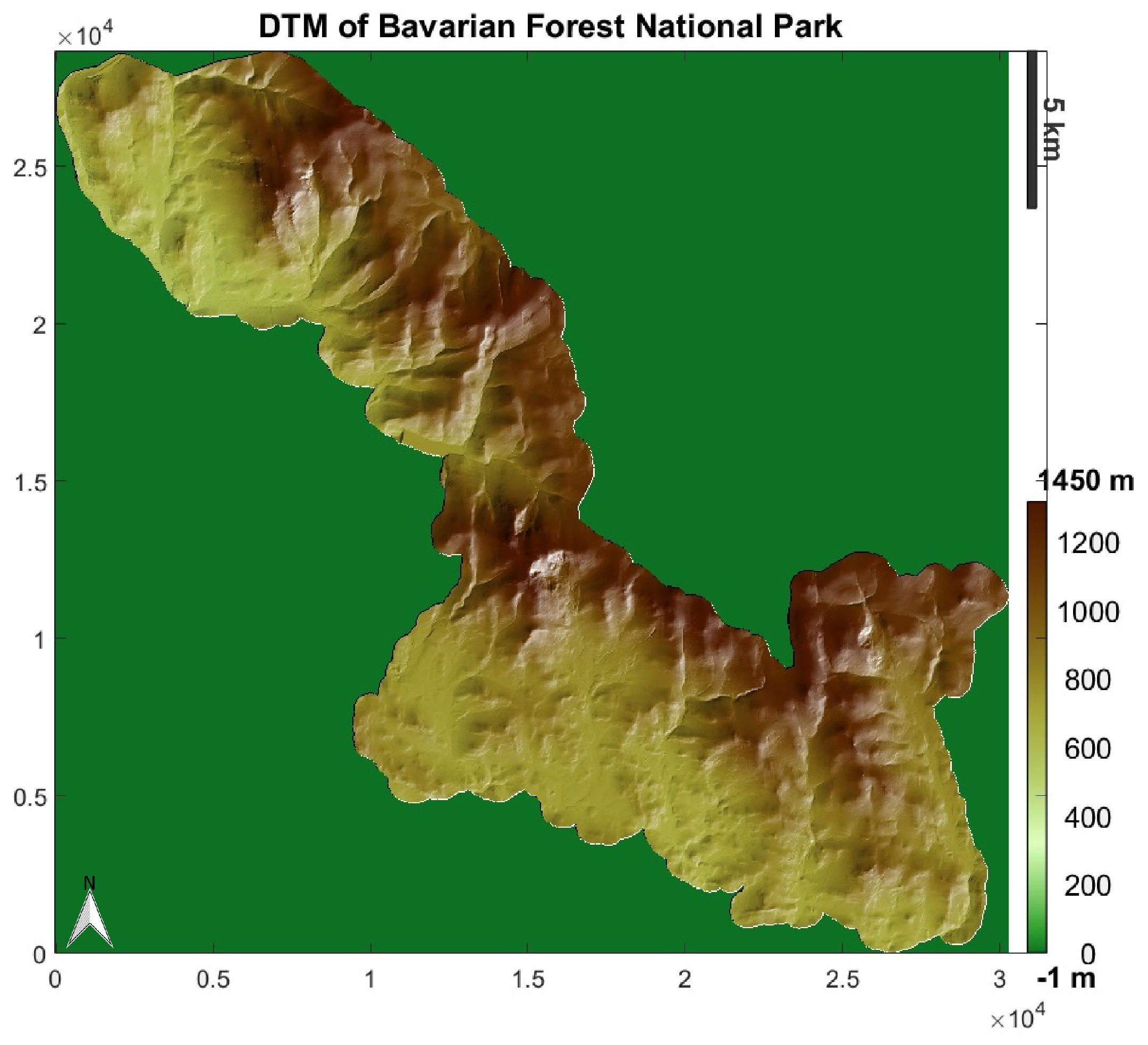
2.1. Study Area
2.2. Height Classification Scheme
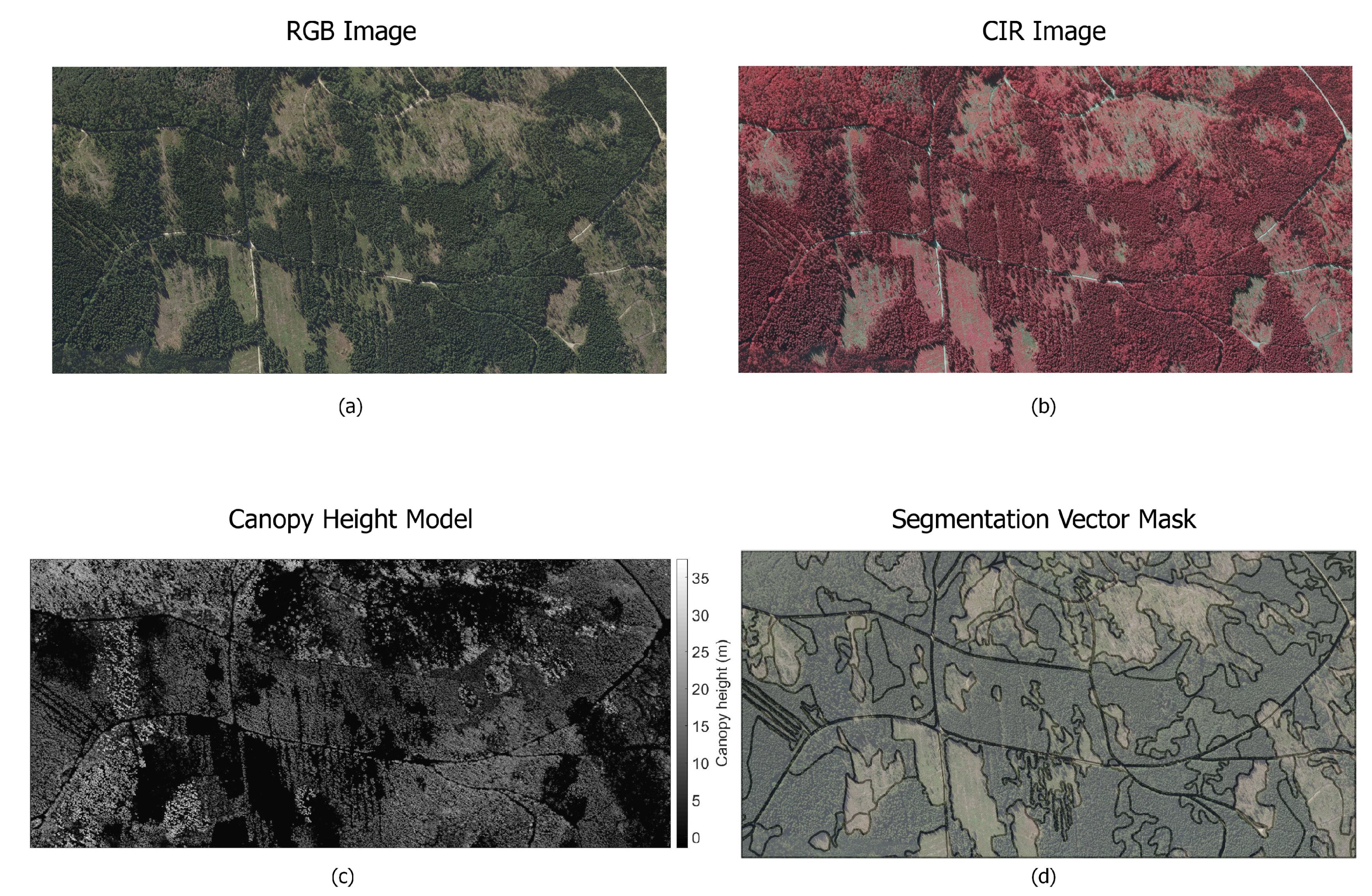
2.3. Dataset
3. Methodology
3.1. Texture Feature Extraction
3.2. Handling of Indefinite Values, Outlier Removal, and Data Normalization
- -
- The first approach, coded as Feat with the derived dataset Feat. dataset, refers to the exclusion of one or more features from the classification process, which have missing data to at least one object. By reducing the number of final features used for each object, memory requirements and classification processing cost are reduced; however, the resulting feature vector may have significantly less discriminatory power compared to the entire set;
- -
- In the second approach, known as listwise deletion, case deletion, or complete-case analysis, objects with missing data to at least one texture feature are excluded, reducing the number of finally classified objects and affecting the representativeness of the results. Listwise deletion, coded as Obj with the derived dataset Obj. dataset, is supported by the fact that the assumption that missingness is not related to the observed and missing variables, i.e., missing-completely-at-random (MCAR) assumption [53] is not valid for the missing data;
- -
- In the third approach, coded as MI with the derived dataset MI. dataset, a multiple imputation technique of the missing data with approximated values is evaluated and employed. In particular, the Amelia II method [54] is used, based on the assumption that the values are drawn from a multivariate gaussian distribution, instead of drawing values from an unconditional distribution, where the missing data are filled in by randomly selected values among the observed ones. Five (5) complete datasets, including the values of all features from every image band, are created, averaged into one set to be used in the classification process. Five imputations have been selected as a good trade-off between efficiency and processing time, according to the formula proposed by Rubin [55].
3.3. Classification
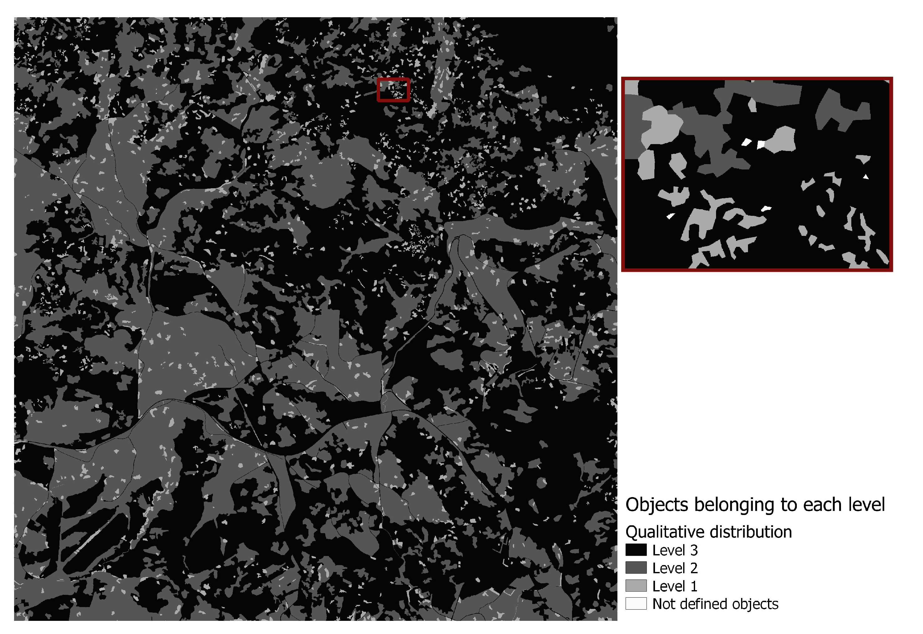
3.4. Multiresolution Analysis
3.5. Validation
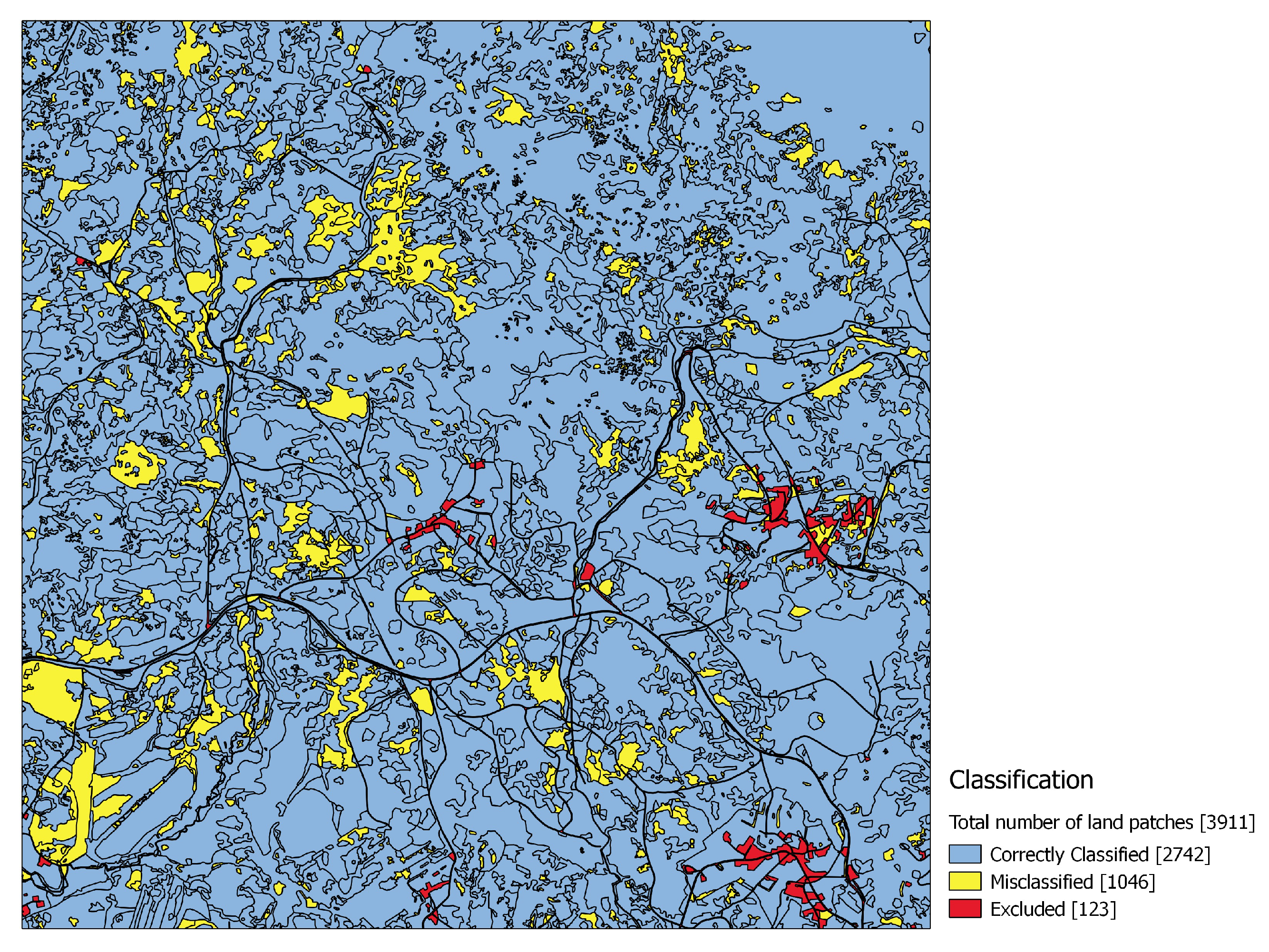
4. Results
4.1. Phase 1: Estimation of Canopy Height Using Ultra-High Resolution Airborne Imagery of 40 cm
4.2. Phase 2: Estimation of Canopy Height Using Spaceborne Spatial Resolution of 10 m
4.3. Phase 3: Fusion of Spatial Resolutions in Hierarchical Mode—Multiresolution Analysis
5. Discussion
6. Conclusions
Author Contributions
Funding
Acknowledgments
Conflicts of Interest
Abbreviations
| A-J48 | AdaBoost.M1 with J48 as basis classifier |
| A-RT | AdaBoost.M1 with REPTree as basis classifier |
| BFNP | Bavarian Forest National Park |
| B-J48 | Bagging with J48 as basis classifier |
| B-RT | Bagging with REPTree as basis classifier |
| CHM | Canopy Height Model |
| DCH | Dwarf chamaephytes (TRS) |
| DEM | Digital Elevation Model |
| DSM | Digital Surface Model |
| DTM | Digital Terrain Model |
| FPH | Forest phanerophytes (TRS) |
| GHC | General Habitat Categories |
| GSD | Ground Sampling Distance |
| J48 | J48 implementation of C4.5 tree classifier |
| LC | Land Cover |
| LV | Local Variance |
| LE | Local Entropy |
| LER | Local Entropy Ratio |
| LPH | Low phanerophytes (TRS) |
| LTBP | Local Binary Patterns with range |
| LTP | Local Ternary Patterns |
| MRA | Multiresolution Analysis |
| MPH | Mid phanerophytes (TRS) |
| OA | Overall Accuracy |
| PA | Producer’s Accuracy |
| RF | Random Forest |
| SCH | Shrubby Chamaephytes (TRS) |
| SVM | Support Vector Machines |
| SVM-M | SVM with fitting logistic models to the output |
| TPH | Tall Phanerophytes (TRS) |
| TRS | Trees and Shrubs |
| UA | User’s Accuracy |
| VHR | Very High Resolution |
Appendix A


References
- Thomas, R.Q.; Hurtt, G.C.; Dubayah, R.; Schilz, M.H. Using lidar data and a height-structured ecosystem model to estimate forest carbon stocks and fluxes over mountainous terrain. Can. J. Remote Sens. 2008, 34, 351–363. [Google Scholar] [CrossRef]
- Goetz, S.; Steinberg, D.; Dubayah, R.; Blair, B. Laser remote sensing of canopy habitat heterogeneity as a predictor of bird species richness in an eastern temperate forest, USA. Remote Sens. Environ. 2007, 108, 254–263. [Google Scholar] [CrossRef]
- Wang, X.; Ouyang, S.; Sun, O.J.; Fang, J. Forest biomass patterns across northeast China are strongly shaped by forest height. For. Ecol. Manag. 2013, 293, 149–160. [Google Scholar] [CrossRef]
- Anderson, J.; Martin, M.; Smith, M.L.; Dubayah, R.; Hofton, M.; Hyde, P.; Peterson, B.; Blair, J.; Knox, R. The use of waveform lidar to measure northern temperate mixed conifer and deciduous forest structure in New Hampshire. Remote Sens. Environ. 2006, 105, 248–261. [Google Scholar] [CrossRef]
- Astola, H.; Häme, T.; Sirro, L.; Molinier, M.; Kilpi, J. Comparison of Sentinel-2 and Landsat 8 imagery for forest variable prediction in boreal region. Remote Sens. Environ. 2019, 223, 257–273. [Google Scholar] [CrossRef]
- Lang, N.; Schindler, K.; Wegner, J.D. Country-Wide High-Resolution Vegetation Height Mapping with Sentinel-2. 2019. Available online: http://xxx.lanl.gov/abs/1904.13270v1 (accessed on 1 December 2019).
- Fang, Z.; Cao, C. Estimation of Forest Canopy Height Over Mountainous Areas Using Satellite Lidar. IEEE J. Sel. Top. Appl. Earth Obs. Remote Sens. 2014, 7, 3157–3166. [Google Scholar] [CrossRef]
- Wang, X.; Huang, H.; Gong, P.; Liu, C.; Li, C.; Li, W. Forest Canopy Height Extraction in Rugged Areas with ICESat / GLAS Data. IEEE Trans. Geosci. Remote Sens. 2014, 52, 4650–4657. [Google Scholar] [CrossRef]
- Hyyppä, J.; Yu, X.; Hyyppä, H.; Vastaranta, M.; Holopainen, M.; Kukko, A.; Kaartinen, H.; Jaakkola, A.; Vaaja, M.; Koskinen, J.; et al. Advances in forest inventory using airborne laser scanning. Remote Sens. 2012, 4, 1190–1207. [Google Scholar] [CrossRef]
- Heurich, M. Automatic recognition and measurement of single trees based on data from airborne laser scanning over the richly structured natural forests of the Bavarian Forest National Park. For. Ecol. Manag. 2008, 255, 2416–2433. [Google Scholar] [CrossRef]
- Hyde, P.; Dubayah, R.; Walker, W.; Blair, J.B.; Hofton, M.; Hunsaker, C. Mapping forest structure for wildlife habitat analysis using multi-sensor (LiDAR, SAR/InSAR, ETM+, Quickbird) synergy. Remote Sens. Environ. 2006, 102, 63–73. [Google Scholar] [CrossRef]
- St-Onge, B.; Hu, Y.; Vega, C. Mapping the height and above-ground biomass of a mixed forest using lidar and stereo Ikonos images. Int. J. Remote Sens. 2008, 29, 1277–1294. [Google Scholar] [CrossRef]
- Lefsky, M.A. A global forest canopy height map from the moderate resolution imaging spectroradiometer and the geoscience laser altimeter system. Geophys. Res. Lett. 2010, 37, 1–5. [Google Scholar] [CrossRef]
- Maltamo, M.; Naesset, E.; Vauhkonen, J. Forestry Applications of Airborne Laser Scanning. Concepts and Case Studies; Managing Forest Ecosystems; Springer: Dordrecht, The Netherlands, 2014; Volume 27, p. 460. [Google Scholar] [CrossRef]
- Kugler, F.; Schulze, D.; Hajnsek, I.; Pretzsch, H.; Papathanassiou, K.P. TanDEM-X Pol-InSAR performance for forest height estimation. IEEE Trans. Geosci. Remote Sens. 2014, 52, 6404–6422. [Google Scholar] [CrossRef]
- Chen, H.; Cloude, S.R.; Goodenough, D.G. Forest Canopy Height Estimation Using Tandem-X Coherence Data. IEEE J. Sel. Top. Appl. Earth Obs. Remote Sens. 2016, 9, 3177–3188. [Google Scholar] [CrossRef]
- Arnaubec, A.; Roueff, A.; Dubois-Fernandez, P.C.; Réfrégier, P. Vegetation Height Estimation Precision With Compact PolInSAR and Homogeneous Random Volume Over Ground Model. IEEE Trans. Geosci. Remote Sens. 2014, 52, 1879–1891. [Google Scholar] [CrossRef]
- Kellndorfer, J.; Cartus, O.; Bishop, J.; Walker, W.; Holecz, F. Large Scale Mapping of Forests and Land Cover with Synthetic Aperture Radar Data. In Land Applications of Radar Remote Sensing; Holecz, F., Pasquali, P., Milisavljevic, N., Closson, D., Eds.; IntechOpen: Rijeka, Croatia, 2014; Chapter 2. [Google Scholar] [CrossRef]
- Vastaranta, M.; Niemi, M.; Karjalainen, M.; Peuhkurinen, J.; Kankare, V.; Hyyppä, J.; Holopainen, M. Prediction of Forest Stand Attributes Using TerraSAR-X Stereo Imagery. Remote Sens. 2014, 6, 3227–3246. [Google Scholar] [CrossRef]
- Perko, R.; Raggam, H.; Gutjahr, K.; Schardt, M. The capabilities of TerraSAR-X imagery for retrieval of forest parameters. Int. Arch. Photogramm. Remote Sens. Spat. Inf. Sci. ISPRS Arch. 2010, 38, 452–456. [Google Scholar]
- St-Onge, B.; Vega, C.; Fournier, R.A.; Hu, Y. Mapping canopy height using a combination of digital stereo-photogrammetry and lidar. Int. J. Remote Sens. 2008, 29, 3343–3364. [Google Scholar] [CrossRef]
- Næsset, E. Determination of Mean Tree Height of Forest Stands by Digital Photogrammetry. Scand. J. For. Res. 2002, 17, 446–459. [Google Scholar] [CrossRef]
- Kellndorfer, J.; Walker, W.; Pierce, L.; Dobson, C.; Fites, J.A.; Hunsaker, C.; Vona, J.; Clutter, M. Vegetation height estimation from Shuttle Radar Topography Mission and National Elevation Datasets. Remote Sens. Environ. 2004, 93, 339–358. [Google Scholar] [CrossRef]
- Baltsavias, E.P. A comparison between photogrammetry and laser scanning. ISPRS J. Photogramm. Remote Sens. 1999, 54, 83–94. [Google Scholar] [CrossRef]
- Miller, D.R.; Quine, C.P.; Hadley, W. An investigation of the potential of digital photogrammetry to provide measurements of forest characteristics and abiotic damage. For. Ecol. Manag. 2000, 135, 279–288. [Google Scholar] [CrossRef]
- Takaku, J.; Tadono, T. PRISM On-Orbit Geometric Calibration and DSM Performance. IEEE Trans. Geosci. Remote Sens. 2009, 47, 4060–4073. [Google Scholar] [CrossRef]
- Stojanova, D.; Panov, P.; Gjorgjioski, V.; Kobler, A.; Džeroski, S. Estimating vegetation height and canopy cover from remotely sensed data with machine learning. Ecol. Inform. 2010, 5, 256–266. [Google Scholar] [CrossRef]
- Dong, L.; Wu, B. A Comparison of Estimating Forest Canopy Height Integrating Multi-Sensor Data Synergy—A Case Study in Mountain Area of Three Gorges. In The International Archives of the Photogrammetry, Remote Sensing and Spatial Information Sciences; ISPRS: Beijing, China, 2008; Volume 37, pp. 379–384. [Google Scholar]
- Jia, Y.; Niu, B.; Zhao, C.; Zhou, L. Estimate the height of vegetation using remote sensing in the groundwater-fluctuating belt in the lower reaches of Heihe River, northwest China. In Proceedings of the 2010 Second IITA International Conference on Geoscience and Remote Sensing, Qingdao, China, 28–31 August 2010; Volume 2, pp. 507–510. [Google Scholar] [CrossRef]
- Anderson, M.C.; Neale, C.M.U.; Li, F.; Norman, J.M.; Kustas, W.P.; Jayanthi, H.; Chavez, J. Upscaling ground observations of vegetation water content, canopy height, and leaf area index during SMEX02 using aircraft and Landsat imagery. Remote Sens. Environ. 2004, 92, 447–464. [Google Scholar] [CrossRef]
- Puhr, C.B.; Donoghue, D.N.M. Remote sensing of upland conifer plantations using Landsat TM data: A case study from Galloway, south-west Scotland. Int. J. Remote Sens. 2010, 21, 633–646. [Google Scholar] [CrossRef]
- Wolter, P.T.; Townsend, P.A.; Sturtevant, B.R. Estimation of forest structural parameters using 5 and 10 meter SPOT-5 satellite data. Remote Sens. Environ. 2009, 113, 2019–2036. [Google Scholar] [CrossRef]
- Petrou, Z.I.; Manakos, I.; Stathaki, T.; Mucher, C.A.; Adamo, M. Discrimination of Vegetation Height Categories With Passive Satellite Sensor Imagery Using Texture Analysis. IEEE J. Sel. Top. Appl. Earth Obs. Remote Sens. 2015, 8, 1442–1455. [Google Scholar] [CrossRef]
- Huang, X.; Zhang, L.; Wang, L. Evaluation of Morphological Texture Features for Mangrove Forest Mapping and Species Discrimination Using Multispectral IKONOS Imagery. IEEE Geosci. Remote Sens. Lett. 2009, 6, 393–397. [Google Scholar] [CrossRef]
- Miyamoto, E.; Merryman, T., Jr. Fast Calculation of Haralick Texture Features; Human Computer Interaction Institute Department of Electrical and Computer Engineering Carnegie Mellon University: Pittsburgh, PA, USA, 2011; Volume 15213, pp. 1–6. [Google Scholar]
- Chowdhury, P.R.; Deshmukh, B.; Goswami, A.K.; Prasad, S.S. Neural network based dunal landform mapping from multispectral images using texture features. J. Sel. Top. Appl. 2011, 4, 171–184. [Google Scholar] [CrossRef]
- Beguet, B.; Chehata, N.; Boukir, S.; Guyon, D. Retrieving forest structure variables from very high resolution satellite images using an automatic method. ISPRS Ann. Photogramm. Remote Sens. Spat. Inf. Sci. 2012, I–7, 1–6. [Google Scholar] [CrossRef]
- Sarkar, A.; Biswas, M.K.; Kartikeyan, B.; Kumar, V.; Majumder, K.L.; Pal, D.K. A MRF model-based segmentation approach to classification for multispectral imagery. IEEE Trans. Geosci. Remote Sens. 2002, 40, 1102–1113. [Google Scholar] [CrossRef]
- Planinsic, P.; Singh, J.; Gleich, D. SAR Image Categorization Using Parametric and Nonparametric Approaches Within a Dual Tree CWT. IEEE Geosci. Remote Sens. 2014, 11, 1757–1761. [Google Scholar] [CrossRef]
- Kayitakire, F.; Hamel, C.; Defourny, P. Retrieving forest structure variables based on image texture analysis and IKONOS-2 imagery. Remote Sens. Environ. 2006, 102, 390–401. [Google Scholar] [CrossRef]
- Aptoula, E. Remote sensing image retrieval with global morphological texture descriptors. IEEE Trans. Geosci. Remote Sens. 2014, 52, 3023–3034. [Google Scholar] [CrossRef]
- Chen, G.; Hay, G.J.; Castilla, G.; St-Onge, B.; Powers, R. A multiscale geographic object-based image analysis to estimate lidar-measured forest canopy height using quickbird imagery. Int. J. Geogr. Inform. Sci. 2011, 25, 877–893. [Google Scholar] [CrossRef]
- Bunce, R.G.H.; Metzger, M.J.; Jongman, R.H.G.; Brandt, J.; De Blust, G.; Elena-Rossello, R.; Groom, G.B.; Halada, L.; Hofer, G.; Howard, D.C.; et al. A standardized procedure for surveillance and monitoring European habitats and provision of spatial data. Landsc. Ecol. 2008, 23, 11–25. [Google Scholar] [CrossRef]
- Cailleret, M.; Heurich, M.; Bugmann, H. Reduction in browsing intensity may not compensate climate change effects on tree species composition in the Bavarian Forest National Park. For. Ecol. Manag. 2014, 328, 179–192. [Google Scholar] [CrossRef]
- Yao, W.; Krzystek, P.; Heurich, M. Tree species classification and estimation of stem volume and DBH based on single tree extraction by exploiting airborne full-waveform LiDAR data. Remote Sens. Environ. 2012, 123, 368–380. [Google Scholar] [CrossRef]
- Latifi, H.; Fassnacht, F.E.; Müller, J.; Tharani, A.; Dech, S.; Heurich, M. Forest inventories by LiDAR data: A comparison of single tree segmentation and metric-based methods for inventories of a heterogeneous temperate forest. Int. J. Appl. Earth Obs. Geoinf. 2015, 42, 162–174. [Google Scholar] [CrossRef]
- Silveyra Gonzalez, R.; Latifi, H.; Weinacker, H.; Dees, M.; Koch, B.; Heurich, M. Integrating LiDAR and high-resolution imagery for object-based mapping of forest habitats in a heterogeneous temperate forest landscape. Int. J. Remote Sens. 2018, 39, 8859–8884. [Google Scholar] [CrossRef]
- Smits, P.C.; Dellepiane, S.G.; Schowengerdt, R.A. Quality assessment of image classification algorithms for land-cover mapping: A review and a proposal for a cost-based approach. Int. J. Remote Sens. 1999, 20, 1461–1486. [Google Scholar] [CrossRef]
- Congalton, R.G. A review of assessing the accuracy of classifications of remotely sensed data. Remote Sens. Environ. 1991, 37, 35–46. [Google Scholar] [CrossRef]
- Kalkhan, M.A.; Reich, R.M.; Czaplewski, R.L. Variance Estimates and Confidence Intervals for the Kappa Measure of Classification Accuracy. Can. J. Remote Sens. 1997, 23, 210–216. [Google Scholar] [CrossRef]
- Petrou, Z.I.; Tarantino, C.; Adamo, M.; Blonda, P.; Petrou, M. Estimation of Vegetation Height Through Satellite Image Texture Analysis. Int. Arch. Photogramm. Remote Sens. Spat. Inf. Sci. 2012, 321–326. [Google Scholar] [CrossRef]
- Petrou, M.; García-Sevilla, P. Image Processing: Dealing with Texture; Wiley: Hoboken, NJ, USA, 2006; Chapter 2; pp. 297–606. [Google Scholar] [CrossRef]
- Little, R.J.A.; Rubin, D.B. Statistical Analysis with Missing Data; John Wiley & Sons, Inc.: New York, NY, USA, 1986. [Google Scholar]
- Honaker, J.; King, G.; Blackwell, M. AMELIA II: A Program for Missing Data. J. Stat. Softw. 2011, 45, 1–54. [Google Scholar] [CrossRef]
- Rubin, D.B. Inference and missing data. Biometrika 1976, 63, 581–592. [Google Scholar] [CrossRef]
- Theodoridis, S.; Koutroumbas, K. Feature Selection. In Pattern Recognition, 4th ed.; Academic Press: Boston, MA, USA, 2009; Chapter 5; pp. 261–322. [Google Scholar] [CrossRef]
- Witten, I.H.; Frank, E.; Hall, M.A. Data Mining: Practical Machine Learning Tools and Techniques, 3rd ed.; Morgan Kaufmann: San Mateo, CA, USA, 2011; p. 664. [Google Scholar] [CrossRef]
- Prasad, A.M.; Iverson, L.R.; Liaw, A. Newer Classification and Regression Tree Techniques: Bagging and Random Forests for Ecological Prediction. Ecosystems 2006, 9, 181–199. [Google Scholar] [CrossRef]
- Gislason, P.O.; Benediktsson, J.A.; Sveinsson, J.R. Random Forests for land cover classification. Pattern Recognit. Lett. 2006, 27, 294–300. [Google Scholar] [CrossRef]
- Leitloff, J.; Hinz, S.; Stilla, U. Vehicle detection in very high resolution satellite images of city areas. IEEE Trans. Geosci. Remote Sens. 2010, 48, 2795–2806. [Google Scholar] [CrossRef]
- Dalponte, M.; Bruzzone, L.; Gianelle, D. Fusion of Hyperspectral and LIDAR Remote Sensing Data for Classification of Complex Forest Areas. IEEE Trans. Geosci. Remote Sens. 2008, 46, 1416–1427. [Google Scholar] [CrossRef]
- Foody, G.M.; Mathur, A. A relative evaluation of multiclass image classification by support vector machines. IEEE Trans. Geosci. Remote Sens. 2004, 42, 1335–1343. [Google Scholar] [CrossRef]
- Quinlan, R. C4.5: Programs for Machine Learning; Morgan Kaufmann Publishers: San Mateo, CA, USA, 1993. [Google Scholar]
- Breiman, L. Random forests. Mach. Learn. 2001, 45, 5–32. [Google Scholar] [CrossRef]
- Breiman, L. Bagging Predictors. Mach. Learn. 1996, 24, 123–140. [Google Scholar] [CrossRef]
- Freund, Y.; Schapire, R.E. Experiments with a new boosting algorithm. In Proceedings of the 13th International Conference on Machine Learning; Morgan Kaufmann Publishers Inc.: San Mateo, CA, USA, 1996; pp. 148–156. [Google Scholar]
- Platt, J. Fast Training of Support Vector Machines Using Sequential Minimal Optimization. In Advances in Kernel Methods—Support Vector Learning; Schölkopf, B., Burges, C.J.C., Smola, A.J., Eds.; MIT Press: Cambridge, MA, USA, 1998; Chapter 12; pp. 185–208. [Google Scholar]
- Hastie, T.; Tibshirani, R. Classification by pairwise coupling. Ann. Stat. 1998, 26, 451–471. [Google Scholar] [CrossRef]
- Roelfsema, C.M.; Lyons, M.; Kovacs, E.M.; Maxwell, P.; Saunders, M.I.; Samper-Villarreal, J.; Phinn, S.R. Multi-temporal mapping of seagrass cover, species and biomass: A semi-automated object based image analysis approach. Remote Sens. Environ. 2014, 150, 172–187. [Google Scholar] [CrossRef]
- Xu, L.; Li, J.; Brenning, A. A comparative study of different classification techniques for marine oil spill identification using RADARSAT-1 imagery. Remote Sens. Environ. 2014, 141, 14–23. [Google Scholar] [CrossRef]
- Franke, J.; Navratil, P.; Keuck, V.; Peterson, K.; Siegert, F. Monitoring Fire and Selective Logging Activities in Tropical Peat Swamp Forests. IEEE J. Sel. Top. Appl. Earth Obs. Remote Sens. 2012, 5, 1811–1820. [Google Scholar] [CrossRef]
- Delalieux, S.; Somers, B.; Haest, B.; Spanhove, T.; Vanden Borre, J.; Mücher, C.A. Heathland conservation status mapping through integration of hyperspectral mixture analysis and decision tree classifiers. Remote Sens. Environ. 2012, 126, 222–231. [Google Scholar] [CrossRef]
- Nelson, M.D.; McRoberts, R.E.; Holden, G.R.; Bauer, M.E. Effects of satellite image spatial aggregation and resolution on estimates of forest land area. Int. J. Remote Sens. 2009, 30, 1913–1940. [Google Scholar] [CrossRef]
- Hansen, M.C.; Potapov, P.V.; Goetz, S.J.; Turubanova, S.; Tyukavina, A.; Krylov, A.; Kommareddy, A.; Egorov, A. Mapping tree height distributions in Sub-Saharan Africa using Landsat 7 and 8 data. Remote Sens. Environ. 2016, 185, 221–232. [Google Scholar] [CrossRef]
- Tyukavina, A.; Baccini, A.; Hansen, M.C.; Potapov, P.V.; Stehman, S.V.; Houghton, R.A.; Krylov, A.M.; Turubanova, S.; Goetz, S.J. Aboveground carbon loss in natural and managed tropical forests from 2000 to 2012. Environ. Res. Lett. 2015, 10. [Google Scholar] [CrossRef]
- Ota, T.; Ahmed, O.S.; Franklin, S.E.; Wulder, M.A.; Kajisa, T.; Mizoue, N.; Yoshida, S.; Takao, G.; Hirata, Y.; Furuya, N.; et al. Estimation of Airborne Lidar-Derived Tropical Forest Canopy Height Using Landsat Time Series in Cambodia. Remote Sens. 2014, 6, 10750–10772. [Google Scholar] [CrossRef]
- Petrou, Z.; Stathaki, T.; Manakos, I.; Adamo, M.; Tarantino, C.; Blonda, P. Land cover to habitat map conversion using remote sensing data: A supervised learning approach. In Proceedings of the IEEE International Geoscience and Remote Sensing Symposium (IGARSS), Quebec City, QC, Canada, 13–18 July 2014; pp. 4683–4686. [Google Scholar] [CrossRef]
- Chrysafis, I.; Mallinis, G.; Siachalou, S.; Patias, P. Assessing the relationships between growing stock volume and sentinel-2 imagery in a mediterranean forest ecosystem. Remote Sens. Lett. 2017, 8, 508–517. [Google Scholar] [CrossRef]
- Korhonen, L.; Hadi; Packalen, P.; Rautiainen, M. Comparison of Sentinel-2 and Landsat 8 in the estimation of boreal forest canopy cover and leaf area index. Remote Sens. Environ. 2017, 195, 259–274. [Google Scholar] [CrossRef]
- Meyer, L.H.; Heurich, M.; Beudert, B.; Premier, J.; Pflugmacher, D. Comparison of Landsat-8 and Sentinel-2 data for estimation of leaf area index in temperate forests. Remote Sens. 2019, 11, 1160. [Google Scholar] [CrossRef]
- Aksoy, S.; Akçay, H.G. Multi-resolution segmentation and shape analysis for remote sensing image classification. In Proceedings of the 2nd International Conference on Recent Advances in Space Technologies, Istanbul, Turkey, 9–11 June 2005; pp. 599–604. [Google Scholar] [CrossRef]
- Grigorescu, S.E.; Petkov, N.; Kruizinga, P. Comparison of Texture Features Based on Gabor Filters. IEEE Trans. Image Process. 2002, 11, 1160–1167. [Google Scholar] [CrossRef]
- Van De Wouwer, G.; Scheunders, P.; Van Dyck, D. Statistical texture characterization from discrete wavelet representations. IEEE Trans. Image Process. 1999, 8, 592–598. [Google Scholar] [CrossRef]
- Franklin, J.; Logan, T.L.; Woodcock, C.E.; Strahler, A.H. Coniferous Forest Classification and Inventory Using Landsat and Digital Terrain Data. IEEE Trans. Geosci. Remote Sens. 1986, GE-24, 139–149. [Google Scholar] [CrossRef]


| Class Name | Description | Range (m) | Class Label |
|---|---|---|---|
| Dwarf chamaephytes (DCH) | Dwarf shrubs | [0, 0.05) | 1 |
| Shrubby chamaephytes (SCH) | Under shrubs | [0.05, 0.3) | 2 |
| Low phanerophytes (LPH) | Low shrubs buds | [0.3, 0.6) | 3 |
| Mid phanerophytes (MPH) | Mid shrubs buds | [0.6, 2) | 4 |
| Tall phanerophytes (TPH) | Tall shrubs buds | [2, 5) | 5 |
| Forest phanerophytes (FPH) | Trees | [5, 40) | 6 |
| Texture Feature | Window (pixels) | Parameters |
|---|---|---|
| Local Variance | ||
| LV1 | ||
| LV2 | ||
| Local Entropy | ||
| LE1 | No prior image band scaling | |
| LE2 | Window discretized in 8 values | |
| LE3 | Object discretized in 8 values | |
| LE4 | No prior image band scaling | |
| LE5 | Window discretized in 8 values | |
| LE6 | Object discretized in 8 values | |
| Local Entropy Ratio | ||
| LER1 | () | Inner pixels included |
| LER2 | () | Inner pixels included |
| LER3 | () | Inner pixels excluded |
| LER4 | () | Inner pixels excluded |
| Local Binary Patterns | ||
| LBP1 | Radius 1 | Rotation invariant |
| LBP2 | Radius 1 | Rotation variant |
| LBP3 | Radius 2 | Rotation invariant |
| LBP4 | Radius 2 | Rotation variant |
| Local Ternary Patterns | ||
| LTP1 | Radius 1 | Rotation invariant |
| LTP2 | Radius 1 | Rotation variant |
| LTP3 | Radius 2 | Rotation invariant |
| LTP4 | Radius 2 | Rotation variant |
| Local Binary Patterns variation | ||
| LTBP1 | Radius 1 | Rotation invariant |
| LTBP2 | Radius 1 | Rotation variant |
| LTBP3 | Radius 2 | Rotation invariant |
| LTBP4 | Radius 2 | Rotation variant |
| Metric | Definition | Symbols |
|---|---|---|
| Overall accuracy | : Number of correctly classified samples; N: total number of samples; | |
| Producer’s accuracy (for class A) | : Correctly classified samples to class A; | |
| Omission error (for class A) | ||
| User’s accuracy (for class A) | : total observed samples of class A; : total samples classified to class A; | |
| Commission error (for class A) | ||
| Cohen’s kappa coefficient | : proportion of agreement between classified and observed samples ; : proportion of expected agreement by chance, , C: number of classes, as defined above |
| Experimental Phase | Best Dataset or Dataset Used | Best Classifier | Object-Based Accuracy (%) | Kappa Coefficient | Area-Based Accuracy (%) | Number of Height Classes |
|---|---|---|---|---|---|---|
| Phase 1 | Obj-Norm | SVM.Lin-M | 64.35 | 0.507 | 83.48 | 6 |
| Phase 1 | MI-Norm | B-J48 | 67.77 | 0.550 | 88.99 | 4 |
| Phase 1’ | MI-OR-Norm | SVM.Lin | 64.58 | 0.490 | 82.49 | 6 |
| Phase 1’ | MI-OR-Norm | SVM.Lin | 69.67 | 0.560 | 83.67 | 4 |
| Phase 2 | Obj | A-J48 | 91.11 | 0.811 | 96.31 | 4 |
| Phase 2’ | Obj | SVM.Lin-M | 85.29 | 0.738 | 91.94 | 4 |
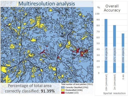
| Phase 3 | Obj | Level 3: A-J48 Level 2: SVM.Lin-M Level 1: SVM.Lin | Level 3: 91.11 Level 2: 80.73 Level 1: 66.55 | Level 3: 0.811 Level 2: 0.684 Level 1: 0.467 | 91.39 | 4 |
| Dataset: Obj-Norm | Predicted Class | ||||||||
|---|---|---|---|---|---|---|---|---|---|
| Classifier: SVM.Lin-M | [0, 0.05) | [0.05, 0.3) | [0.3, 0.6) | [0.6, 2) | [2, 5) | [5, 40) | Sum | PA(%) | |
| Actual Class | [0, 0.05) | 27 | 0 | 2 | 5 | 1 | 0 | 35 | 77.14 |
| [0.05, 0.3) | 4 | 5 | 4 | 12 | 1 | 1 | 27 | 18.51 | |
| [0.3, 0.6) | 1 | 4 | 13 | 21 | 2 | 1 | 42 | 30.95 | |
| [0.6, 2) | 2 | 1 | 4 | 80 | 25 | 8 | 120 | 66.66 | |
| [2, 5) | 1 | 0 | 3 | 27 | 37 | 47 | 115 | 32.17 | |
| [5, 40) | 0 | 0 | 0 | 3 | 20 | 199 | 222 | 89.63 | |
| Sum | 35 | 10 | 26 | 148 | 86 | 256 | 561 | ||
| UA(%) | 77.14 | 0.5 | 0.5 | 54.05 | 43.02 | 77.73 | |||
| Overall accuracy (%): 64.35 | Kappa coefficient: 0.507 | ||||||||
| Dataset: MI-Norm | Predicted Class | ||||||
|---|---|---|---|---|---|---|---|
| Classifier: B-J48 | [0, 0.6) | [0.6, 2) | [2, 5) | [5, 40) | Sum | PA(%) | |
| Actual Class | [0, 0.6) | 103 | 21 | 6 | 5 | 135 | 76.29 |
| [0.6, 2) | 21 | 66 | 22 | 13 | 122 | 54.09 | |
| [2, 5) | 11 | 24 | 40 | 45 | 120 | 33.33 | |
| [5, 40) | 5 | 2 | 20 | 201 | 228 | 88.15 | |
| Sum | 140 | 113 | 88 | 264 | 605 | ||
| UA(%) | 73.57 | 58.40 | 45.45 | 76.13 | |||
| Overall accuracy (%): 67.77 | Kappa coefficient: 0.550 | ||||||
| Dataset: Obj | Predicted Class | ||||||
|---|---|---|---|---|---|---|---|
| Classifier: SVM.Lin-M | [0, 0.6) | [0.6, 2) | [2, 5) | [5, 40) | Sum | PA(%) | |
| Actual Class | [0, 0.6) | 35 | 9 | 0 | 0 | 44 | 79.55 |
| [0.6, 2) | 10 | 78 | 21 | 2 | 111 | 70.27 | |
| [2, 5) | 0 | 18 | 77 | 29 | 124 | 62.09 | |
| [5, 40) | 0 | 1 | 15 | 419 | 435 | 96.32 | |
| Sum | 45 | 106 | 113 | 450 | 714 | ||
| UA(%) | 77.78 | 73.58 | 68.14 | 93.11 | |||
| Overall accuracy (%): 85.29 | Kappa coefficient: 0.738 | ||||||
| Multiresolution Levels | Number of Class Objects | Overall Accuracy (%) | Kappa Coefficient |
|---|---|---|---|
| Level 3–10 m analysis | 90 | 91.11 | 0.812 |
| Level 2–2 m analysis | 1671 | 80.73 | 0.684 |
| Level 1–40 cm analysis | 2006 | 66.55 | 0.47 |
| Not defined | 90 | - | - |
| Total number of objects: 3857 | Percentage of total area classified correctly (%): 91.39 | ||
© 2019 by the authors. Licensee MDPI, Basel, Switzerland. This article is an open access article distributed under the terms and conditions of the Creative Commons Attribution (CC BY) license (http://creativecommons.org/licenses/by/4.0/).
Share and Cite
Boutsoukis, C.; Manakos, I.; Heurich, M.; Delopoulos, A. Canopy Height Estimation from Single Multispectral 2D Airborne Imagery Using Texture Analysis and Machine Learning in Structurally Rich Temperate Forests. Remote Sens. 2019, 11, 2853. https://doi.org/10.3390/rs11232853
Boutsoukis C, Manakos I, Heurich M, Delopoulos A. Canopy Height Estimation from Single Multispectral 2D Airborne Imagery Using Texture Analysis and Machine Learning in Structurally Rich Temperate Forests. Remote Sensing. 2019; 11(23):2853. https://doi.org/10.3390/rs11232853
Chicago/Turabian StyleBoutsoukis, Christos, Ioannis Manakos, Marco Heurich, and Anastasios Delopoulos. 2019. "Canopy Height Estimation from Single Multispectral 2D Airborne Imagery Using Texture Analysis and Machine Learning in Structurally Rich Temperate Forests" Remote Sensing 11, no. 23: 2853. https://doi.org/10.3390/rs11232853
APA StyleBoutsoukis, C., Manakos, I., Heurich, M., & Delopoulos, A. (2019). Canopy Height Estimation from Single Multispectral 2D Airborne Imagery Using Texture Analysis and Machine Learning in Structurally Rich Temperate Forests. Remote Sensing, 11(23), 2853. https://doi.org/10.3390/rs11232853