Circumpolar Thin Arctic Sea Ice Thickness and Small-Scale Roughness Retrieval Using Soil Moisture and Ocean Salinity and Soil Moisture Active Passive Observations

Abstract

The variations in the Arctic sea ice thickness (SIT) due to climate change have both positive and negative effects on commercial human activities, the ecosystem, and the Earth’s environment. Satellite microwave remote sensing based on microwave reflection signals reflected by the sea ice surface has been playing an essential role in monitoring and analyzing the Arctic SIT and sea ice concentration (SIC) during the past decades. Recently, passive microwave satellites incorporating an L-band radiometer, such as soil moisture and ocean salinity (SMOS) and soil moisture active passive (SMAP), have been used for analyzing sea ice characteristics, in addition to land and ocean research. In this study, we present a novel method to estimate thin SIT and sea ice roughness (SIR) using a conversion relationship between them, from the SMAP and SMOS data. Methodologically, the SMAP SIR is retrieved. The SMAP thin SIT and SMOS SIR are estimated using a conversion relationship between thin SIT data from SMOS data and SMAP-derived SIR, which is obtained from the spatial and temporal collocation of the SMOS thin SIT and the SIR retrieved from SMAP. Our results for the Arctic sea ice during December for four consecutive years from 2015 to 2018, show high accuracy (bias = −2.268 cm, root mean square error (RMSE) = 15.919 cm, and correlation coefficient (CC) = 0.414) between the SMOS-provided thin SIT and SMAP-derived SIT, and good agreement (bias = 0.03 cm, RMSE = 0.228 cm, and CC = 0.496) between the SMOS-estimated SIR and SMAP-retrieved SIR. Consequently, our study could be effectively used for monitoring and analyzing the variation in the Arctic sea ice.

1. Introduction

Sea ice is an essential climate variable that is very sensitive to climate change. Sea ice thickness (SIT) ($D_{ice}$) and sea ice concentration (SIC) are important sea ice parameters because of their high sensitivity to heat flux and radiative balance. Recently, in the Arctic region, sea ice extent has been decreasing and SIT has reduced in the past few decades [1,2,3,4,5,6], affecting climate [7,8], Earth’s surface energy budget [9], atmospheric CO2 [10], atmospheric circulation [11], water budget [12], clouds [13], fresh-water [14], and global temperature [15]. Recently, the interannual changes of Arctic sea ice were found to be closely linked to the Arctic cyclone numbers [16], abnormal summer storm activity [17], atmospheric internal variability (AIV) [18], and changes in polar tropospheric and stratospheric circulation [19]. Notably, sea ice coverage has been increasing in the Antarctic in contrast to the decreasing trend in the Arctic [20].

In particular, the reduction of SIT and decrease in the sea ice extent are providing opportunities for commercial human activities such as Northern Sea Route (NSR) [21] shipping, fishing, tourism, and natural resource explorations [22], which have negative impacts on the ecosystem and Arctic environment [23].

Satellite remote sensing using multi-polarization synthetic aperture radar (SAR), radar altimeters [24,25], laser altimeters [26,27], passive microwave radiometers, and optical and infrared sensors, plays a crucial role in monitoring and analyzing the Arctic sea ice properties, because it is difficult to obtain enough in situ measurements and the sensors are capable of global observation, providing plenty of long-term observation data of sea ice with sufficient spectral, spatial, and temporal coverage.

Sea ice surface information, such as SIC and sea ice extent (SIE), has been successfully monitored for more than three decades by the passive microwave sensors such as electrically scanning microwave radiometer (ESMR), scanning multichannel microwave radiometer (SMMR), special sensor microwave imager (SSM/I), advanced microwave scanning radiometer (AMSR), special sensor microwave imager sounder (SSMIS), soil moisture and ocean salinity (SMOS), and soil moisture active passive (SMAP), using a number of algorithms such as the National Aeronautics and Space Administration (NASA) team [28,29], the Bootstrap [30], and many others. The accuracy of the retrieved SIC was reported to be in the range of 5–10% in winter [31,32,33].

However, SIT is known to be more difficult to retrieve from spaceborne sensors than SIC and SIE. In particular, thin SIT (0 to 0.5 m) information is more important for understanding sea ice-atmosphere-ocean interaction through heat flux [34], and for operational and commercial purposes such as weather prediction, ship routing, fishery, and natural resource explorations. However, various in situ methods have limitations in collecting sufficient SIT data. The SIT estimation using a freeboard method, based on the assumption of isostatic equilibrium [24,27], with reflection data from satellite radar altimeters [25], is disadvantageous owing to the validation issue and large uncertainty for SIT < 1.0 m.

In addition, data from satellites with radar altimeters (ICESat and CryoSat-2) or microwave radiometer (SMOS) have been used for SIT estimation. In particular, the SMOS SIT was retrieved using the brightness temperature intensity [35] and the intensity and polarization difference [36]. The SMOS with its microwave imaging radiometer using aperture synthesis (MIRAS) sensor (L-band (frequency = 1.4 GHz, wavelength = 21 cm) radiometer) has a lower uncertainty in estimating thin SIT about 0.5 m under ideal cold conditions [37,38,39], compared with ICESat and CryoSat-2 observations, due to the L-band’s sensitivity to thin SIT variations and the large penetration depth [40].

Surface reflection information is used as an approach for estimating SIC and SIT in passive and active satellite remote sensing. Sea ice reflection is influenced by many geophysical factors, such as wind-roughened sea [28]. In particular, the surface roughness affects the surface reflection by SIC [41,42,43] and has been a difficult parameter to be estimated by satellite remote sensing. Large-scale roughness has been previously modeled using geometric optics [44]. A small-scale sea ice roughness (SIR) ($\sigma$) retrieval and its time-series using a satellite-based passive microwave radiometer were presented [1,45]. Previous studies have shown that the small-scale SIR ranged roughly between 0.2 and 0.6 cm in the Baltic Sea [46] and 0.27 cm in the Beaufort Sea [47]. In SMOS SIT retrieval, the SIR was parameterized as $\sigma = 0.1·D_{ice}$ using the incoherent model instead of the fixed value of SIR using the coherent model [48].

Thus, this study presents a novel method to retrieve SIR and thin SIT (<0.5 m) using a conversion relationship between two variables. We focus on the marginal regions of Arctic sea ice as a study area because of the existence of thin SIT and abrupt changes in SIR. We used the data from the SMAP and SMOS satellites, which incorporate the L-band radiometers. We retrieved SMAP SIR, identified a conversion relationship between SMAP SIR and SMOS thin SIT, and estimated SMAP thin SIT and SMOS SIR in turn.

2. Data

In this study, we used the polarized brightness temperatures ($T_{\mathrm{B},\mathrm{V}}$ and $T_{B,\mathrm{H}}$) and sea ice surface temperatures ($T_{\mathrm{S}}$) of SMAP Level-3 (L3) data, which have 9 km × 9 km spatial resolution and one-day temporal resolution, for estimating the SMAP SIR. In addition, we used the daily SMOS L3C SIT data, with 12.5 km × 12.5 km spatial resolution. The SMOS SIT data are available for winter, from October to April, in the Arctic region. Thus, we consider the SIR and SIT only for the winter season. The study area covers the Arctic sea ice within a circle of latitude from 70°N to 90°N. The study area of the Arctic sea ice was determined using SMAP surface flag information with 9 km spatial resolution, CryoSat-2 L2 data with 5 km spatial resolution from SAR, and interferometric radar altimeter from the European Space Agency (ESA).

3. Method

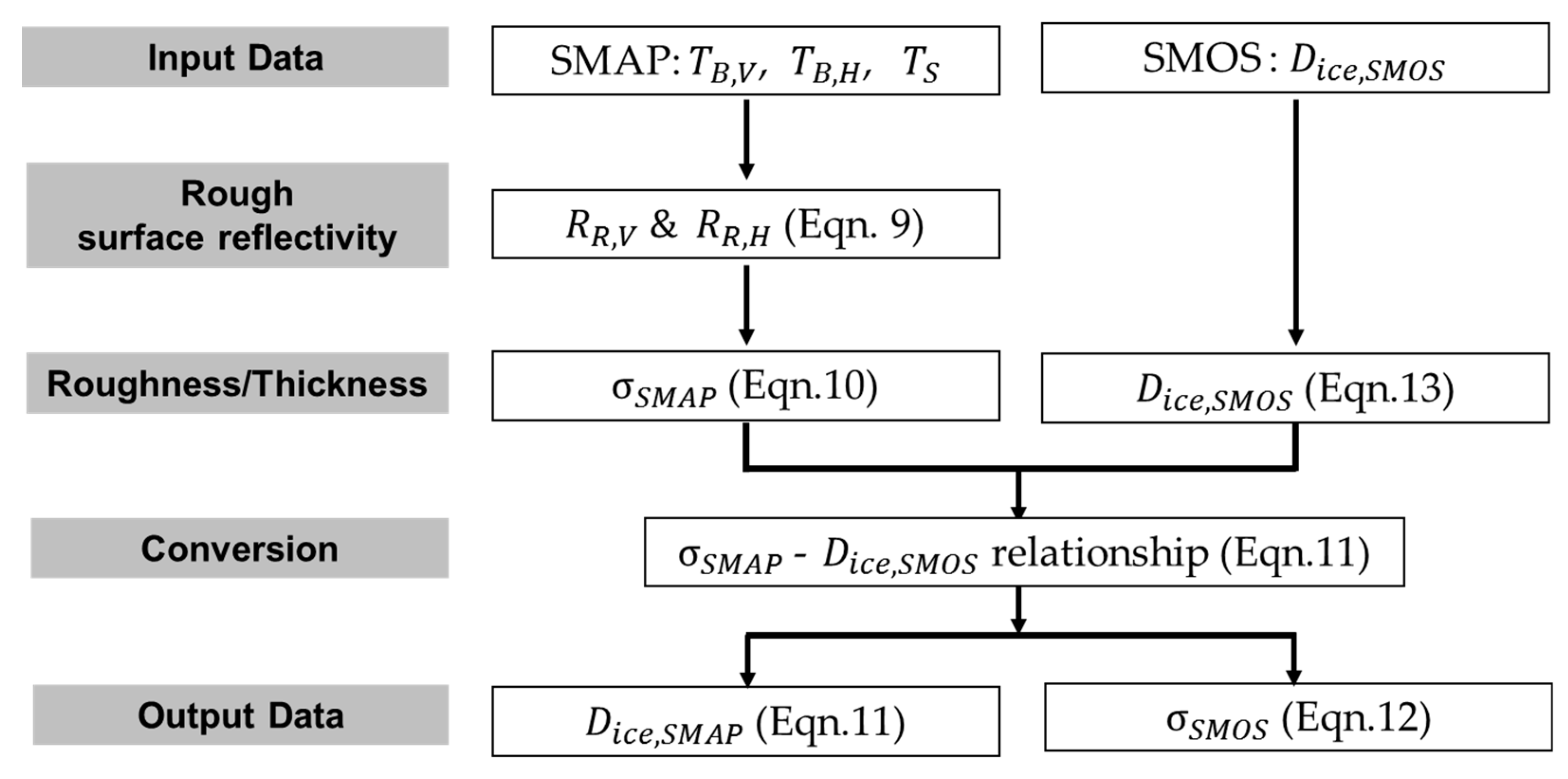
3.1. Retrieval of Soil Moisture Active Passive Sea Ice Roughness (SMAP SIR)

The small-scale SIR affects the surface reflectivity of sea ice. In a semi-empirical model based on the incoherent approach [44], the rough surface reflectivities ($R_{\mathrm{R},\mathrm{P}}$) could be expressed as a function of the specular surface reflectivity ($R_{\mathrm{S},\mathrm{P}}$) and the SIR ($\sigma$), which is a height probability density function with a Gaussian distribution [49,50]. A small-scale SIR retrieval method was developed [8,51] and applied to surface roughness studies on sea ice [1,45].

According to the previous studies, the SIR could be approximately estimated using the following Equations (1) and (2) [8]:

$$\sigma \approx \frac{\lambda }{4\pi \mathit{cos}\theta }\sqrt{\mathit{ln}\left(\frac{{(R_{\mathrm{R},\mathrm{H}})}^{{\mathit{sec}}^2\theta }}{R_{\mathrm{R},\mathrm{V}}}\right)}$$

(1)

$$\sigma \approx \frac{\lambda }{4\pi \mathit{cos}\theta }\sqrt{\mathit{ln}\left(\frac{R_{\mathrm{R},\mathrm{H}}}{R_{\mathrm{R},\mathrm{V}}}\right)+2\mathit{ln}\left(\frac{\sqrt{R_{\mathrm{R},\mathrm{H}}}+\mathit{cos}2\theta }{1+\sqrt{R_{\mathrm{R},\mathrm{H}}}\mathit{cos}2\theta }\right)}$$

(2)

where $\lambda$ is the wavelength (cm), $\theta$ is the viewing angle, $R_{\mathrm{R},\mathrm{V}}$ and $R_{\mathrm{R},\mathrm{H}}$ are the vertically(V)- and horizontally(H)-polarized rough surface reflectivities.

The above two equations were derived by combining the Hong approximation (Equation (3)) [52] and the direct solution (Equation (4)) [53] with the Gaussian distribution (Equation (5)) [49,50] in a semi-empirical model based on the incoherent approach [44] as follows:

$$R_{\mathrm{S},\mathrm{V}} = {(R_{\mathrm{S},\mathrm{H}})}^{{\mathit{sec}}^2\theta }$$

(3)

$$R_{\mathrm{S},\mathrm{H}} = R_{\mathrm{S},\mathrm{V}}\frac{\left(\sqrt{R_{\mathrm{S},\mathrm{V}}}-\mathit{cos}2\theta {)}^2+2\left(\sqrt{R_{\mathrm{S},\mathrm{V}}}-\mathit{Re}({\widehat{r}}_V\right)\mathit{cos}2\theta \right)}{\left(1-\sqrt{R_{\mathrm{S},\mathrm{V}}}\mathit{cos}2\theta {)}^2+2\left(\sqrt{R_{\mathrm{S},\mathrm{V}}}-\mathit{Re}({\widehat{r}}_V\right)\mathit{cos}2\theta \right)}$$

(4)

$$\sigma = \frac{\lambda }{4\pi \mathit{cos}\theta }\sqrt{\mathit{ln}\left(\frac{R_{\mathrm{S},\mathrm{P}}}{R_{\mathrm{R},\mathrm{P}}}\right)}$$

(5)

where $R_{\mathrm{S},\mathrm{V}}$ and $R_{S,\mathrm{H}}$ are the V- and H-polarized specular surface reflectivities. The subscript$\mathrm{P}$ is the V- or H-polarization. $\mathit{Re}({\widehat{r}}_V)$ is the real part of the complex Fresnel reflection coefficient ${\widehat{r}}_V$.

The complex Fresnel reflection coefficient ${\widehat{r}}_V$ is expressed as follows [54]:

$${\widehat{r}}_V = \frac{\mathit{cos}\theta -\sqrt{{\widehat{n}}^2-{\mathit{sin}}^2\theta }}{\mathit{cos}\theta +\sqrt{{\widehat{n}}^2-{\mathit{sin}}^2\theta }}$$

(6)

where $\widehat{n}$ is the complex refractive index.

Equation (5) contains the specular surface reflectivity, which cannot be obtained from satellite observation. Thus, the relationship near the Brewster angle between polarized rough surface reflectivities and specular surface reflectivities was presented as follows [51]:

$$R_{\mathrm{S},\mathrm{V}}>R_{\mathrm{R},\mathrm{V}}$$

(7)

$$R_{\mathrm{S},\mathrm{H}}\approx R_{\mathrm{R},\mathrm{H}}$$

(8)

Therefore, we can obtain Equation (1) after inserting Equation (8) into Equation (5) and replacing $R_{\mathrm{R},\mathrm{V}}$ by the Hong approximation (Equation (3)). Equations (1) and (2) were shown to be effective for melting sea ice and frozen sea ice, respectively [8]. In particular, the surface roughness retrieval method using Equation (1) is useful in microwave satellite remote sensing.

In this study, we focus on thin SIT and SIR. Thus, we used Equation (1) to estimate the SMAP SIR around the edge of the Arctic sea ice. In addition, in this study, sea ice rough surface reflectivity ($R_{\mathrm{R},\mathrm{P}}$) is determined from SMAP satellite data with polarization $P$ = V or H as follows [7]:

$$R_{\mathrm{R},\mathrm{P}} = 1-\frac{T_{\mathrm{B},\mathrm{P}}}{T_{\mathrm{S}}}$$

(9)

Finally, we use the following equation to retrieve the small-scale SIR from the SMAP observation data:

$$\sigma \approx \frac{\lambda }{4\pi \mathit{cos}\theta }·\sqrt{\mathit{ln}\left[\frac{{\left(1-\frac{T_{\mathrm{B},\mathrm{H}}}{T_{\mathrm{S}}}\right)}^{{\mathit{sec}}^2\theta }}{\left(1-\frac{T_{\mathrm{B},\mathrm{V}}}{T_{\mathrm{S}}}\right)}\right]}$$

(10)

where $T_{\mathrm{B},\mathrm{V}}$ and $T_{B,\mathrm{H}}$ are the V- and H-polarized brightness temperatures observed by the SMAP satellite. $T_{\mathrm{S}}$ is the sea ice surface temperature provided by the SMAP satellite at a fixed wavelength $\lambda$ = 21.43 cm at an incidence angle $\theta$ = 40°.

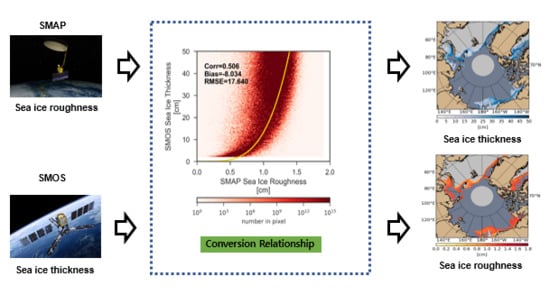
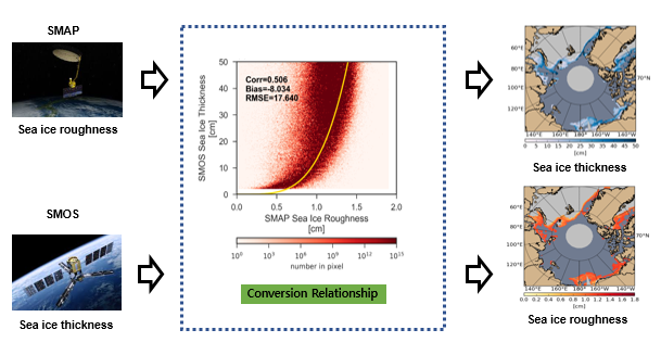
3.2. Conversion Relationship between SIR and SIT

The SMOS satellite provides the SIT ($D_{ice}$) by assuming a homogeneous dielectric-slab of ice thickness [39]. To obtain the conversion relationship between SIT and small-scale SIR, we used the SMOS SIT data and retrieved the SIR using Equation (10) with the data of V- and H-polarized brightness temperatures and sea ice surface temperatures from SMAP. In this study, we used four months of SMOS L3 and SMAP L3 data during Decembers from 2016 to 2018. The conversion relationship between SIT and small-scale SIR is obtained using a regression method as follows:

$$D_{ice, SMOS} = a·{\sigma }_{SMAP}^b$$

(11)

where $D_{ice}$ is the SIT provided by the SMOS data. $\sigma$ is the small-scale SIR estimated using Equation (10) with SMAP-provided brightness temperatures and surface temperature data. $a$ and $b$ are the coefficients to be determined using the collocations of SMAP and SMOS data.

3.3. Retrievals of SMAP SIT and SMOS SIR

In this study, we estimate the SMAP SIT ($D_{ice, SMAP}$) using Equation (11) and SMOS SIR (${\sigma }_{SMOS}$) using the inverse relationship of Equation (11) as follows:

$${\sigma }_{SMOS} = {\left(\frac{D_{ice,SMOS}}{a}\right)}^{\frac{1}{b}}$$

(12)

The SIT from SMOS L3 product is obtained using the iteration method when the difference between the sea ice radiation model (Equation (13)) and thermodynamic models under the condition of a brightness temperature difference of less than 0.1 K, or a SIT difference of less than 1 cm between the two models, as follows [38,39]:

$$D_{ice,SMOS} = -\frac{1}{\gamma }\cdot \ln \left(\frac{T_B-T_1}{T_1-T_0}\right)$$

(13)

where $T_B$ is the brightness temperature from SMOS, $T_0$ is the brightness temperature of open water, $T_1$ is the brightness temperature of infinitely thick sea ice, and $\gamma$ is the attenuation factor. $T_B-T_1$ includes the measurement uncertainty as well as the geophysical uncertainty due to the variability of surface reflectivity. The uncertainty of SMOS L3 SIT was estimated as ±0.02 m/K for $D_{ice,SMOS}$ = 0.4 m [38].

We could obtain another form of SIT as a function of the SMAP or SMOS observations by inserting Equation (10) into Equation (11) as follows:

$$D_{ice} = a·{\left[\frac{\lambda }{4\pi \mathit{cos}\theta }·\sqrt{\mathit{ln}\left[\frac{{\left(1-\frac{T_{\mathrm{B},\mathrm{H}}}{T_{\mathrm{S}}}\right)}^{{\mathit{sec}}^2\theta }}{\left(1-\frac{T_{\mathrm{B},\mathrm{V}}}{T_{\mathrm{S}}}\right)}\right]}\right]}_{}^b$$

(14)

In Equation (14), $T_{\mathrm{B},\mathrm{V}}$, $T_{B,\mathrm{H}}$, and $T_{\mathrm{S}}$ are from the SMAP and SMOS observations. $\lambda$ and $\theta$ are given from the SMAP and SMOS satellites. The unknown variables are $T_1$ and $\gamma$ in the SMOS SIT algorithm (Equation (13)), while they are $a$ and $b$ in our SIT algorithm (Equation (14)). Equation (14) is bias-corrected using the result from December 2017 in this study.

3.4. Validation of SMAP SIT and SMOS SIR

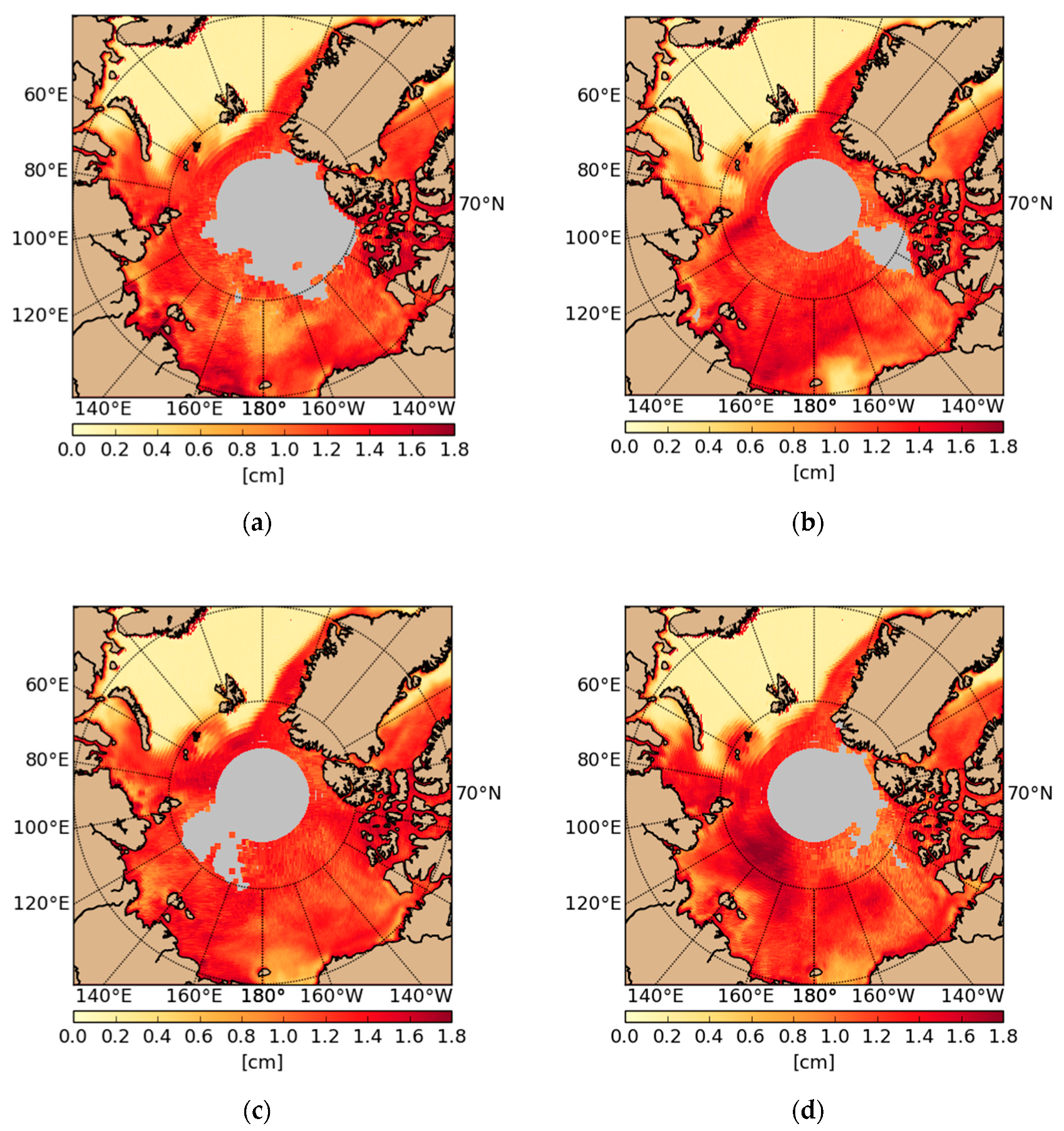
For validation, the pairs of SIRs (${\sigma }_{SMAP}$ and ${\sigma }_{SMOS}$) and SITs ($D_{ice,SMAP}$ and $D_{ice,SMOS}$) are compared for different periods of observation: for December 2015, 2016, and 2018. Figure 1 shows the procedure of this study. As a preprocess, SMAP and SMOS data are collocated temporally and spatially. First, we use V- and H-polarized brightness temperatures and ice surface temperatures from SMAP and SMOS SIT as inputs. We then estimate the V- and H-polarized rough surface reflectivities. The surface roughness retrieval equation is then applied to calculate the V- and H-polarized rough surface reflectivities for computing SIR. Later, we obtain a conversion relationship between SMAP SIR and SMOS SIT, and estimate SMAP SIT and SMOS SIR. Finally, the comparisons between SIRs and SITs from SMAP and SMOS are performed.

4. Results

Figure 2 shows the examples of the SMAP SIR from December of 2015 to 2018 estimated using the proposed method. The retrieved SMAP SIR ranges from approximately 0.01 to 1.81 cm within the thin SMOS SIT. These SIR values include values reported in the previous studies, between 0.2 and 0.6 cm in the Baltic Sea [46], and 0.27 cm in the Beaufort Sea [47]. We can identify that the SIR exhibits a kind of oscillation pattern with positive and negative fluctuations (the SIR shows significant changes). In addition, the average value of SIR tends to decrease as time passes. In this study, we did not investigate the effect of climate change on our SIR because we only have data for four years, which are not sufficient for climate change studies.

Figure 3 shows the scatterplots between the SMAP SIR and SMOS SIT during December of the four consecutive years from 2015 to 2018. The SMAP SIR and SMOS SIT are highly correlated with averaged correlation coefficients (CC) = 0.462 during December for 2015 to 2018. To obtain the best conversion relationship between SMAP SIR and SMOS SIT, we applied a regression method (Equation (14)) to the data for December 2017. Accordingly, we obtained the conversion relationship between SMOS SIT and SMAP SIR with $a$ = 13.27 and $b$ = 4. Figure 3c shows the conversion relationship with the statistical results of CC = 0.506 and root-mean-square-error (RMSE) = 17.640 cm for all the collocated data pixels between SMAP SIR and SMOS SIT during December 2017.

Figure 4 shows the scatterplots between the SMAP-derived SIT and SMOS SIT during December of 2015 to 2018. This result shows the CC = 0.414, bias = −2.268 cm and RMSE = 15.919 cm for all the data pixels between two SITs during December of the years 2015 to 2018. The CC ranges from 0.370 to 0.461. The RMSE, ranging from 15.705 to 16.392, is stable. Figure 4c shows the best statistical results (CC = 0.461, bias = 0.000 cm and RMSE = 15.705 cm) because the conversion relationship between SMOS SIT and SMAP SIR was obtained using the data from December 2017 and was applied to December of 2015, 2016, and 2018.

Figure 5 shows the spatial distributions of the SMOS SIT and SMAP-derived SIT on December 2017. The CC of $D_{ice}$, standard deviation (STD) of the ice thickness $D_{ice}$ from aircraft measurement and of $D_{ice}$ estimated using Equation (13) were 0.5, 0.82 ± 0.4 m, and 0.65 ± 0.3 m for SMOS SIT respectively [38], and 0.88, 0.79 ± 0.5 m, and 0.55 ± 0.4 m for SMOS SIT, respectively [48]. A CC of 0.58 between SMOS–SMAP-derived ice thickness and the ship observations was estimated during the period of October 5 to November 4, 2015, in the Beaufort and Chukchi seas [55]. The values of bias (−0.12 m) and RMSE (0.26 m) from November to December 2018 from the comparison between the Ocean and Sea Ice Satellite Application Facility (OSISAF) and SMOS ice thickness was reported [56]. Therefore, our results show excellent agreement with those estimated by the previous studies.

Figure 6 shows the scatterplots between the SMAP-derived SIR and SMOS-derived SIR during December 2017. This result shows the CC = 0.496, bias = 0.03 cm, and RMSE = 0.228 cm for all the data pixels between two SIRs during the month of December of years 2015 to 2018. Notably, the CC of SIRs is higher than those of SITs between SMAP and SMOS. The CC ranges from 0.441 to 0.542, and the RMSE varies from 0.219 to 0.237 cm. The SIR during December 2017 also shows the best statistical results (CC = 0.542, bias = 0.000 cm and RMSE = 0.219 cm) because of the same conversion relationship between SMAP SIR and SMOS SIT obtained from the data retrieved during December 2017.

Figure 7 shows the spatial distributions of the SMAP SIR (Figure 7a), SMOS-derived SIR (Figure 7b), and the difference map between SMAP SIR and SMOS-derived SIR during December 2017. This result could not be validated because of lack of in situ measurements. The derived SMOS SIR is estimated to be between 0.49 and 1.25 cm, which is lower than the SMAP SIR values from 0.01 to 1.81 cm. The SMOS SIR is higher than SMAP SIR in the Beaufort and Kara Seas, while it is lower than SMAP SIR in the inner part of the circumpolar region. Thus, our SMOS-derived SIR tends to be relatively lower than SMAP SIR as the SIT increases in the circumpolar regions.

5. Summary and Concluding Remarks

The Arctic sea ice is sensitive to climate change and affects Earth’s environment and ecosystems. Nevertheless, the sea ice melting provides an opportunity for commercial human activities. During the past decades, satellite microwave remote sensing has been used for monitoring and analyzing the Arctic SIT and SIC. Physically, the sea ice parameters, such as SIC, SIT, and SIR are estimated from the variation of sea ice surface reflection signals for the different types of sea ice, such as new, young, and multiyear ices. Thus, we assumed the correlation between SIT and SIR derived from L-band radiometer, due to its high sensitivity to SIT variations and large penetration depth.

We retrieved the SIR and presented a novel method to estimate thin SIT and SIR using a conversion relationship between them, using the data of SMAP-retrieved SIR and SMOS-provided thin SIT. Furthermore, this study provided the SMAP thin SIT and SMOS SIR, non-existent data, using the conversion relationship between SMOS thin SIT data and SMAP-derived SIR.

The validation of our results in the Arctic sea ice during winter showed high accuracy (bias = −2.268 cm, RMSE = 15.919 cm, and CC = 0.414) between the SMOS-provided thin SIT and the SMAP-derived SIT, and good agreement (bias = 0.03 cm, RMSE = 0.228 cm, and CC = 0.496) between the SMOS-estimated SIR and the SMAP-retrieved SIR. Consequently, our study contributes with a novel insight into the SIR and SIT retrievals in the Arctic marginal seas during winter, and the Arctic climate change from sea ice variations that are highly correlated with abnormal summer storm activity [17] and cyclone behavior [16,57]. This correlation can be attributed to sea ice variations, especially in their marginal zones, having a high impact on the heat fluxes, atmospheric circulation, and cyclones through strong interaction between the ice-ocean surfaces and atmosphere.

References

1. Hong, S.; Shin, I. Global trends of sea ice: Small-scale roughness and refractive index. J. Clim. 2010, 23, 4669–4676. [Google Scholar] [CrossRef]
2. Johannessen, O.M. Decreasing arctic sea ice mirrors increasing CO2 on decadal time scale. Atmos. Ocean. Sci. Lett. 2008, 1, 51–56. [Google Scholar] [CrossRef]
3. Kwok, R.; Rothrock, D.A. Decline in Arctic sea ice thickness from submarine and ICESat records: 1958–2008. Geophys. Res. Lett. 2009, 36, L15501. [Google Scholar] [CrossRef]
4. Laxon, S.W.; Giles, K.A.; Ridout, A.L.; Wingham, D.J.; Willatt, R.; Cullen, R.; Kwok, R.; Schweiger, A.; Zhang, J.; Haas, C.; et al. CryoSat-2 estimates of Arctic sea ice thickness and volume. Geophys. Res. Lett. 2013, 40, 732–737. [Google Scholar] [CrossRef]
5. Shepherd, A.; Wingham, D.; Wallis, D.; Giles, K.; Laxon, S.W.; Sundal, A.V. Recent loss of floating ice and the consequent sea level contribution. Geophys. Res. Lett. 2010, 37, L13503. [Google Scholar] [CrossRef]
6. Stroeve, J.C.; Kattsov, V.; Barrett, A.; Serreze, M.; Pavlova, T.; Holland, M.; Meier, W.N. Trends in Arctic sea ice extent from CMIP5, CMIP3 and observations. Geophys. Res. Lett. 2012, 39, L16502. [Google Scholar] [CrossRef]
7. Comiso, J.C.; Cavalieri, D.J.; Markus, T. Sea ice concentration, ice temperature, and snow depth using AMSR-E data. IEEE Trans. Geosci. Remote Sens. 2003, 41, 243–252. [Google Scholar] [CrossRef]
8. Hong, S.; Shin, I.; Byun, Y.; Seo, H.-J.; Kim, Y. Analysis of sea ice surface properties using ASH and Hong approximations in satellite remote sensing. Remote Sens. Lett. 2014, 5, 139–147. [Google Scholar] [CrossRef]
9. Gorodetskaya, I.V.; Tremblay, L.B.; Liepert, B.; Cane, M.; Cullather, R.J. The influence of cloud and surface properties on the Arctic Ocean shortwave radiation budget in coupled models. J. Clim. 2008, 21, 866–882. [Google Scholar] [CrossRef]
10. Manabe, S.; Stouffer, R.J. Century-scale effects of increased atmospheric CO2 on the ocean-atmosphere system. Nature 1993, 364, 215–218. [Google Scholar] [CrossRef]
11. Tjernström, M.; Mauritsen, T. Mesoscale variability in the summer Arctic boundary layer. Bound. Layer Meteorol. 2009, 130, 383–406. [Google Scholar] [CrossRef]
12. Gutowski, W.J., Jr. Influence of Arctic wetlands on Arctic atmospheric circulation. J. Clim. 2007, 20, 4243–4254. [Google Scholar] [CrossRef]
13. Abbot, D.S.; Tziperman, E. Controls on the activation and strength of a high-latitude convective cloud feedback. J. Atmos. Sci. 2009, 66, 519–529. [Google Scholar] [CrossRef]
14. Salminen, M.; Pulliainen, J.; Metsämäki, S.; Kontu, A.; Suokanerva, H. The behavior of snow and snow-free surface reflectance in boreal forests: Implications to the performance of snow covered area monitoring. Remote Sens. Environ. 2009, 113, 907–918. [Google Scholar] [CrossRef]
15. Qu, X.; Hall, A. Surface contribution to planetary albedo variability in cryosphere regions. J. Clim. 2005, 18, 5239–5252. [Google Scholar] [CrossRef]
16. Simmonds, I.; Burke, C.; Keay, K. Arctic climate change as manifest in cyclone behavior. J. Clim. 2008, 21, 5777–5796. [Google Scholar] [CrossRef]
17. Screen, J.A.; Simmonds, I.; Keay, K. Dramatic interannual changes of perennial Arctic sea ice linked to abnormal summer storm activity. J. Geophys. Res. 2011, 116, D15105. [Google Scholar] [CrossRef]
18. Screen, J.A.; Deser, C.; Simmonds, I.; Tomas, R. Atmospheric impacts of Arctic sea-ice loss, 1979–2009: Separating forced change from atmospheric internal variability. Clim. Dyn. 2014, 43, 333–344. [Google Scholar] [CrossRef]
19. Screen, J.A.; Bracegirdle, T.J.; Simmonds, I. Polar climate change as manifest in atmospheric circulation. Curr. Clim. Chang. Rep. 2018, 4, 383–395. [Google Scholar] [CrossRef]
20. Parkinson, C.L.; DiGirolamo, N.E. 2016: New visualizations highlight new information on the contrasting Arctic and Antarctic sea-ice trends since the late 1970s. Remote Sens. Environ. 2016, 183, 198–204. [Google Scholar] [CrossRef]
21. Isakov, N.A.; Yakovlev, A.N.; Nikulin, A.E.; Serebryansky, G.Y.; Patrakova, T.A. The NSR Simulation Study Package 3: Potential Cargo Flow Analysis and Economic Evaluation for the Simulation Study (Russian Part); International Northern Sea Route Programme (INSROP Working Paper 139): Lysaker, Norway, 1999; p. 54. [Google Scholar]
22. Meier, W.N.; Hovelsrud, G.K.; van Oort, B.E.H.; Key, J.R.; Kovacs, K.M.; Michel, C.; Haas, C.; Granskog, M.A.; Gerland, S.; Perovich, D.K.; et al. Arctic sea ice in transformation: A review of recent observed changes and impacts on biology and human activity. Rev. Geophys. 2014, 51, 185–217. [Google Scholar] [CrossRef]
23. Johannessen, O.M.; Alexandrov, V.; Sandven, S.; Pettersson, L.H.; Bobylev, L.; Kloster, L. Remote sensing of sea ice in the Northern Sea Route—Studies and applications; Springer Praxis Books: New York, NY, USA, 2007. [Google Scholar]
24. Giles, K.A.; Laxon, S.W.; Ridout, A.L. Circumpolar thinning of Arctic sea ice following the 2007 record ice extent minimum. Geophys. Res. Lett. 2008, 35, L22502. [Google Scholar] [CrossRef]
25. Laxon, S.; Peacock, N.; Smith, D. High interannual variability of sea ice thickness in the Arctic region. Nature 2003, 425, 947–950. [Google Scholar] [CrossRef] [PubMed]
26. Forsberg, R.; Skourup, H. Arctic Ocean gravity, geoid and sea ice freeboard heights from ICESat and GRACE. Geophys. Res. Lett. 2005, 32, L21502. [Google Scholar] [CrossRef]
27. Kwok, R.; Cunningham, G.F.; Wensnahan, M.; Rigor, I.; Zwally, H.J.; Yi, D. Thinning and volume loss of the Arctic Ocean sea ice cover: 2003–2008. J. Geophys. Res. 2009, 114, C07005. [Google Scholar] [CrossRef]
28. Cavalieri, D.J.; Gloersen, P.; Campbell, W.J. Determination of sea ice parameters with the NIMBUS 7 SMMR. J. Geophys. Res. 1984, 89, 5355–5369. [Google Scholar] [CrossRef]
29. Markus, T.; Cavalieri, D.J. An enhanced NASA team sea ice algorithm. IEEE Trans. Geosci. Remote Sens. 2000, 38, 1387–1398. [Google Scholar] [CrossRef]
30. Comiso, J.C. Characteristics of Arctic winter sea ice from satellite multispectral microwave observations. J. Geophys. Res. 1986, 91, 975–994. [Google Scholar] [CrossRef]
31. Belchansky, G.I.; Douglas, D.C. Seasonal comparisons of sea ice concentration estimates derived from SSM/I, OKEAN, and RADARSAT data. Remote Sens. Environ. 2002, 81, 67–81. [Google Scholar] [CrossRef]
32. Emery, W.J.; Fowler, C.; Maslanik, J. Arctic sea ice concentration from special sensor microwave imager and advanced very high resolution radiometer satellite data. J. Geophys. Res. 1994, 99, 18329–18342. [Google Scholar] [CrossRef]
33. Steffen, K.; Schweiger, A. NASA team algorithm for sea ice concentration retrieval from Defense Meteorological Satellite Program Special Sensor Microwave Imager: Comparison with Landsat satellite imagery. J. Geophys. Res. 1991, 96, 21971–21987. [Google Scholar] [CrossRef]
34. Maykut, G.A. Energy exchange over young sea-ice in the central Arctic. J. Geophys. Res. 1978, 83, 3646–3658. [Google Scholar] [CrossRef]
35. Tian-Kunze, X.; Kaleschke, L.; Maaß, N.; Mäkynen, M.; Serra, N.; Drusch, M.; Krumpen, T. SMOS-derived thin sea ice thickness: Algorithm baseline, product specifications and initial verification. Cryosphere 2014, 8, 997–1018. [Google Scholar] [CrossRef] [Green Version]
36. Huntemann, M.; Heygster, G.; Kaleschke, L.; Krumpen, T.; Mäkynen, M.; Drusch, M. Empirical sea ice thickness retrieval during the freeze-up period from SMOS high incident angle observations. Cryosphere 2014, 8, 439–451. [Google Scholar] [CrossRef] [Green Version]
37. Heygster, G.; Hendricks, S.; Kaleschke, L.; Maaß, N.; Mills, P.; Stammer, D.; Tonboe, R.T.; Haas, C. L-Band Radiometry for Sea-Ice Applications; Final Report for ESA ESTEC Contract 21130/08/NL/EL; Institute of Environmental Physics, University of Bremen: Bremen, Germany, 2009. [Google Scholar]
38. Kaleschke, L.; Maaß, N.; Haas, C.; Hendricks, S.; Heygster, G.; Tonboe, R.T. A sea-ice thickness retrieval model for 1.4 GHz radiometry and application to airborne measurements over low salinity sea-ice. Cryosphere 2010, 4, 583–592. [Google Scholar] [CrossRef] [Green Version]
39. Kaleschke, L.; Tian-Kunze, X.; Maaß, N.; Mäkynen, M.; Drusch, M. Sea ice thickness retrieval from SMOS brightness temperatures during the Arctic freeze-up period. Geophys. Res. Lett. 2012, 39, L05501. [Google Scholar] [CrossRef]
40. Mätzler, C. Applications of SMOS over terrestrial ice and snow. In Proceedings of the 3rd SMOS Workshop, DLR, Oberpfaffenhofen, Germany, 10–12 December 2001. [Google Scholar]
41. Petty, G.W. Physical retrievals of over-ocean rain rate from multichannel microwave imagery. Part I: Theoretical characteristics of normalized polarization and scattering indices. Meteorol. Atmos. Phys. 1994, 54, 79–99. [Google Scholar] [CrossRef]
42. Stroeve, J.C.; Markus, T.; Maslanik, J.A.; Cavalieri, D.J.; Gasiewski, A.J.; Heinrichs, J.F.; Holmgren, J.; Perovich, D.K.; Sturm, M. Impact of surface roughness on AMSR-E sea ice products. IEEE Trans. Geosci. Remote Sens. 2006, 44, 3103–3117. [Google Scholar] [CrossRef]
43. Wegmüller, U.; Mätzler, C. Rough bare soil reflectivity model. IEEE Trans. Geosci. Remote Sens. 1999, 37, 1391–1395. [Google Scholar] [CrossRef]
44. Ulaby, F.T.; Moore, R.K.; Fung, A.E. Microwave Remote Sensing: Active and Passive Vol. II: Radar Remote Sensing and Surface Scattering and Emission Theory; Addison-Wesley: Reading, MA, USA, 1982. [Google Scholar]
45. Hong, S. Detection of small-scale roughness and refractive index of sea ice in passive satellite microwave remote sensing. Remote Sens. Environ. 2010, 114, 1136–1140. [Google Scholar] [CrossRef]
46. Manninen, A.T. Surface roughness of Baltic sea ice. J. Geophys. Res. 1997, 102, 1119–1139. [Google Scholar] [CrossRef]
47. Carlstrom, A. Laser profiler for verification of surface scattering models. In Proceedings of the 11th IEEE Geoscience and Remote Sensing Symposium, Espoo, Finland, 3–6 June 1991. [Google Scholar]
48. Kaleschke, L.; Tian-Kunze, X.; Maaß, N.; Beitsch, A.; Wernecke, A.; Miernecki, M.; Müller, G.; Fock, B.H.; Gierisch, A.M.; Schlünzen, K.H.; et al. SMOS sea ice product: Operational application and validation in the Barents Sea marginal ice zone. Remote Sens. Environ. 2016, 180, 264–273. [Google Scholar] [CrossRef]
49. Choudhury, B.; Schumugge, J.; Chang, A.; Newton, R. Effect of surface roughness on the microwave emission from soils. J. Geophys. Res. 1979, 84, 5699–5706. [Google Scholar] [CrossRef]
50. Wu, S.T.; Fung, A.E. A non coherent model for microwave emissions and backscattering from sea surface. J. Geophys. Res. 1972, 77, 5917–5929. [Google Scholar] [CrossRef] [Green Version]
51. Hong, S. Surface roughness and polarization ratio in microwave remote sensing. Int. J. Remote Sens. 2010, 31, 2709–2716. [Google Scholar] [CrossRef]
52. Hong, S. Retrieval of refractive index over specular surfaces for remote sensing applications. J. Appl. Remote Sens. 2009, 3, 033560. [Google Scholar] [CrossRef]
53. Hong, S. Polarization conversion for specular components of surface reflection. IEEE Geosci. Remote Sens. Lett. 2013, 10, 1469–1472. [Google Scholar] [CrossRef]
54. Hechts, E. Optics, 3rd ed.; Addison Wesley Longman: New York, NY, USA, 1998. [Google Scholar]
55. Paţilea, C.; Heygster, G.; Huntemann, M.; Spreen, G. Combined SMAP–SMOS thin sea ice thickness retrieval. Cryosphere 2019, 13, 675–691. [Google Scholar] [CrossRef] [Green Version]
56. Williams, T.; Korosov, A.; Rampal, P.; Ólason, E. Presentation and evaluation of the Arctic sea ice forecasting system neXtSIM-F. Cryosphere 2019. [Google Scholar] [CrossRef] [Green Version]
57. Simmonds, I. Comparing and contrasting the behaviour of Arctic and Antarctic sea ice over the 35-year period 1979–2013. Ann. Glaciol. 2015, 56, 18–28. [Google Scholar] [CrossRef] [Green Version]
Figure 1. A flowchart of the proposed research.
Remotesensing 11 02835 g001
Figure 2. Spatial distributions of soil moisture active passive sea ice roughness (SMAP SIR) during December of (a) 2015, (b) 2016, (c) 2017, and (d) 2018.
Remotesensing 11 02835 g002
Figure 3. Scatter plots between the SMAP SIR and soil moisture and ocean salinity sea ice thickness (SMOS SIT) during the month of December of years: (a) 2015, (b) 2016, (c) 2017, and (d) 2018. In this case, a   =   13.27 and b   =   4 in Equation (14) were applied.
Remotesensing 11 02835 g003
Figure 4. Scatterplots between the SMOS SIT and SMAP-derived SIT during the month of December of years: (a) 2015, (b) 2016, (c) 2017, and (d) 2018.
Remotesensing 11 02835 g004
Figure 5. Spatial distributions of (a) SMOS SIT, (b) SMAP-derived SIT, and (c) SMOS SIT–SMAP-derived SIT during December 2017.
Remotesensing 11 02835 g005
Figure 6. Scatter plots between the SMAP SIR and SMOS-derived SIR during the month of December of years: (a) 2015, (b) 2016, (c) 2017, and (d) 2018.
Remotesensing 11 02835 g006
Figure 7. Spatial distributions of (a) SMAP SIR, (b) SMOS-derived SIR, and (c) SMAP SIR–SMOS-derived SIR during December 2017.
Remotesensing 11 02835 g007