Infrared Small-Faint Target Detection Using Non-i.i.d. Mixture of Gaussians and Flux Density


Abstract
:
1. Introduction
2. The Proposed Model
2.1. Spatio-Temporal Patch Model
2.2. Background Component
2.3. Noise Component
2.4. Variational Inference
2.4.1. Estimation of Noise Component
2.4.2. Estimation of Background Component
2.5. Target Extraction
2.5.1. Selecting Noise Component Containing Target
2.5.2. Extracting Target by MFD
| Algorithm 1 |
| Input: Infrared image sequence . |
| Initialize: Set parameters in noise prior. Low-rank background component and parameters in the model prior , scale parameter in MFD method, iteration number . |
| Step 1: Construct the spatio-temporal patch image with the input infrared image sequence using the method in Section 2.1. |
| Step 2: Build NMoG noise model under the Bayesian framework by Equations (2) and (5). |
| Step 3: While not converged do: |
| 1. Update approximate posterior of noise component by Equations (13)–(16), by Equations (11) and (12) and by Equation (17), respectively. |
| 2. Update approximate posterior of background component by Equations (18) and (19). |
| 3. Update approximate posterior of parameters in noise component by Equation (20). |
| 4. Update . |
| end While |
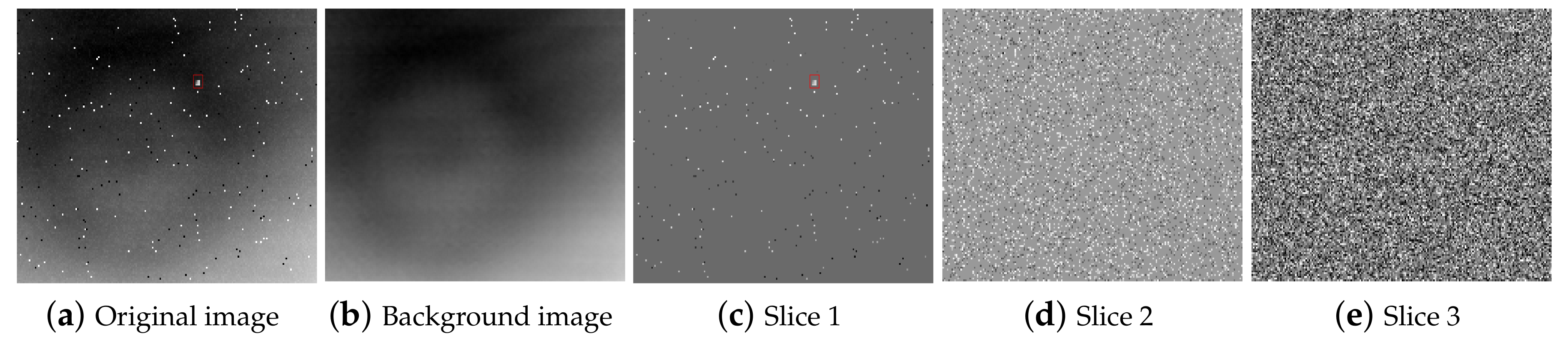
| Step 4: Noise component by . Decompose into K components by Equation (21), and reconstruct noise components into the corresponding image sequences by method in Section 2.1. |
| Step 5: Select the true target images by Equation (22). |
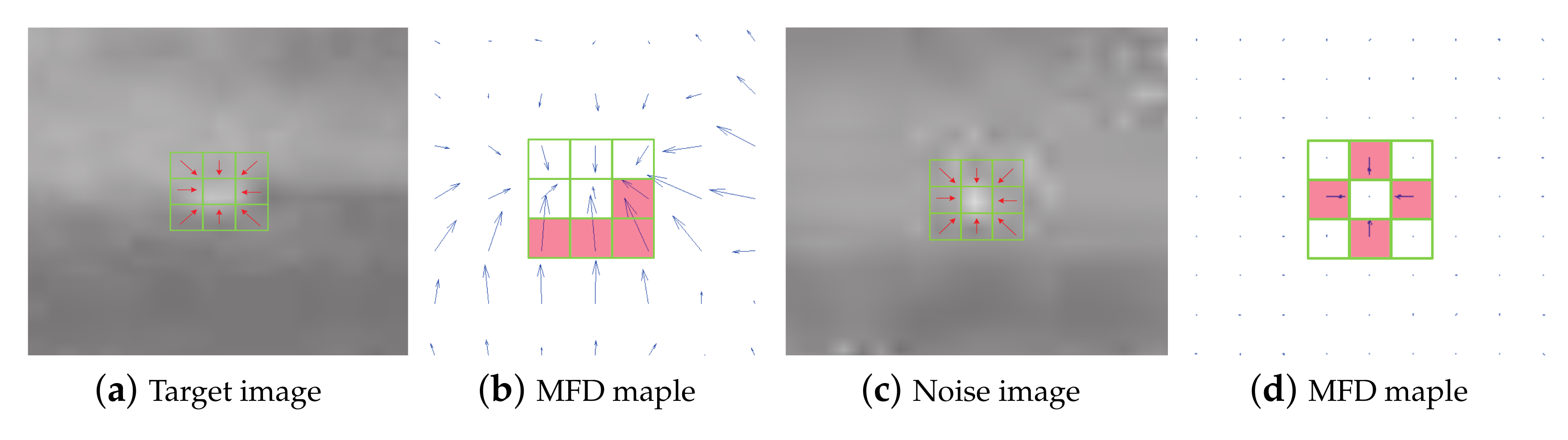
| Step 6: Calculate the original MFD map of the target images by Equations (23) and (24). |
| Step 7: Obtain the separated target images by using both MFD maple and adaptive threshold, which can be computed by Equation (27). |
| Output: Separated target image sequence. |
3. Experiments
3.1. Metrics and Comparative Methods
3.2. Simulated and Real Datasets
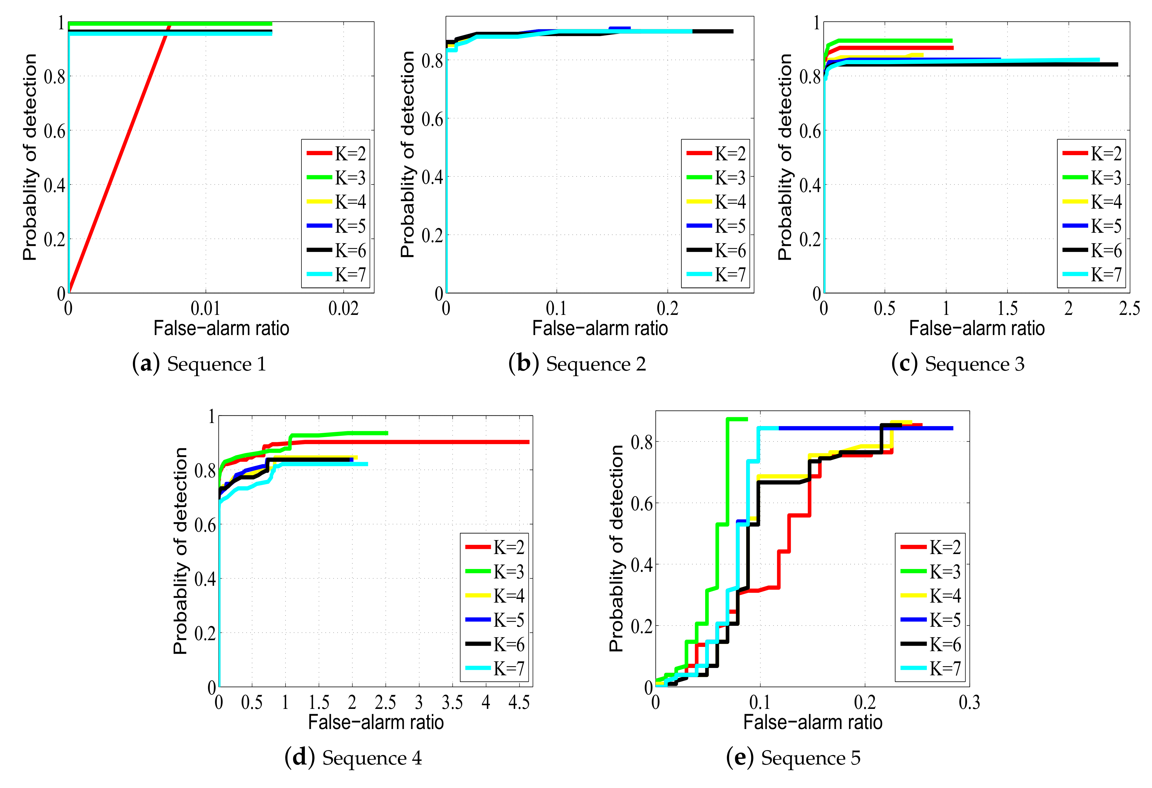
3.3. Effect of Component Number
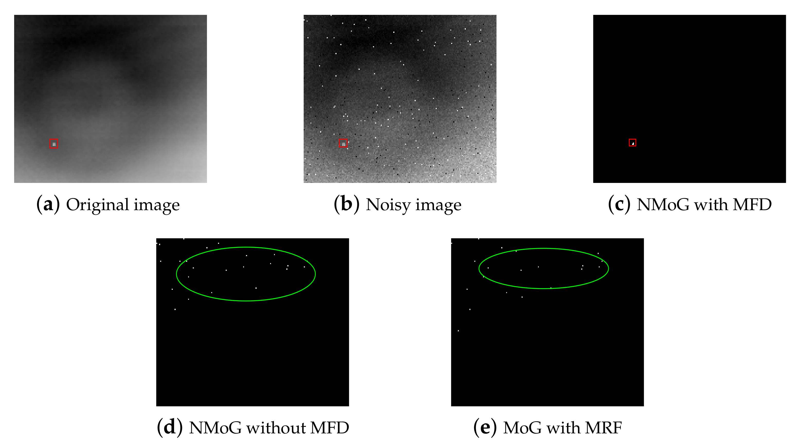
3.4. Effect of MFD
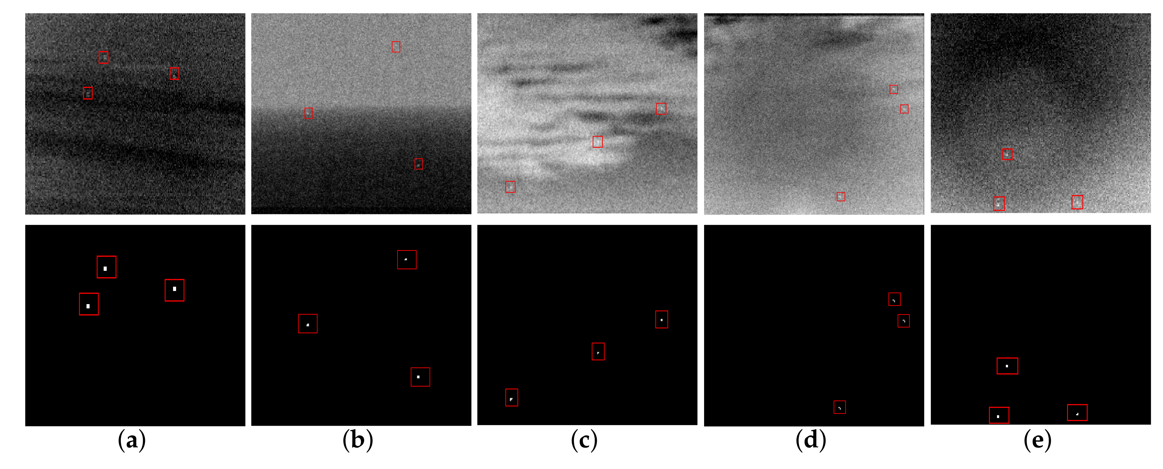
3.5. Performance of Multiple Targets Scene
3.6. Comparisons to Baseline Methods
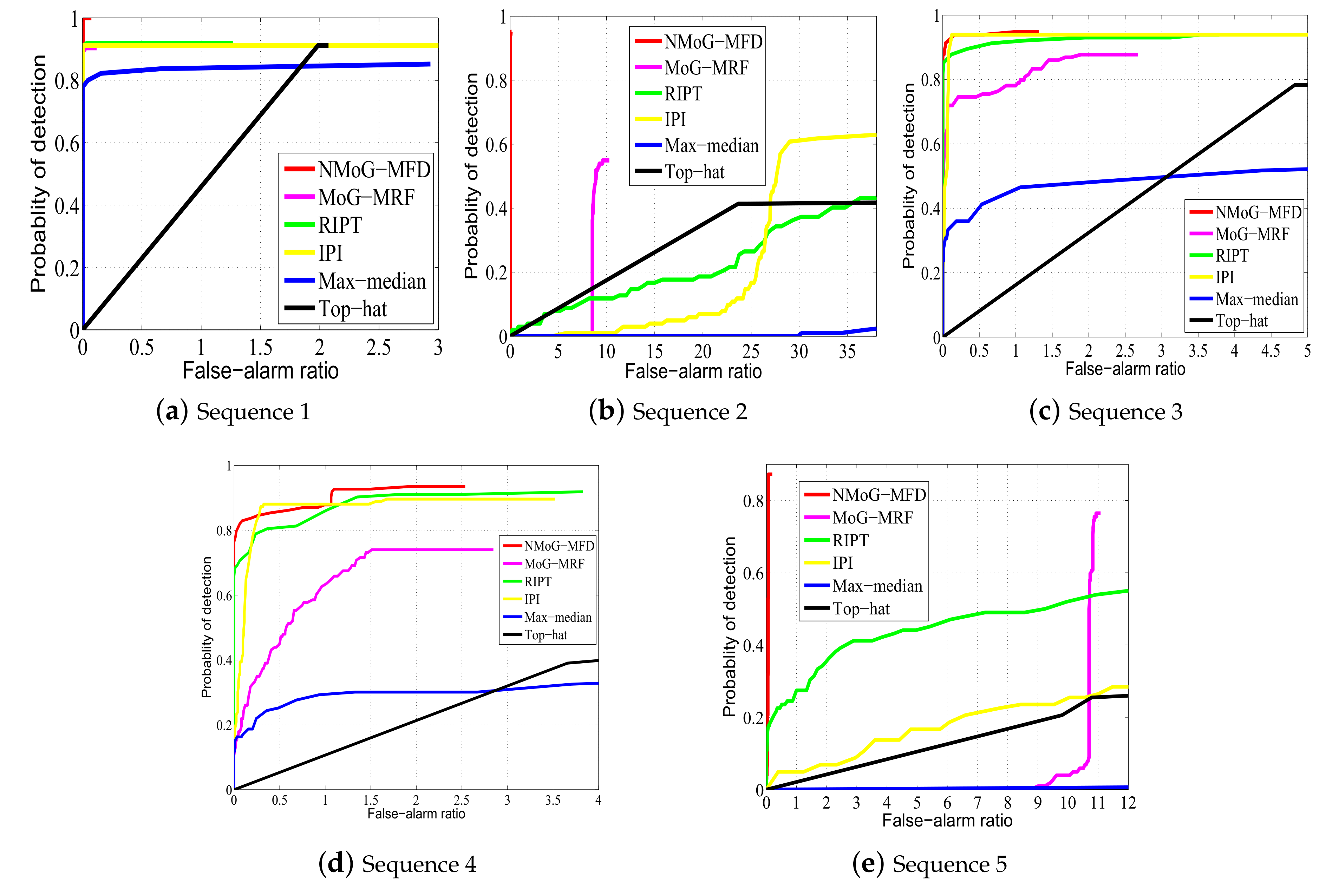
3.6.1. Experiments on Simulated Data
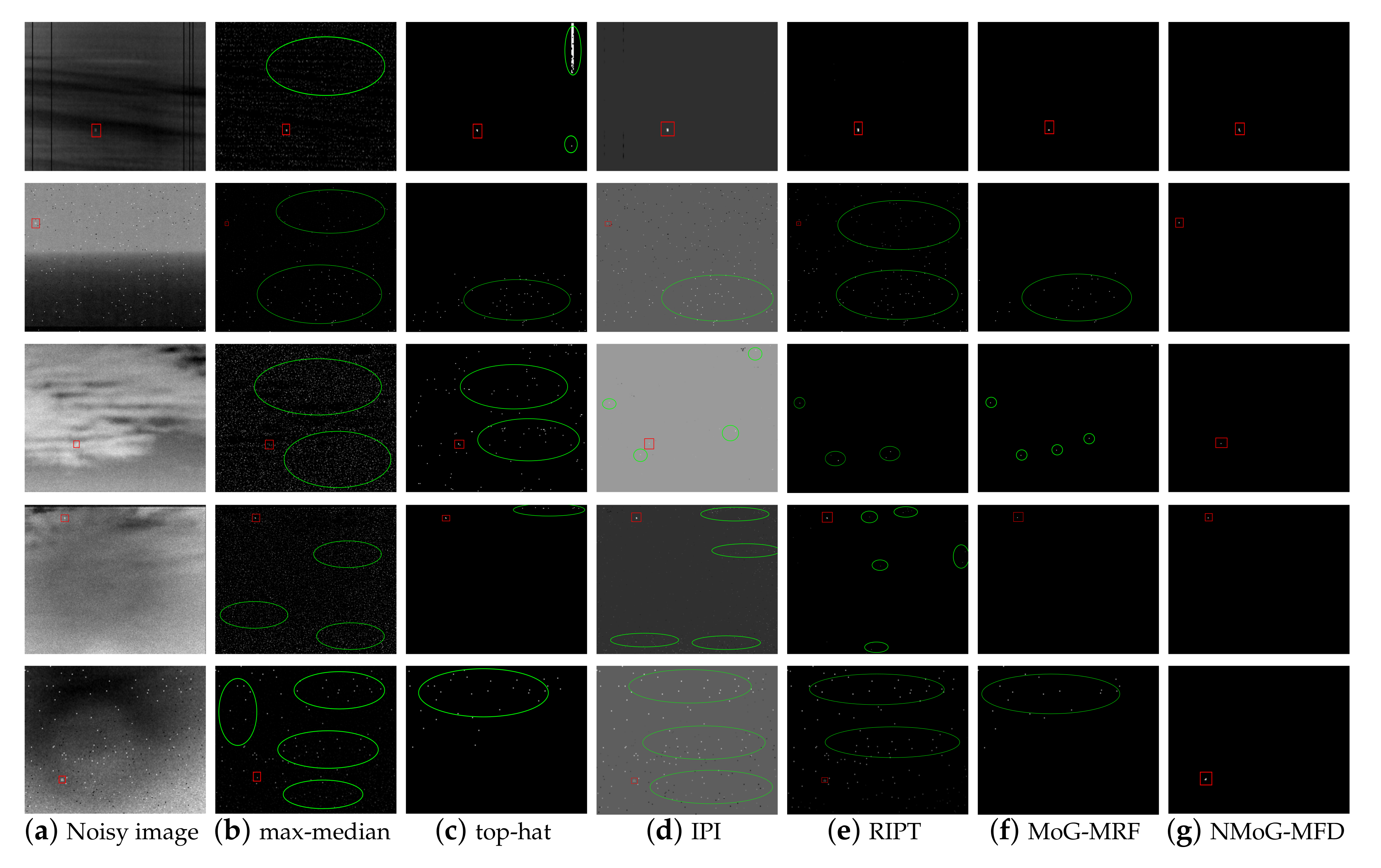
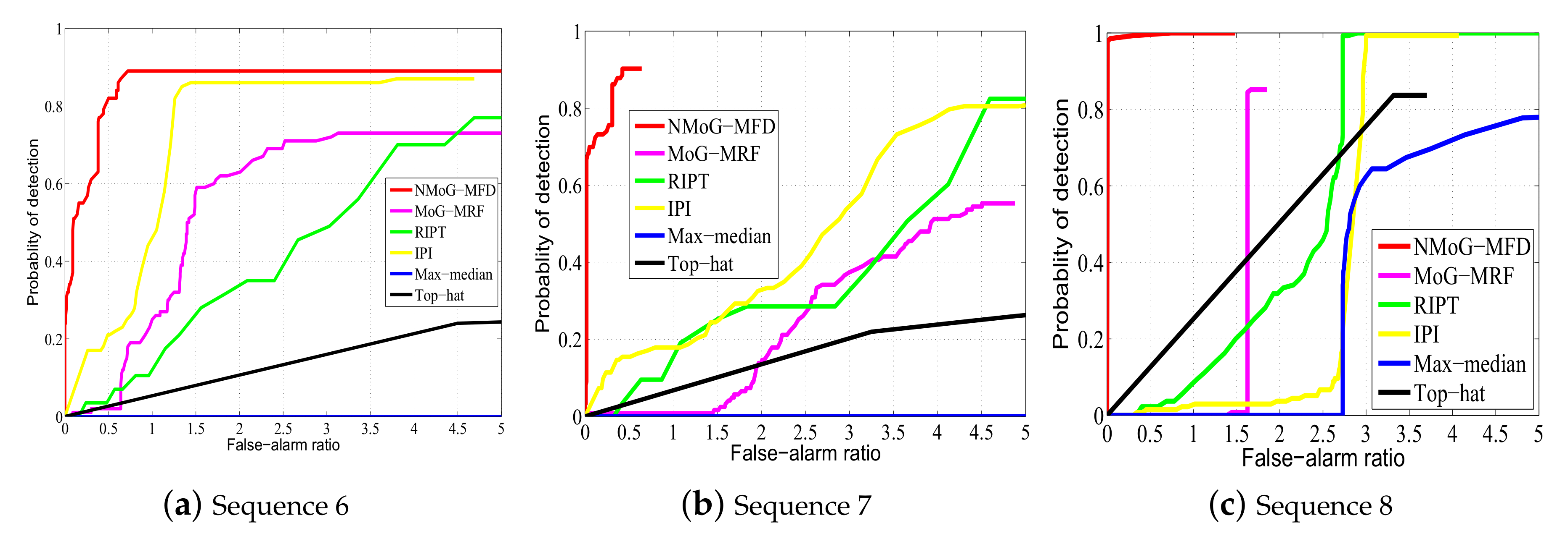
3.6.2. Experiments on Real Data
3.7. Complexity Analysis
4. Conclusions
Author Contributions
Funding
Conflicts of Interest
References
- Chen, Y.; Xin, Y. An Efficient Infrared Small Target Detection Method Based on Visual Contrast Mechanism. IEEE Geosci. Remote Sens. Lett. 2016, 13, 962–966. [Google Scholar] [CrossRef]
- Bai, X.; Chen, Z.; Zhang, Y.; Liu, Z.; Lu, Y. Infrared Ship Target Segmentation Based on Spatial Information Improved FCM. IEEE Trans. Cybern. 2016, 46, 3259–3271. [Google Scholar] [CrossRef] [PubMed]
- Deng, H.; Sun, X.; Liu, M.; Ye, C.; Zhou, X. Entropy-based window selection for detecting dim and small infrared targets. Pattern Recognit. 2017, 61, 66–77. [Google Scholar] [CrossRef]
- Chen, H.; Bar-Shalom, Y.; Pattipati, K.R.; Kirubarajan, T. MDL approach for multiple low observable track initiation. IEEE Trans. Aerosp. Electron. Syst. 2002, 39, 862–882. [Google Scholar] [CrossRef]
- Grossi, E.; Lops, M. Sequential Along-Track Integration for Early Detection of Moving Targets. IEEE Trans. Signal Process. 2008, 56, 3969–3982. [Google Scholar] [CrossRef]
- Li, Y.; Liang, S.; Bai, B.; Feng, D. Detecting and tracking dim small targets in infrared image sequences under complex backgrounds. Multimed. Tools Appl. 2014, 71, 1179–1199. [Google Scholar] [CrossRef]
- Liu, Z.; Zhou, F.; Chen, X.; Bai, X.; Sun, C. Iterative infrared ship target segmentation based on multiple features. Pattern Recognit. 2014, 47, 2839–2852. [Google Scholar] [CrossRef]
- Han, J.; Ma, Y.; Huang, J.; Mei, X.; Ma, J. An Infrared Small Target Detecting Algorithm Based on Human Visual System. IEEE Geosci. Remote Sens. Lett. 2016, 13, 452–456. [Google Scholar] [CrossRef]
- Reed, I.S.; Gagliardi, R.M.; Stotts, L.B. Optical moving target detection with 3D matched filtering. IEEE Trans. Aerosp. Electron. Syst. 2002, 24, 327–336. [Google Scholar] [CrossRef]
- Yang, W.; Sun, X. Moving weak point target detection and estimation with three-dimensional double directional filter in IR cluttered background. Opt. Eng. 2005, 44, 107007. [Google Scholar]
- Liu, X.; Zuo, Z. A Dim Small Infrared Moving Target Detection Algorithm Based on Improved Three-Dimensional Directional Filtering. In Advances in Image and Graphics Technologies; Springer: Berlin/Heidelberg, Germany, 2013; Volume 363, pp. 102–108. [Google Scholar]
- Venkateswarlu, R. Max-mean and max-median filters for detection of small targets. Proc. SPIE Int. Soc. Opt. Eng. 1999, 3809, 74–83. [Google Scholar]
- Fortin, R. Detection of dim targets in digital infrared imagery by morphological image processing. Opt. Eng. 1996, 35, 1886–1893. [Google Scholar]
- Hadhoud, M.M.; Thomas, D.W. The two-dimensional adaptive LMS (TDLMS) algorithm. Circuits Syst. IEEE Trans. 1988, 35, 485–494. [Google Scholar] [CrossRef]
- Kim, S.; Yang, Y.; Lee, J.; Park, Y. Small Target Detection Utilizing Robust Methods of the Human Visual System for IRST. J. Infrared Millim. Terahertz Waves 2009, 30, 994–1011. [Google Scholar] [CrossRef]
- Chen, C.L.P.; Li, H.; Wei, Y.; Xia, T.; Tang, Y.Y. A Local Contrast Method for Small Infrared Target Detection. IEEE Trans. Geosci. Remote Sens. 2013, 52, 574–581. [Google Scholar] [CrossRef]
- Han, J.; Ma, Y.; Zhou, B.; Fan, F.; Liang, K.; Fang, Y. A Robust Infrared Small Target Detection Algorithm Based on Human Visual System. IEEE Geosci. Remote Sens. Lett. 2014, 11, 2168–2172. [Google Scholar]
- Tun, H.U.; Zhao, J.J.; Yuan, C.; Wang, F.L.; Jie, Y. Infrared Small Target Detection Based on Saliency and Principle Component Analysis. J. Infrared Millim. Waves 2010, 29, 303–306. [Google Scholar]
- Wang, C.; Qin, S. Adaptive detection method of infrared small target based on target-background separation via robust principal component analysis. Infrared Phys. Technol. 2015, 69, 123–135. [Google Scholar] [CrossRef]
- Bi, Y.; Bai, X.; Jin, T.; Guo, S. Multiple Feature Analysis for Infrared Small Target Detection. IEEE Geosci. Remote Sens. Lett. 2017, 14, 1333–1337. [Google Scholar] [CrossRef]
- Guangcan, L.; Zhouchen, L.; Shuicheng, Y.; Ju, S.; Yong, Y.; Yi, M. Robust recovery of subspace structures by low-rank representation. IEEE Trans. Pattern Anal. Mach. Intell. 2013, 35, 171–184. [Google Scholar]
- Gao, C.; Meng, D.; Yang, Y.; Wang, Y.; Zhou, X.; Hauptmann, A.G. Infrared Patch-Image Model for Small Target Detection in a Single Image. IEEE Trans. Image Process. 2013, 22, 4996–5009. [Google Scholar] [CrossRef] [PubMed]
- Candès, E.J.; Tao, T. The Power of Convex Relaxation: Near-optimal Matrix Completion. IEEE Trans. Inf. Theor. 2010, 56, 2053–2080. [Google Scholar] [CrossRef]
- Mohimani, H.; Babaie-Zadeh, M.; Jutten, C. A fast approach for overcomplete sparse decomposition based on smoothed L0 norm. IEEE Trans. Signal Process. 2008, 57, 289–301. [Google Scholar] [CrossRef]
- Dai, Y.; Wu, Y.; Song, Y. Infrared small target and background separation via column-wise weighted robust principal component analysis. Infrared Phys. Technol. 2016, 77, 421–430. [Google Scholar] [CrossRef]
- Dai, Y.; Wu, Y.; Song, Y.; Guo, J. Non-negative infrared patch-image model: Robust target-background separation via partial sum minimization of singular values. Infrared Phys. Technol. 2017, 81, 182–194. [Google Scholar] [CrossRef]
- Guo, J.; Wu, Y.; Dai, Y. Small target detection based on reweighted infrared patch-image model. IET Image Process. 2018, 12, 70–79. [Google Scholar] [CrossRef]
- Dai, Y.; Wu, Y. Reweighted Infrared Patch-Tensor Model With Both Nonlocal and Local Priors for Single-Frame Small Target Detection. IEEE J. Sel. Top. Appl. Earth Obs. Remote Sens. 2017, 10, 3752–3767. [Google Scholar] [CrossRef]
- Liu, J.; Musialski, P.; Wonka, P.; Ye, J. Tensor completion for estimating missing values in visual data. IEEE Trans. Pattern Anal. Mach. Intell. 2013, 35, 208–220. [Google Scholar] [CrossRef]
- Sun, Y.; Yang, J.; Long, Y.; Shang, Z.; An, W. Infrared Patch-Tensor Model With Weighted Tensor Nuclear Norm for Small Target Detection in a Single Frame. IEEE Access 2018, 6, 76140–76152. [Google Scholar] [CrossRef]
- Shabalin, A.A.; Nobel, A.B. Reconstruction of a low-rank matrix in the presence of Gaussian noise. J. Multivar. Anal. 2013, 118, 67–76. [Google Scholar] [CrossRef]
- Gao, C.; Wang, L.; Xiao, Y.; Zhao, Q.; Meng, D. Infrared Small-dim Target Detection Based on Markov Random Field Guided Noise Modeling. Pattern Recognit. 2017, 76, 463–475. [Google Scholar] [CrossRef]
- Meng, D.; Torre, F.D.L. Robust Matrix Factorization with Unknown Noise. In Proceedings of the 2013 IEEE International Conference on Computer Vision, Sydney, Australia, 1–8 December 2013; pp. 1337–1344. [Google Scholar]
- Cao, X.; Zhao, Q.; Meng, D.; Chen, Y.; Xu, Z. Robust Low-Rank Matrix Factorization Under General Mixture Noise Distributions. IEEE Trans Image Process 2016, 25, 4677–4690. [Google Scholar] [CrossRef] [PubMed]
- Zhao, Q.; Meng, D.; Xu, Z.; Zuo, W.; Zhang, L. Robust principal component analysis with complex noise. In Proceedings of the 31st International Conference on Machine Learning (ICML 2014), Beijing, China, 21–26 June 2014; pp. 55–63. [Google Scholar]
- Chen, Y.; Cao, X.; Zhao, Q.; Meng, D.; Xu, Z. Denoising Hyperspectral Image With Non-i.i.d. Noise Structure. IEEE Trans. Cybern. 2017, 48, 1054–1066. [Google Scholar] [CrossRef] [PubMed]
- Liu, D.; Cao, L.; Li, Z.; Liu, T.; Che, P. Infrared Small Target Detection Based on Flux Density and Direction Diversity in Gradient Vector Field. IEEE J. Sel. Top. Appl. Earth Obs. Remote. Sens. 2018, 11, 2528–2554. [Google Scholar] [CrossRef]
- Babacan, S.D.; Luessi, M.; Molina, R.; Katsaggelos, A.K. Sparse Bayesian Methods for Low-Rank Matrix Estimation. IEEE Trans. Signal Process. 2012, 60, 3964–3977. [Google Scholar] [CrossRef]
- Bishop, C.M.; Nasrabadi, N.M. Pattern Recognition and Machine Learning; Springer: New York, NY, USA, 2006; p. 049901. [Google Scholar]
- Gao, C.; Zhang, T.; Li, Q. Small infrared target detection using sparse ring representation. IEEE Aerosp. Electron. Syst. Mag. 2012, 27, 21–30. [Google Scholar]


| Methods | Acronyms | Parameter Settings |
|---|---|---|
| max-median filter | max-median | Support size: |
| top-hat method | top-hat | Structure shape: Square, structure size: |
| Infrared Patch-Image Mode | IPI | Patch size: , sliding step: 10, , , |
| Reweighted Infrared Patch-Tensor Model | RIPT | Patch size: , sliding step: 10, , , , |
| Mixture of Gaussians with Markov random field | MoG with MRF | Noise component number: |
| Mixture of Non-i.i.d. Gaussians with Modified Flux Density | NMoG with MFD | Noise component number: |
| Sequence | Number of Frames | Image Resolution (pixels) | Noise Characteristics | Background Characteristics | SCR | |
|---|---|---|---|---|---|---|
| 1 | 135 | Gaussian + Deadline Noise | Sea-Sky Clutters | 0.25∼10.11 | 3.49 | |
| 2 | 108 | Gaussian + Salt and Pepper Noise | Heavy cloud-sky clutters | 0.13∼8.24 | 2.71 | |
| 3 | 114 | Gaussian + Poisson Noise | Heavy cloud-sky clutters | 0.11∼3.30 | 1.33 | |
| 4 | 123 | Gaussian + Impulse Noise | Heavy cloud-sky clutters | 0.02∼4.32 | 1.90 | |
| 5 | 102 | Mixture Noise | Heavy cloud-sky clutters | 0.05∼10.24 | 3.09 |
| Metric | K | Sequence 1 | Sequence 2 | Sequence 3 | Sequence 4 | Sequence 5 |
|---|---|---|---|---|---|---|
| = 0.01/image | = 0.1/image | = 0.5/image | = 2/image | = 0.25/image | ||
| 2 | 0.98 | 0.90 | 0.90 | 0.90 | 0.85 | |
| 3 | 1.00 | 0.90 | 0.94 | 0.93 | 0.87 | |
| 4 | 0.96 | 0.90 | 0.87 | 0.85 | 0.86 | |
| 5 | 0.96 | 0.90 | 0.86 | 0.84 | 0.80 | |
| 6 | 0.96 | 0.89 | 0.84 | 0.84 | 0.81 | |
| 7 | 0.96 | 0.89 | 0.85 | 0.82 | 0.80 |
| 31st Frame of Sequence 1 | 3rd Frame of Sequence 2 | 41st Frame of Sequence 3 | |||||||
|---|---|---|---|---|---|---|---|---|---|
| Method | LSNRG | BSF | SCRG | LSNRG | BSF | SCRG | LSNRG | BSF | SCRG |
| Max-Meidan | 1.6209 | 14.8329 | 2.7474 | 0.4829 | 7.0193 | 3.6076 | 0.4640 | 14.4141 | 0.0792 |
| top-hat | Inf | Inf | Inf | Miss | Miss | Miss | 1.0311 | 2.3991 | 0.2823 |
| IPI | 4.1182 | 1.5731 | 6.207 | 0.976 | 1.5658 | 0.6981 | 0.9828 | 1.3869 | 0.2679 |
| RIPT | Inf | Inf | Inf | 0.6207 | 6.4585 | 13.3034 | 0 | 6.0941 | 32.9413 |
| MoG-MRF | Inf | Inf | Inf | Miss | Miss | Miss | 0 | 6.8651 | 53.2848 |
| NMoG-MFD | Inf | Inf | Inf | Inf | Inf | Inf | Inf | Inf | Inf |
| 4th Frame of Sequence 4 | 22nd Frame of Sequence 5 | |||||
|---|---|---|---|---|---|---|
| Method | LSNRG | BSF | SCRG | LSNRG | BSF | SCRG |
| Max-Meidan | 1.2486 | 9.5636 | 3.2359 | 0.2618 | 2.4965 | 0.366 |
| top-hat | Inf | Inf | Inf | Miss | Miss | Miss |
| IPI | 2.1088 | 3.8868 | 4.8508 | 0.9329 | 1.3979 | 0.4839 |
| RIPT | Inf | Inf | Inf | 0.6674 | 2.901 | 3.6575 |
| MoG-MRF | Inf | Inf | Inf | Miss | Miss | Miss |
| NMoG-MFD | Inf | Inf | Inf | Inf | Inf | Inf |
| Sequence 1 | Sequence 2 | Sequence 3 | Sequence 4 | Sequence 5 | ||||||
|---|---|---|---|---|---|---|---|---|---|---|
| Method | CG | ABR | CG | ABR | CG | ABR | CG | ABR | CG | ABR |
| Max-Meidan | 2.3312 | 0.9221 | 1.2661 | 0.9457 | 2.4625 | 0.9519 | 1.7005 | 0.868 | 1.4464 | 0.8981 |
| top-hat | 3.8321 | 0.9066 | 5.0661 | 0.9286 | 5.6079 | 0.9398 | 4.1474 | 0.9289 | 3.1628 | 0.9192 |
| IPI | 2.6185 | 0.8601 | 1.5188 | 0.8374 | 1.7097 | 0.9067 | 2.5819 | 0.9447 | 1.8794 | 0.8861 |
| RIPT | 3.1073 | 0.9179 | 3.7042 | 0.9303 | 6.1015 | 0.9423 | 3.0008 | 0.9321 | 2.1123 | 0.8993 |
| MoG-MRF | 4.7533 | 0.9327 | 5.2441 | 0.9700 | 6.3158 | 0.9508 | 4.0663 | 0.9584 | 3.8108 | 0.9435 |
| NMoG-MFD | 4.7798 | 0.9801 | 5.6895 | 0.9841 | 8.1627 | 0.9837 | 5.1757 | 0.9849 | 3.8432 | 0.9825 |
| Metric | Methods | Sequence 1 | Sequence 2 | Sequence 3 | Sequence 4 | Sequence 5 |
|---|---|---|---|---|---|---|
| = 1/image | = 15/image | = 2.5/image | = 2/image | = 11/image | ||
| max-median | 0.84 | 0 | 0.49 | 0.30 | 0 | |
| Top-hat | 0.46 | 0.28 | 0.41 | 0.22 | 0.26 | |
| IPI | 0.91 | 0.05 | 0.93 | 0.90 | 0.27 | |
| RIPT | 0.91 | 0.17 | 0.93 | 0.91 | 0.54 | |
| MoG-MRF | 0.90 | 0.52 | 0.88 | 0.74 | 0.75 | |
| NMoG-MFD | 1.00 | 0.90 | 0.94 | 0.93 | 0.87 |
| Metric | Methods | Sequence 6 | Sequence 7 | Sequence 8 |
|---|---|---|---|---|
| = 2/image | = 2/image | = 2/image | ||
| max-median | 0 | 0 | 0 | |
| Top-hat | 0.11 | 0.14 | 0.51 | |
| IPI | 0.86 | 0.33 | 0.04 | |
| RIPT | 0.34 | 0.28 | 0.32 | |
| MoG-MRF | 0.63 | 0.14 | 0.85 | |
| NMoG-MFD | 0.89 | 0.90 | 1.00 |
| Method | Complexity | Times(s) |
|---|---|---|
| max-median | 392.997661 | |
| top-hat | 2.639046 | |
| IPI | 682.764355 | |
| RIPT | 224.866089 | |
| MoG-MRF | 3002.7214 | |
| NMoG-MFD | 482.9220 |
© 2019 by the authors. Licensee MDPI, Basel, Switzerland. This article is an open access article distributed under the terms and conditions of the Creative Commons Attribution (CC BY) license (http://creativecommons.org/licenses/by/4.0/).
Share and Cite
Sun, Y.; Yang, J.; Li, M.; An, W. Infrared Small-Faint Target Detection Using Non-i.i.d. Mixture of Gaussians and Flux Density. Remote Sens. 2019, 11, 2831. https://doi.org/10.3390/rs11232831
Sun Y, Yang J, Li M, An W. Infrared Small-Faint Target Detection Using Non-i.i.d. Mixture of Gaussians and Flux Density. Remote Sensing. 2019; 11(23):2831. https://doi.org/10.3390/rs11232831
Chicago/Turabian StyleSun, Yang, Jungang Yang, Miao Li, and Wei An. 2019. "Infrared Small-Faint Target Detection Using Non-i.i.d. Mixture of Gaussians and Flux Density" Remote Sensing 11, no. 23: 2831. https://doi.org/10.3390/rs11232831
APA StyleSun, Y., Yang, J., Li, M., & An, W. (2019). Infrared Small-Faint Target Detection Using Non-i.i.d. Mixture of Gaussians and Flux Density. Remote Sensing, 11(23), 2831. https://doi.org/10.3390/rs11232831