Article

Self-Training Classification Framework with Spatial-Contextual Information for Local Climate Zones

1
The State Key Laboratory of Information Engineering in Surveying, Mapping and Remote Sensing, Wuhan University, Wuhan 430079, China
2
Hubei Provincial Engineering Research Center of Natural Resources Remote Sensing Monitoring, Wuhan University, Wuhan 430079, China
3
College of Computer Science, China University of Geosciences, Wuhan 430074, China
4
School of Printing and Packing, Wuhan University, Wuhan 430079, China
*
Author to whom correspondence should be addressed.
Remote Sens. 2019, 11(23), 2828; https://doi.org/10.3390/rs11232828
Submission received: 11 October 2019 / Revised: 17 November 2019 / Accepted: 26 November 2019 / Published: 28 November 2019
(This article belongs to the Special Issue Application of Remote Sensing in Urban Climatology)

Abstract

:
Local climate zones (LCZ) have become a generic criterion for climate analysis among global cities, as they can describe not only the urban climate but also the morphology inside the city. LCZ mapping based on the remote sensing classification method is a fundamental task, and the protocol proposed by the World Urban Database and Access Portal Tools (WUDAPT) project, which consists of random forest classification and filter-based spatial smoothing, is the most common approach. However, the classification and spatial smoothing lack a unified framework, which causes the appearance of small, isolated areas in the LCZ maps. In this paper, a spatial-contextual information-based self-training classification framework (SCSF) is proposed to solve this LCZ classification problem. In SCSF, conditional random field (CRF) is used to integrate the classification and spatial smoothing processing into one model and a self-training method is adopted, considering that the lack of sufficient expert-labeled training samples is always a big issue, especially for the complex LCZ scheme. Moreover, in the unary potentials of CRF modeling, pseudo-label selection using a self-training process is used to train the classifier, which fuses the regional spatial information through segmentation and the local neighborhood information through moving windows to provide a more reliable probabilistic classification map. In the pairwise potential function, SCSF can effectively improve the classification accuracy by integrating the spatial-contextual information through CRF. The experimental results prove that the proposed framework is efficient when compared to the traditional mapping product of WUDAPT in LCZ classification.

Graphical Abstract

1. Introduction

The local climate zone (LCZ) scheme is a novel climate-based classification scheme [1], which skillfully relates the urban climate represented by physical traits with urban morphology depicted through landscape cover. The LCZ scheme has the potential to be accepted as a standard description for worldwide cities [2], since its strong performance in indicating the diversity inside cities is also important for urban study. It has been widely used in various fields, such as a series of studies of the urban heat island (UHI) effect [3,4], which adopted the LCZ scheme rather than the traditional dichotomic urban or rural regions to analyze the effects of urban heat islands, making the study of thermal phenomena more specific. The LCZ scheme has also been found to be superior in portraying urban morphology [5,6], where researchers have developed climate-sensitive urban planning strategies aimed at preventing the acceleration of local urban warming. Other fields such as weather forecasting [7], urban health studies [8], and urban energy studies [9] have also shown much interest in the LCZ scheme. It seems that the LCZ scheme is now playing a more and more important role in global urban studies. To better apply the LCZ scheme in urban studies, generating effective and precise LCZ maps is a fundamental problem. There are three main methods used in LCZ mapping: (1) on-site observation; (2) geographic information system (GIS)-based methods; and (3) remote-sensing-based methods [10]. On-site observation requires professional instruments and the related knowledge and is thus not only time-consuming but also difficult for the layperson [11]. The GIS-based methods employ urban-related databases to calculate the relevant LCZ properties [12,13]. This approach can perform well in a specific city but is difficult to duplicate in other areas; moreover, the acquisition of GIS data is often difficult, which limits further application [14]. As a result, remote-sensing-based methods are now in common use.
The remote-sensing-based LCZ methods combined with Earth observation data such as Landsat and Sentinel images have the potential to map global cities. Considering this fact, an initiative called the World Urban Database and Access Portal Tools (WUDAPT) project [15,16] adopted the LCZ scheme to produce its city-level data (level 0 data), using LCZ classification to delineate the coarse urban morphology. This project proposed an LCZ mapping method for the publicly available Landsat images, which outperformed random forest (RF) classification [17] on the Google Earth and System for Automated Geoscientific Analyses (SAGA) [18] platforms. Since the patches in the obtained maps are too fragmented due to the LCZ concept, majority-filter-based spatial smoothing is added into the final protocol to generate smoother results. Hence, RF classification and the majority filter make up the official WUDAPT pixel-based LCZ mapping workflow [19]. This approach has been widely used in a number of studies. Demuzere et al. [20] adopted this protocol to generate a continental-scale LCZ map of Europe; Bechtel et al. [21] analyzed the surface urban heat island (SUHI)effect among 50 cities from the outcome of WUDAPT; and Shi et al. [22] used this LCZ classification scheme to assist in urban air quality study. Nevertheless, although the well-known WUDAPT LCZ mapping method introduces the majority filter to mitigate the fragmented pixels, the results are still unsatisfactory when using only the spatial neighborhood information. This results in the appearance of small, isolated misclassified areas, which can be solved by considering the spatial-contextual information. Given this fact, three kinds of improved methods have been developed to date. The first method is the object-oriented LCZ classification approaches [23,24], which use segmentation regions rather than a single pixel as the processing unit. However, the classification is seriously influenced by the segmentation scale, which inadvertently brings a new problem, i.e., how to choose the optimal scale. The second type of method is based on the spatial-smoothing-based LCZ approach with Markov random fields (MRF) [25]. This method not only can integrate the spatial-contextual information but also avoids the selection of the optimal scale, whereas MRF only considers the spatial-contextual information among the labels and ignores the original samples. The third is the deep-learning-based LCZ classification methods [26,27,28], which use convolutional and pooling layers to capture spatial-contextual information and to improve the performance of classification. While the utilization of spatial-contextual information depends on the depth of the network, a shallow net usually considers the regional area and a deep net considers global area, which makes the elaborate configuration of the network become another issue.
In this paper, to comprehensively solve these problems, a spatial-contextual information-based self-training classification framework for LCZs (SCSF) is proposed. In SCSF, the spatial-contextual information can be directly integrated into the classification step with the flexible ability of conditional random fields (CRF), which models the spatial-contextual information in both the samples and the corresponding labels with a strong theoretical basis. CRF has been widely used in image segmentation [29,30] and image classification [31,32,33,34], and although CRF has a powerful modeling ability for spatial-contextual information, when it comes to LCZ classification, the small number of expert-labeled samples directly impacts the quality of the probabilistic classification map, resulting in unreliable inputs for modeling the potential function in CRF. Considering this fact, we propose an improved self-training method with spatial information-based pseudo-label selection to provide a more reliable probabilistic classification map. The proposed SCSF method can help to prevent the appearance of fragmented pixels, and better predictions can be obtained with the integration of the classification and spatial-contextual information. The main contributions of this paper are as follows:
  • The spatial-contextual information based self-training classification framework for LCZs. Considering that the traditional remote-sensing-based LCZ mapping approaches separate the classification and the spatial smoothing into two independent components, which causes the small, isolated areas in LCZ maps, the proposed SCSF method adopts CRF to directly integrate the spatial-contextual information into the classification with a unified theoretical basis. In addition, an improved self-training method is used to mitigate the conflict between the shortage of expert-labeled LCZ samples and the reliable probabilistic classification maps, serving as inputs for CRF. With the help of spatial-contextual information-based pseudo-label selection, the improved self-training method is able to iteratively enrich the training set and to retrain the classifier, which can provide a more confident probabilistic classification map.
  • Conditional random fields (CRF) for LCZ classification.
    The traditional classifiers consider each pixel independently, without considering the correlation between neighbors, which causes the appearance of salt-and-pepper noise. Although the filter-based spatial smoothing uses spatial constraints to mitigate this problem, the small, isolated areas still remain due to the lack of a unified framework between the classification and spatial smoothing steps. Given this fact, a spatial-contextual information-based method—CRF—is applied to describe the relationship between the samples and labels through the unary potentials and it simultaneously models the spatial correlation between the labeled and observed data by the pairwise potentials. With the hypothesis that the neighboring pixels in homogeneous regions usually have the same label, pairwise CRF-based classification can help to capture the spatial-contextual information, which is important for LCZ mapping, and can thus present a smoother classification map.
  • Probabilistic classification with self-training.
    Although CRF has a flexible modeling ability for spatial-contextual information, the potential function requires a reliable probabilistic classification map. Consider that the quality of the probabilistic classification map is seriously affected by the small training set; a self-training method is introduced, in which a pseudo-label selection strategy using the regional information among the whole image and the local information between neighbors is proposed to identify more confident predictions. With the assumption that similar data in a homogeneous area are more likely to have the same label, self-training with spatial-contextual information-based pseudo-label selection is able to provide a more accurate probabilistic classification map.
The proposed method was tested on three datasets provided as part of the 2017 IEEE Geoscience and Remote Sensing Society (GRSS) Data Fusion Contest. Compared with the WUDAPT method, which uses the RF classifier and spatial smoothing with a majority filter, the proposed method gives an excellent performance. Other methods including Naive Bayes (NB), Support Vector Machine (SVM), and improved WUDAPT approach were also further utilized to compare with the proposed method. Moreover, the LCZ classification framework integrating classification and spatial-contextual information is effective even with limited data.

2. Methodology

2.1. The World Urban Database and Access Portal Tools (WUDAPT) Project

LCZs are defined as regions representing horizontal distances of hundreds of meters to several kilometers with uniform surface cover, structure, materials, and human activity [1]. The LCZ scheme focuses on the land surface temperature between 1.2–1.5 m above ground, which is greatly influenced by the landscape factors. In total, 17 different culturally neutral landscape types, including 10 built types and 7 land-cover types, form the standard LCZ scheme, which is shown in Figure 1. Each type is related to two kinds of climate-sensitive indicators: qualitative indicators and quantitative physical properties. The detailed units better depict the diversity and complexity inside cities, which has led to a revolutionary leap for urban microclimate research [35]. As a result, the LCZ scheme has attracted interest in various fields. The operable supervised LCZ workflow has been published by the World Urban Database and Access Portal Tools (WUDAPT) project, and further study is still in progress.
The WUDAPT project [36,37] is an initiative project for the acquisition, storage, and dissemination of climate-relevant data on the physical traits of global cities. The WUDAPT data collections have three levels: level 0 provides a rough LCZ classification based on remote sensing data; level 1 provides more detailed information on the urban form and function via crowdsourcing techniques; and level 2 is responsible for gathering the finer parameters from these zones. The supervised remote-sensing-based LCZ mapping approach [19] proposed by WUDAPT in Figure 2 has been utilized to collect level 0 data from the crowdsourcing community. With the help of Google Earth and the open-source SAGA GIS software, people without any specific knowledge can also map LCZs through data labeling, supervised classification, and filter-based spatial smoothing steps. Unfortunately, many of the LCZ labeled samples collected via the crowdsourcing community are ambiguous, resulting in a lack of high-quality expert-labeled data, which usually causes an inferior prediction. Thus, a method which is able to perform well in the case of a small number of training samples is required.

2.2. Self-Training Method.

Semi-supervised learning was developed to deal with the limited data issue, and it can help to unlock the potential of huge unlabeled datasets. The self-training approach proposed by Scudder [38] is the earliest semi-supervised method [39], which has been widely used in gene prediction [40], parsing [41], and image classification [42,43] for its simplicity and clarity.
In the traditional self-training method, a base learner is first trained on the original, small, labeled training set and high-probability pseudo-labels are then used to enrich the original labeled set until the learner is retrained and reaches the stopping conditions. The unlabeled data provide extra information to modify the learner, which is usually ignored in the supervised methods, making the description of the model closer to the real distribution of the data. The procedure of a basic self-training method is shown in Figure 3 can be summarized as the following four steps:
Step 1—Initialization: Train the base classifier C i n t on the initial training set ( X t r a i n , y t r a i n ) from the given labeled data ( X l , y l ) .
Step 2—Selection: Predict the data in unlabeled set X u with classifier C i n t , and select the high-probability data ( X c o n f , y c o n f ) as pseudo-labels.
Step 3—Updating: Remove the selected unlabeled samples X c o n f from the unlabeled set X u , and combine the original data ( X l , y l ) with the pseudo-labeled data ( X c o n f , y c o n f ) to update the training set ( X t r a i n , y t r a i n ) ;
Step 4—Retraining: Retrain the classifier C i n t with the updated data ( X t r a i n , y t r a i n ) , and repeat Steps 2–4 until the stopping conditions are satisfied.
However, the traditional self-training method starts the learning from only a few labeled samples, with which it is difficult to capture the clear boundaries between classes, and the mislabeled samples are then brought into the next learning iteration, thereby confusing the classifier. Thus, more powerful pseudo-label selection strategies are urgently needed. Aydav and Minz [44] developed an improved self-training approach using granulation to select the most confident data in a block, rather than a single pixel. Although this approach takes the regional information into account, the confidence obtained from the predicted probability on only a few labels is still low.
Given this fact, in the proposed approach, the commonly used probability is replaced by a strategy considering the spatial-contextual information. After a series of selections from homogenous blocks to candidates and pseudo-labels, the proposed strategy presents a strong performance and provides a preferable probabilistic classification map for CRF.

2.3. The Spatial-Contextual Information-Based Self-Training Classification Framework (SCSF) for Local Climate Zones

Spatial-contextual information has been proved important for LCZ classification [24,45]; however, it is usually independent of the classification step and, without a unified theoretical basis, causes the appearance of small, isolated noise areas. Considering this fact, the proposed spatial-contextual information-based self-training framework (SCSF) introduces the conditional random fields (CRF) and self-training method to provide a better solution. To be specific, CRF is adopted for LCZ classification to integrate the spatial-contextual information directly into the classification by simultaneously modeling the relationship between samples and labels and the spatial correlation among samples and labels, which provides strong theoretical guidance. Furthermore, a probabilistic classification map with the self-training method which is improved by spatial-contextual information-based pseudo-label selection is used for the potential function in CRF by enriching the original labeled dataset with pseudo-labels and by retraining the classifier when the training samples are limited in LCZ mapping.
Firstly, the initial feature space is built with Landsat 8 spectral data and the remote sensing indices of the modified normalized difference water index (MNDWI), the normalized difference vegetation index (NDVI), the ratio vegetation index (RVI), the bare soil index (BSI), the normalized difference building index (NDBI), and the normalized difference impervious surface index (NDISI). After principal component analysis (PCA) transformation, the features are divided into labeled and unlabeled sets, and the labeled data are used to train the base classifier. In the meantime, the efficient graph-based segmentation mask is generated from the input data. Next, the pseudo-labeled samples are selected according to the segmentation and prediction. With the adjustment of the base classifier, the performance is gradually improved and becomes much closer to the specific LCZ scheme. Finally, the CRF models the log-based unary potentials and the edge feature function-based pairwise potentials to simulate the relationship and spatial correlation between samples and labels, which offers a better and smoother prediction. The workflow of the spatial-contextual information-based self-training framework is shown in Figure 4 and is described in the following.

2.3.1. Feature Extraction Based on Multiple Indices

According to the height, compactness, surface cover, and thermal admittance, the LCZ system mixes independent land-cover elements, such as building, tree, farm land, and road, to form unique LCZ types, which leads to an inferior spectral separability, especially for the similar categories. In order to express the characteristics of the LCZ categories, six beneficial remote sensing indices are extracted: MNDWI, NDVI, RVI, BSI, NDBI, and NDISI. The indices are introduced in the following.
The MNDWI [46] is a modified formula for extracting water areas, which is, of course, helpful for LCZ G. Compared with the normalized difference water index (NDWI), the MNDWI changes the original band combination by replacing the near-infrared with the mid-infrared band, which is more effective in distinguishing water information from built-up areas.
The NDVI [47] is a common ratio in vegetation identification, and it is beneficial not only for land-cover types such as LCZ A–D but also for the built types, such as LCZ 1–3. The NDVI can be used to describe the growth of plants, with a value ranging from −1 to 1, where a negative value means high-reflectivity objects and a positive value represents vegetation.
The RVI [48] is sensitive to high-density vegetation and sharply decreases when the vegetation fraction is less than 50%. Green and healthy plants make the RVI much larger than 1, while for land without vegetation, the value is around 1. The RVI has potential for types such as LCZ A–C, as it can reflect the sparseness or density of vegetation.
The BSI [49] is usually used for discriminating bare land from other land covers, such as built-up, water, and vegetation, since the value is much higher in bare land areas. With the help of the near-infrared and mid-infrared bands, the BSI is effective in identifying the soil-related LCZ categories, such as LCZ 7, C, and F.
The NDBI [50] is regarded as a substitute for the building surface fraction (BSF), a ratio of building plan area to total plan area, in 10 LCZ basic physical properties. The NDBI can provide building information through its density, usually denoted by a specific value.
The NDISI [51] introduces the thermal infrared band to differentiate impervious surfaces from soil. Moreover, it has the ability to extract more accurate impervious area information through the restriction of the negative influence of sand and water. The NDISI is used as a replacement for the impervious surface fraction (ISF), a ratio of impervious plan area (paved, rock) to total plan area (%).

2.3.2. Probabilistic Classification with Self-Training

In order to provide a more reliable probabilistic classification map in the case of limited expert-labeled data, a self-training method is considered. Since the spatial-contextual information is important for LCZ classification, it is also used in the improvement of the self-training method. The proposed self-training approach with spatial-contextual information-based pseudo-label selection depends on two main assumptions. The first is that samples with more similar features are more likely to belong to the same category, which is developed by the regional information-based segmentation step. The second is that a pixel surrounded by others with the same label is more reliable, which is achieved through the local information-based candidate identification. The experiments undertaken in this study confirmed that both the regional constraints and the neighborhood information are beneficial for more reliable pseudo-label selection. And the improved self-training method is shown in Figure 5.
1. Segmentation of Features
The Felsenszwalb [52] method in a Python package is used to segment the input features and to generate a segmentation mask, which introduces the regional spatial information to cluster similar features. As a classical image segmentation algorithm, it first computes Felsenszwalb’s efficient graph and then builds a minimum spanning tree. The final segmentation comprehensively considers the internal difference of a component and the difference between two components.
2. The LCZ Base Classifier
After feature extraction, the dataset D is divided into an unlabeled set D u = { X l } and labeled set D l = { X l , y l } , and the latter is further split into a training set D t r a i n = { X t r a i n , y t r a i n } and test set D t e s t = { X t e s t , y t e s t } . The base classifier, RF, is then learned on the training set D t r a i n . RF [53] is a diversity-based ensemble method, and its diversity comes from the various training sets with random samples and features. The randomness in RF comes from the random sample selection, where each base classifier has its own dataset through the bootstrap strategy. Further randomness comes from the random attribute selection, where different features are input to the learning process. The final result is voted for by a group of base classifiers in RF, which provides strong robustness.
There are two reasons for employing the RF classifier. Firstly, RF has an innate advantage in dealing with a small amount of data due to its bootstrap technique, which can enlarge the original database by sampling with the replacement. Secondly, the ensemble strategy, i.e., the majority voting method, makes RF insensitive to noise. One forest includes groups of the base classifier, which are mostly classification and regression trees (CARTs) [54], and each tree is trained on the diverse dataset. Even if misclassification appears in some of the results, the final voting will be stable. Above all, RF is adequate as the base classifier in the case of the label shortage issue.
3. Selection of Candidates
The candidate selection consists of two steps: (1) collecting homogeneous segments and (2) selecting potential samples. A superimposed map with a prediction and segmentation mask is generated at this stage, which puts the regional spatial constraints on the unreliable predictions, i.e., incorporating labels with the input data. According to the first hypothesis introduced previously, i.e., neighboring pixels in homogeneous regions usually have the same label, one block with lots of the same labels is defined as a homogeneous region. The most frequent labels inside the homogeneous block then form the final candidates.
4. Selection of Pseudo-Labels
There are also two procedures used to identify the final pseudo-samples: (1) capturing the 8-neighbor information and (2) sorting the calculated entropy. According to the second assumption mentioned previously, candidates with a lower entropy are likely to be the most useful pseudo-labels.
To be specific, the neighborhood information is captured by a 3 × 3 size moving window. If there are k pixels having the same label among the surrounding 8-neighbors, then the label frequency for each class is defined as follows:
p j i = n = 1 9 k j i n 9
where p j i represents the label frequency of class j for the ith pixel in the candidate set, n is the neighbor of the ith pixel in the 8-neighbor region N, and k j i n denotes if the neighbor n of the ith pixel belongs to the class j.
The label frequency p j i is then used to calculate the entropy as follows:
e i = j = 1 | C | p j i l o g p j i
where e i is the entropy of the ith pixel in the candidate set and | C | represents the number of classes. The entropy captures the certainty of the prediction, with a higher value denoting greater uncertainty.
5. Update and Stopping Condition
The selected pseudo-labels are updated to enrich the original training set, which can offer more information for the base classifier. The latest prediction is then output to the base classifier to assist the new training process. The classifier is gradually modified until a stable classification accuracy is achieved and the final prediction is produced.

2.3.3. Conditional Random Fields (CRF) for LCZ Classification

The majority of the existing LCZ mapping methods separate the classification and the consideration of the spatial-contextual information into independent steps, which causes the appearance of small, isolated noise regions. However, the concept of an LCZ covers hundreds to thousands of meters, which means that the local climate of a very small area is usually discarded. CRF [55] is able to solve this problem by directly bringing the spatial-contextual information into the classification, which also provides a unified theoretical basis for better exploring the spatial-contextual information.
The most common CRF for the image classification task—pairwise CRF [56]—is used to model the spatial dependencies among the 8-neighbors. The energy function E(x) is defined as follows:
E ( x ) = i V ψ i ( x i , y ) + λ i V , j N i ψ i j ( x i , x j , y )
where i is the location of the pixel in the image data V = { 1 , 2 , , K } , K is the total number of images, x i is the label corresponding to the ith pixel, and y is the original input data. ψ i ( x i , y ) and ψ i j ( x i , x j , y ) represent the unary potentials and pairwise potentials, respectively. λ is a nonnegative constant used to trade off the performance of the unary and pairwise potentials. N i represents the local neighborhood of pixel i.
The unary potentials ψ i ( x i , y ) reflect the correlation between the single pixel and the particular label and are defined as follows:
ψ i ( x i , y ) = l n ( P ( x i = l t ) )
where P ( x i = l t ) denotes the probability of x i being labeled as l t , where the probabilistic classification map from the RF classifier is used.
The pairwise potentials ψ i j ( x i , x j , y ) incorporate the spatial-contextual information with the image pixels and labels and model a smoothness prior as follows:
ψ i j ( x i , x j , y ) = { 0 , i f   x i = x j g ( i ,   j ) | | i j 2 | | , o t h e r w i s e
where
g ( i ,   j ) = 1 + θ v e θ w | | x i x j | | 2
where g ( i ,   j ) is an edge feature function measuring the difference among neighbors, the pair of ( i ,   j ) represents the location of neighboring pixels, θ v controls the degree of smoothing, and θ w is designed as the mean-square difference between the spectral vector of adjacent pixels over the whole image.

3. Experimental Results and Discussions

3.1. Experimental Description

To test the performance of the proposed SCSF method, three experiments were conducted, each using two Landsat 8 images and one ground truth provided as part of the 2017 GRSS Data Fusion Contest (2017DFC). The ability of the introduced CRF method to integrate spatial-contextual information was compared with that of two other LCZ mapping methods. The RF classification was used as a baseline, the widely accepted LCZ mapping workflow proposed by WUDAPT (comprising RF classification and majority-filter(MJ)-based spatial smoothing) was used as another reference framework, denoted as RF+MJ(WUDAPT), and the CRF for LCZ classification was denoted as RF+CRF. In addition, to evaluate the capacity of self-training-based probabilistic classification, the proposed, improved self-training method, namely ST, was integrated into the above approaches. The main comparison experiments were finally divided into two parts: supervised methods (i.e., RF, RF+MJ(WUDAPT), and RF+CRF) and semi-supervised method (i.e., RF+ST, RF+ST+MJ, and RF+ST+CRF(SCSF)). Other machine learning classifiers, Naive Bayes (NB) and Support Vector Machine (SVM), which had been widely used in LCZ classification [57,58], were also conducted in this section. Also, the improved WUDAPT method [28,45], denoted as CI-WUDAPT, which considered the contextual characteristics including the mean, minimum, maximum, median, and 25th and 75th quantile values of all pixels in a 3 × 3 window, was also used to compare the performance of the proposed SCSF.
All the experiments were implemented in Python, while the RF classifier was set with 32 estimators and 10 as its maximum depth. The range of the majority filter in the WUDAPT method was a 3 × 3 square window size, and the nonnegative constant λ in CRF was set as 0.5. It is well known that the configurations of the training set and testing set play important roles in the assessment of the LCZ classification [28,45,59]. Since the ground truth data was usually limited, 10 labeled samples were randomly selected in each class for simulating the insufficiency of labeled samples and the remaining samples were used as a testing set, which is widely used in many semi-supervised researches [60,61]. Also, the final experimental results were the average performance of 10 run outcomes for providing better representativeness.
The quantitative performances are assessed by three kinds of accuracies: (1) the accuracy of each class; (2) the overall accuracy (OA), which denotes the percentage of correctly classified samples; and (3) the kappa coefficient (Kappa). Moreover, in order to evaluate the statistical significance of the difference between the proposed algorithms, McNemar’s test [62] was applied under the same classification conditions. Given two classifiers C 1 and C 2 , McNemar’s test can be computed as follows:
X 2 = ( | M 12 M 21 | 1 ) 2 M 12 + M 21
where M 12 represents the number of pixels misclassified by C 1 but not by C 2 and M 21 represents the number of pixels misclassified by C 2 but not by C 1 . If M 12 + M 21 20 , then this statistic can be considered as achi-squared distribution χ 1 2 . McNemar’s test can evaluate whether the difference between the results of two classifiers is significant. Given the common 5% level of significance, then χ 0.05 , 1 2 = 3.841459 . Also, if X 2 is greater than χ 0.05 , 1 2 , then the performances of the two classifiers are significantly different.

3.2. Experimental Results and Analysis

3.2.1. Berlin Experiments

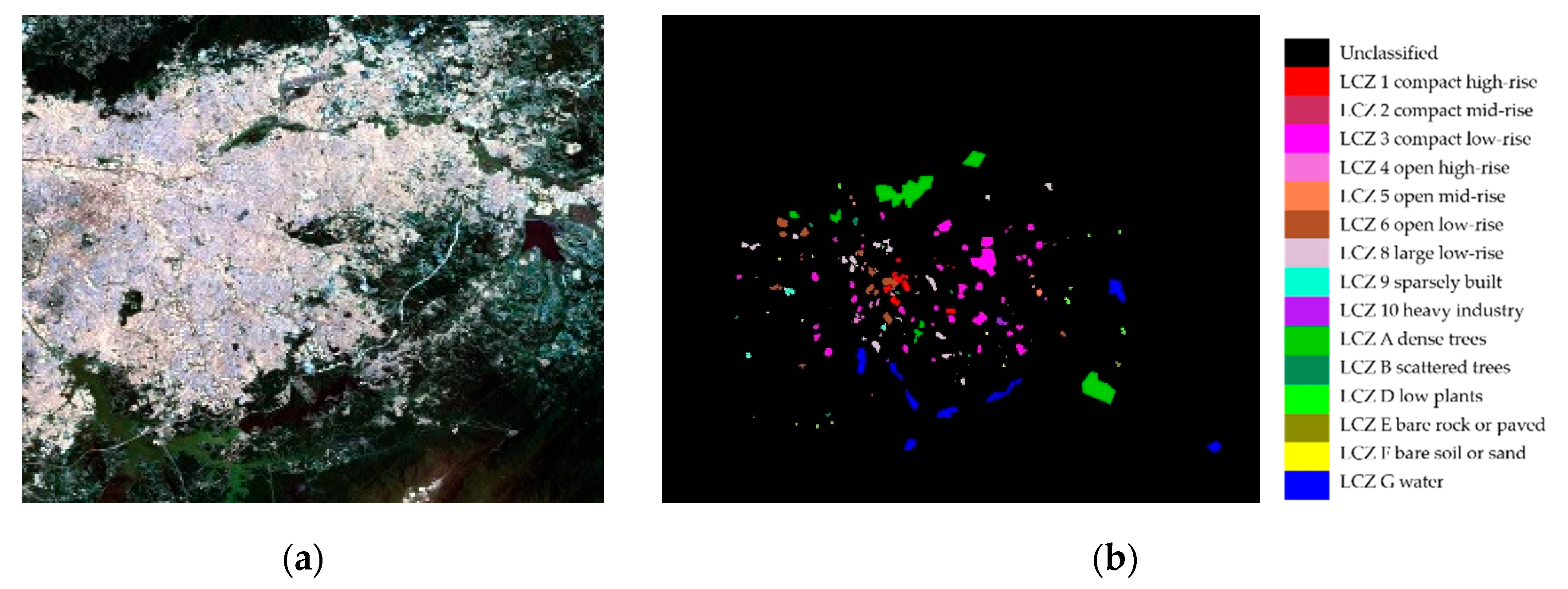
As a city with high attention to urban planning, Berlin in Germany has a balanced urban spatial structure, making itself a model for urban studies. The LCZ types in Berlin are six LCZ built types (i.e., LCZ 2 compact mid-rise, LCZ 4 open high-rise, LCZ 5 open mid-rise, LCZ 6 open low-rise, LCZ 8 large low-rise, and LCZ 9 sparsely built) and six LCZ natural types (i.e., LCZ A dense trees, LCZ B scattered trees, LCZ C bush or scrub, LCZ D low plants, LCZ F bare soil or sand, and LCZ G water). The first experiment was conducted using two down-sampled Landsat 8 images with a 100-m spatial resolution from 2017DFC, which were acquired on 25th March and 10th April 2014. The experimental images contained 666 × 643 pixels, with seven multi-spectral bands (1–7) and two thermal infrared bands (10–11). A false-color image consisting of three bands (Red, green and blue (RGB)) is shown in Figure 6a. The spatial distribution of the corresponding labels is presented in Figure 6b, and the number of labeled samples for each type is given in Table 1. In addition, the training data were randomly sampled from the ground truth for each class.
The LCZ classification maps obtained by the different frameworks (i.e., NB, SVM, CI-WUDAPT, RF, RF+MJ(WUDAPT), RF+CRF, RF+ST, RF+ST+MJ, and RF+ST+CRF(SCSF)) for the Berlin images are displayed in Figure 7a–i, respectively. As the figures show, classification without spatial-contextual information, i.e., RF, presents lots of salt-and-pepper noise. After inputting the spatial constraints from the majority-filter-based spatial smoothing, the other LCZ prediction using the RF+MJ(WUDAPT) workflow produces a smoother LCZ mapping result with a better visual effect. However, the majority filter only considers the narrow neighborhood information given by the predictions, and the small, isolated noise areas remain to be solved. The RF+CRF method generates a much better performance in mitigating the above problem. Nevertheless, misclassification arises from the insufficient training samples, as in area 1 of Figure 7d, where the LCZ F bare soil or sand (yellow) is supposed to be LCZ D low plant (green), which also confuses the CRF modeling, causing the area 1 of Figure 7f (i.e., RF+CRF) to be mislabeled as LCZ F bare soil or sand. Considering this, the semi-supervised self-training methods were then applied to improve the initial predictions. Supported by the enriched training samples from the pseudo-labels, the RF+ST method provides a cleaner map than RF and the comparison between the results of RF+ST+MJ and RF+MJ also reveals the same case. Moreover, area 1 of Figure 7g,h is corrected to LCZ D low plants (green). The RF+ST+CRF(SCSF) workflow exhibits a competitive performance in solving the misclassified noise, with the help of the use of unlabeled data through the improved self-training method and the unified spatial-contextual information-based classification through CRF. Furthermore, results of NB and SVM shown in Figure 7a,b present relatively poor performance with lots of fragile segments. For the prediction of CI-WUDAPT, the smoother boundaries among different classes are presented after the extraction of regional spatial-contextual from features, while heavy misclassified phenomena appeared with the limited training samples (10 samples per class), such as massive LCZ G water (blue) being obviously misclassified to LCZ C bush or scrub (light blue). From the aspect of visual performance, the proposed SCSF delivers the better solution in handling the fragile segments and misclassified areas, which proves the superior capability of the SCSF.
In addition, Table 2 provides the pairwise comparison between the nine methods (i.e., NB, SVM, CI-WUDAPT, RF, RF+MJ(WUDAPT), RF+CRF, RF+ST, RF+ST+MJ, and RF+ST+CRF(SCSF)) using McNemar’s test. The value of McNemar’s test indicates the difference between the two results of classifiers, while if the value is greater than χ 0.05 , 1 2 ( 3.841459 ) , it is considered a significant difference. Furthermore, the greater the value, the more significant the difference. Data shows that all the values are greater than χ 0.05 , 1 2 , especially for the method between SCSF and SVM, which has a considerably big value, 2970.46, showing the significant difference among two approaches. Moreover, significant differences among every two methods are provided from the statistical aspect in Berlin.
To better assess the effectiveness of the proposed SCSF method, a quantitative comparison of the different methods (i.e., NB, SVM, CI-WUDAPT, RF, RF+MJ(WUDAPT), RF+CRF, RF+ST, RF+ST+MJ, and RF+ST+CRF(SCSF)) is provided in 
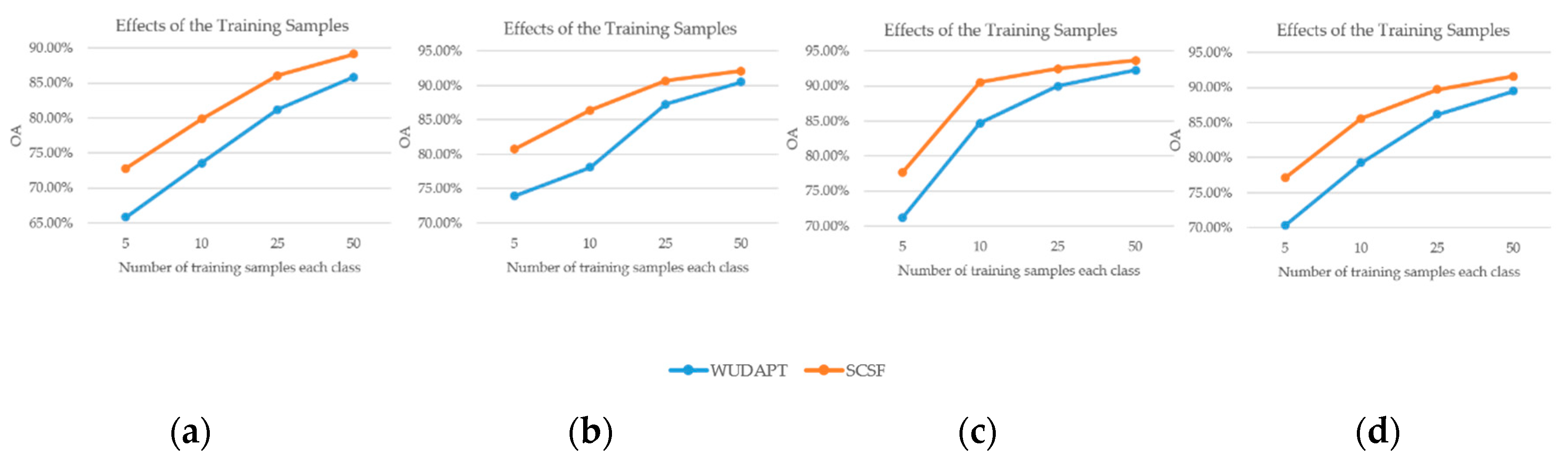
Table 3. This shows that the classification workflows considering spatial-contextual information (i.e., CI-WUDAPT, RF+MJ(WUDAPT), RF+CRF, RF+ST+MJ, and RF+ST+CRF(SCSF)) give a great improvement of nearly 5–18% in OA over the single classification results (i.e., NB, SVM, RF, and RF+ST) and an improvement of 0.06–0.2 in Kappa, proving the significance of the spatial-contextual information for LCZ mapping. Furthermore, the CRF-based classification workflows (i.e., RF+CRF and RF+ST+CRF(SCSF)) deliver an enhancement of approximately 4% in terms of OA and 0.05 in Kappa, compared with the independent majority-filter-based approaches (i.e., RF+MJ and RF+ST+MJ), which means that simultaneously modeling the correlation between labels and samples, in addition to the spatial relationship among samples, is very helpful. In addition, the accuracies of the self-training-based semi-supervised methods (i.e., RF+ST, RF+ST+MJ, and RF+ST+CRF(SCSF)) are higher than those of the supervised methods (i.e., RF, RF+MJ(WUDAPT), and RF+CRF), with improvements of nearly 2% and 0.2 in OA and Kappa, respectively, demonstrating the effectiveness of the generated pseudo-labels. The SVM classifier generates the worst accuracy with 18% lower than the SCSF in OA, which may be optimized through complex adjustment of its parameters. The CI-WUDAPT gives relatively high accuracy among the supervised methods; however, there is still a gap of 5% OA and 0.06 Kappa compared with the SCSF. The proposed RF+ST+CRF(SCSF) workflow shows the best quantitative performance among all the compared methods with only 10 labeled samples for each class, and the accuracies of 79.83% and 0.77 for OA and Kappa are also acceptable. However, the scattered LCZ types (i.e., LCZ 4 open high-rise, LCZ B scattered tree, and LCZ C bush or scrub) present inferior accuracies with semi-supervised methods, showing that the spatial-contextual information is insufficiently obtained from these LCZ types, which reduce the accuracies.

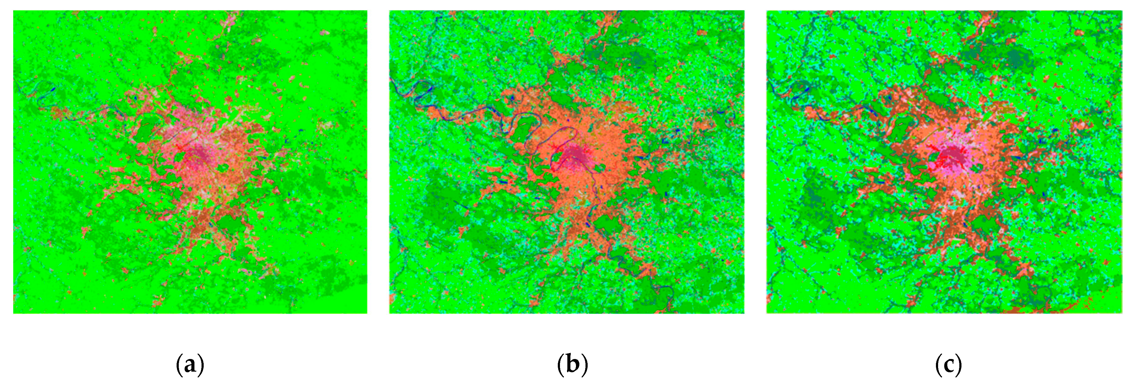
3.2.2. São Paulo Experiments

The second experimental area is São Paulo, Brazil, a city in the southern hemisphere with a more diverse urban form. The LCZ types in São Paulo cover almost all the built and natural classes except for LCZ 7 lightweight low-rise and LCZ C bush or scrub. Two cloudless Landsat-8 images from 2017DFC acquired on 8th February 2014 and 23rd September 2015 constituted the second experimental dataset. As in the first experiment, the images were down-sampled to a 100-m spatial resolution with a 1067 × 871 pixel dimension. Nine bands (i.e., bands 1–7 and 10–11) covering the infrared to visible spectrum were prepared. The RGB (i.e., bands 4, 3, 2) false-color image and the spatial distribution of the labeled data are shown in Figure 8a,b, respectively. Information about the class numbers is provided in Table 4.
The LCZ maps produced by the different approaches (i.e., NB, SVM, CI-WUDAPT, RF, RF+MJ(WUDAPT), RF+CRF, RF+ST, RF+ST+MJ, and RF+ST+CRF(SCSF)) are shown in Figure 9a–i. Differing from Berlin, much more salt-and-pepper noise appears in São Paulo with the RF-based classification (i.e., RF), which shows obvious changes after the majority-filter-based spatial smoothing (i.e., RF+MJ) and the CRF-based classification (i.e., RF+CRF). Although the prediction of RF+CRF presents much smoother class boundaries than the first two maps, the provided low-quality probabilistic map, which directly influences the modeling of the potential function, still brings a huge amount of misclassification. In particular, area 1 (green) of Figure 9f is supposed to be water, while the mislabeled spatial context confuses the CRF model, and the blue water region becomes green vegetation. Area 2 of Figure 9f is also heavily influenced by its surrounding mislabeled data, where LCZ 3 compact low-rise (rose red) is misclassified as LCZ 2 compact mid-rise (dark red). To relieve the above phenomena, the improved self-training-based classification (i.e., RF+ST, RF+ST+MJ, and RF+ST+CRF(SCSF)) was further adopted. Further improvements are apparent in Figure 9g–i with the improved self-training-based classification workflows (i.e., RF+ST, RF+ST+MJ, and RF+ST+CRF(SCSF)), and the appearance of scattered noise is much relieved when compared with the supervised results (i.e., RF, RF+MJ(WUDAPT), and RF+CRF). In particular, areas 1–2 of Figure 9i are accurately predicted to be real LCZ types, i.e., LCZ G water (blue) and LCZ 3 compact low-rise (rose red). The LCZ map generated by the proposed SCSF method provides not only an apparent visual improvement in better boundaries than the non-spatial-contextual information classification workflow (i.e., RF+ST) but also a cleaner and more accurate prediction than the result without self-training (i.e., RF+CRF). Moreover, the classifications of the NB, SVM, and CI-WUDAPT deliver quite different performances from that of SCSF. There are lots of misclassified noises that appear in Figure 9a,b and large misclassified areas stand out in Figure 9c, which prove that the visual performance of the SCSF is better than the previous researches.
Moreover, McNemar’s test between different methods (i.e., NB, SVM, CI-WUDAPT, RF, RF+MJ(WUDAPT), RF+CRF, RF+ST, RF+ST+MJ, and RF+ST+CRF(SCSF)) is shown in Table 5. All the values obtained among pairwise classification workflow are much greater than χ 0.05 , 1 2 ( 3.841459 ) , which means significant differences were found for the compared methods. The value of McNemar’s test between NB and SCSF is the biggest, indicating that the proposed workflow gives a significant statistical improvement compared with the classification of NB.
A quantitative report of the accuracies of the different methods (i.e., NB, SVM, CI-WUDAPT, RF, RF+MJ(WUDAPT), RF+CRF, RF+ST, RF+ST+MJ, and RF+ST+CRF(SCSF)) is given in Table 6. To evaluate the ability of the spatial-contextual information, the accuracies of RF and RF+ST serve as a baseline in the main part of the experiments and are compared with other workflows (i.e., RF+MJ(WUDAPT), RF+CRF, RF+ST+MJ, and RF+ST+CRF(SCSF)). The accuracies of the majority-filter-based spatial smoothing methods (i.e., RF+MJ(WUDAPT) and RF+ST+MJ) present an improvement of about 7% in OA and 0.07–0.08 in Kappa, while the CRF-based methods (i.e., RF+CRF and RF+ST+CRF(SCSF)) show a great improvement of nearly 12% in OA and 0.13–0.14 in Kappa. In addition, the generation of pseudo-labels from the self-training method provides an improvement of 3–4% in OA and 0.03–0.04 in Kappa for the supervised workflows (i.e., RF, RF+MJ(WUDAPT), and RF+CRF) and the corresponding semi-supervised approaches (i.e., RF+ST, RF+ST+MJ, and RF+ST+CRF(SCSF)), which demonstrates the effectiveness of the proposed strategy. Moreover, the NB classifier presents the worst performance with just 65.27% OA and 0.6 Kappa, which may prove that this kind of method is unsuitable for a city with diverse urban form in the case of limited samples. With the direct utilization of the spatial-contextual information, CI-WUDAPT shows 5-13% improvement in OA with the traditional approaches (i.e., NB, and SVM); however, the proposed SCSF method delivers a more superior performance in terms of OA and Kappa, with 86.4% and 0.84, respectively. Nevertheless, the LCZ types (i.e., LCZ 2 compact mid-rise, LCZ 4 open high-rise, LCZ 5 open mid-rise, LCZ B scattered trees, LCZ D low plants, LCZ E bare rock or paved, and LCZ F bare soil or sand) with relatively small testing samples present poor performance, which can be explained by the testing samples in São Paulo being clustered in the center areas and unable to reflect well the comprehensive condition.

3.2.3. Paris Experiments

The city of Paris in France was selected as the last experimental study area to assess the performance of the proposed SCSF method in a high-density city. The LCZ types are seven built types (i.e., LCZ 1 compact high-rise, LCZ 2 compact mid-rise, LCZ 4 open high-rise, LCZ 5 open mid-rise, LCZ 6 open low-rise, LCZ 8 large low-rise, and LCZ 9 sparsely built) and five natural types ( i.e., LCZ A dense trees, LCZ B scattered trees, LCZ D low plants, LCZ E bare rock or paved, and LCZ G water), revealing the multiformity of the urban region in Paris. The third experimental dataset comprised two Landsat 8 images of 1160 × 988 pixels provided by 2017DFC individually acquired on 19th May 2014 and 27th September 2015. The spatial resolution was again equal to 100 m after down-sampling, and the band information was the same as before, i.e., bands 1–7 and 10–11, amounting to nine channels. Figure 10a shows the false-color RGB image (i.e., bands 4,3,2), and an overview of the corresponding types is presented in Figure 10b. The sample numbers of each class are listed in Table 7.
The performance of the different methods (i.e., NB, SVM, CI-WUDAPT, RF, RF+MJ(WUDAPT), RF+CRF, RF+ST, RF+ST+MJ, and RF+ST+CRF(SCSF)) is shown in Figure 10a–i. The visual appearance of the salt-and-pepper noise in Paris seems more serious than for Berlin and São Paulo, while the variation of the categories is moderate. Compared with the results in the second column (i.e., RF and RF+ST), the other classification workflows (i.e., RF+MJ(WUDAPT), RF+CRF, RF+ST+MJ, and RF+ST+CRF(SCSF)) show an improvement in alleviating the noise issue with the further information from the spatial context. However, as in the São Paulo experiments, confusion appears in the results of RF+CRF, where the LCZ 4 open high-rise (rose red) in area 1 of Figure 11f is supposed to be LCZ 6 open low-rise (brown) and the LCZ C bush or scrub (light blue) in area 2 of Figure 11f is supposed to be LCZ A dense trees (green), which may have been caused by the insufficient training samples. The LCZ maps in the third row are the improved approaches (i.e., RF+ST, RF+ST+MJ, and RF+ST+CRF(SCSF)), and supported by the enrichment of the training data, the confused pixels decrease a lot from the beginning of the classification, compared with Figure 11d,f, which proves the significance of the training information. In particular, the misclassified areas 1–2 of Figure 11f are corrected to the real types, i.e., LCZ 6 open low-rise (brown) and LCZ A dense trees (green). The classifications of NB, SVM, and CI-WUDAPT in Paris are better than the above cities, which have less evident misclassified segments. However, the LCZ G water nearly disappears in Figure 11a and fragile noises or areas still stand out in Figure 11b,c. In addition, the developed SCSF workflow produces the best visual performance, with the elimination of the isolated pixels and the small, isolated areas.
Moreover, in order to give the statistical comparisons, McNemar’s values between the abovementioned methods (i.e., NB, SVM, CI-WUDAPT, RF, RF+MJ(WUDAPT), RF+CRF, RF+ST, RF+ST+MJ, and RF+ST+CRF(SCSF)) are given in Table 8. Similar to the other two cities, all the values of McNemar’s test in Paris are also greater than χ 0.05 , 1 2 ( 3.841459 ) , while the value between RF+CRF and SCSF (35.66) is relatively small compared with the RF and RF+CRF methods (1854.59) and the RF and SCSF methods (1854.51), showing that, although the semi-supervised approach gives some improvements in Paris, the spatial-contextual information-based CRF methods perform with more statistical significance.
In terms of the quantitative performance shown in Table 9, the experimental accuracies for Paris are much better than expected and reach the highest level among all three experiments. As in the previous experiments, the accuracies present different improvements with the assistance of the spatial context and the use of unlabeled data. To be specific, the result of the proposed SCSF method shows an improvement of about 7% in OA and 0.1 in Kappa compared with RF+ST; however, this is not apparent in the comparison with RF+ST+MJ and RF+CRF. The explanation for this is that, when the initial classification is already acceptable, the performance improvement of the proposed approach may not be that significant, since SCSF is aimed at solving the unreliable probability issue. Moreover, the accuracies of SCSF prevail over those of NB, SVM, and CI-WUDAPT, presenting about 6–16% and 0.08–0.2 improvement in OA and Kappa, respectively. In particular, LCZ types with an aggregation effect, such as LCZ D low plants, are obviously improved after fusing the spatial-contextual information. In contrast, the accuracies of some LCZ types which have dispersed spatial distribution and relatively small testing samples (i.e., LCZ 9 sparsely built, LCZ B scattered trees, and LCZ E bare rock or paved) present a decreased trend. Reasons can be explained as follows: (1) the SCSF is a spatial-contextual information-based method and, when the LCZ types are scattered or sparse, the spatial-contextual information is provided insufficiently, which may degrade the accuracies of these LCZ types; (2) the small number of testing samples for these LCZ types are unable to credibly evaluate the real condition.
In brief summary, for the main experimental part, the proposed SCSF gives the best performance in all three study areas compared with other five methods (i.e., RF, RF+MJ(WUDAPT), RF+CRF, RF+ST, and RF+ST+MJ) in terms of OA and Kappa, showing that the spatial-contextual information-based self-training classification framework for LCZs is undoubtedly effective. The values from McNemar’s test between the proposed SCSF with others are considerably large, which represents the significant differences from the statistical aspect. Moreover, the methods considering the spatial-contextual information (i.e., RF+MJ (WUDAPT), RF+CRF, RF+ST+MJ, and RF+ST+CRF(SCSF)) performed better than the other approaches (i.e., RF, and RF+ST), especially the CRF-based methods (i.e., RF+CRF, and RF+ST+CRF(SCSF)), which produce the best accuracies in OA and Kappa. Moreover, the semi-supervised approaches (i.e., RF+ST, RF+ST+MJ, and RF+ST+CRF(SCSF)) in the three experiments provide different improvements compared with the supervised methods (i.e., RF, RF+MJ, and RF+MJ (WUDAPT)).
Furthermore, the performances of the different methods (i.e., NB, SVM, and CI-WUDAPT) in three study areas are also considered to compare with the proposed SCSF, and the NB and SVM present relatively poor performances with many salt-and-pepper noises and misclassified areas. Moreover, the spatial-contextual information-based approaches (i.e., CI-WUDAPT, and SCSF) generate smoother predictions and SCSF delivers the best visual performance. Compared with the traditional machine learning classifier (i.e., NB and SVM), the proposed SCSF gives improvements of 10.65%–21.23% in OA with 0.13–0.24 in Kappa and 13.19%–18.58% in OA with 0.16–0.2 in Kappa, respectively. For CI-WUDAPT, the SCSF also outperforms it with 5.34%–7.75% in OA and 0.06–0.09 in Kappa, which proves the effectiveness of SCSF with the consideration of spatial-contextual information and self-training method.

4. Discussions

4.1. Effects of the Self-training Method

In order to test the effects of the improved self-training method, which applied the regional to local spatial-contextual information-based pseudo label selection as the strategy, different methods were used to make comparisons. To be specific, the proposed improved self-training method was compared with two other reference strategies. One benchmark was the original self-training approach, named ST-1, based on high-probability labels, which is usually unreliable, especially in the beginning. The other was the improved self-training method developed by Aydav and Minz, named ST-2 [44], based on the average probability in one granulation. The proposed self-training method based on regional and local information is denoted as STS. All of these methods were compared with the original RF classification results without the self-training step, which is denoted as RF. The OAs before and after the three different self-training approaches in the Berlin (BL), São Paulo (SP), and Paris (PA) datasets are listed in Table 10. The mean accuracy, denoted as mean, was also calculated to reflect the generic performance.
The quantitative report of the accuracies in Table 10 demonstrates that the ST-1 and ST-2 self-training approaches usually degrade the classification performance in both OA and Kappa, except for São Paulo (SP), where the accuracy of ST-2 is slightly increased. The explanation for this is that, since the initial classification accuracies (i.e., RF) are usually poor, the probability of predictions may be unreliable, while the strategy of ST-1 totally trusts high-probability pseudo-labels and ST-2 believes in the average probability among one granulation, resulting in misclassified noises which usually confuse the classifier. Given this fact, the proposed improved self-training method (i.e., STS) substitutes the spatial-contextual information from regional to local scales for the unreliable probability of the predictions, and the accuracy is enhanced by about 2–5% in OA and 0.02–0.07 in Kappa for the different cities. The generic results in the MEAN column also show the same trend, in that the proposed STS strategy presents the highest accuracies, which prove the effectiveness of the improved self-training method.
The LCZ maps conducted with the above approaches (i.e., RF, ST-1, ST-2, and STS) are shown in Figure 12a–l. Compared with the initial classification (i.e., RF), the LCZ maps based on ST-1 in the second column of Figure 12 generate lots of obvious misclassified noises over the whole image. Although the ST-2-based results represented by the third column although a lot compared with those of ST-1, noises still appear. Moreover, the classification results obtained using the STS strategy present more distinct class boundaries with less misclassified noises, which is evident in the visual performance. However, there are still many small, isolated areas appearing in the predictions, meaning that further consideration of the spatial-contextual information, i.e., the proposed CRF-based LCZ classification, is necessary.

4.2. Effects of the Sample Number

To analyze the effects of the initial sample number for the proposed SCSF, extra experiments were conducted in this section. Different sample numbers, i.e., 5, 10, 25, and 50 samples per class, were set to assess the proposed method, while the WUDAPT method was used as a reference. The generic results calculated by averaging the accuracies over all three areas are denoted as MEAN. Similar to the configuration of Section 3, the final experimental accuracies were the average performance of 10 run outcomes and the training samples were randomly selected in the whole ground truth data while the remaining was used as testing set.
As shown in Figure 13a–d, all the classifications exhibit a similar trend with the increase of the number for training samples. The experiments prove that the proposed SCSF has superior performance compared to WUDAPT in all the designed conditions. In terms of the performance in different areas, the biggest improvements between SCSF and WUDAPT are in Berlin, with 3–7% in OA. In more complex areas, i.e., São Paulo (SP) and Paris (PA), SCSF achieves a 1–7% improvement of OA. For the generic comparisons shown in the last column of Table 11 and Figure 13, the SCSF also presents a good performance. However, the accuracies of the LCZ maps with relatively large improvement using the SCSF have actually lower values than others, which means the proposed SCSF is more suitable to enhance the accuracy when the initial classification is really poor.
Furthermore, the proposed SCSF shows a strong performance, especially with a small number of training samples, but the OA shows a higher growth with 5/10 samples compared to 25/50 samples per class; for instance, when the accuracy with 25 or 50 samples in Paris (PA) is already over 90%, the improvement is only about 1–2%. Moreover, the proposed SCSF method is capable of generating an equivalent accuracy to the WUDAPT method with fewer training samples. In particular, the OA with five samples in São Paulo (SP) shows a similar performance to the WUDAPT method using 10 samples per class. In terms of OA, the SCSF method shows great improvement with different sample numbers (i.e., 5, 10, 25, and 50 samples per class) compared with WUDAPT, which shows that the SCSF is really helpful for LCZ classification.

5. Conclusions

In this paper, we have proposed a spatial-contextual information-based self-training classification framework (SCSF) for LCZs, which introduces CRF for LCZ classification to better utilize the spatial-contextual information and probabilistic classification with self-training to provide more reliable inputs for CRF. Three experiments using Landsat 8 images from three diverse areas—Berlin, São Paulo, and Paris—confirmed the effectiveness of the proposed SCSF method with the widely used protocol developed by WUDAPT.
To be specific, the CRF provides a unified theoretical foundation for directly bringing the spatial-contextual information into classification, mitigating both the appearance of salt-and-pepper noise and small, isolated noise areas. In addition, probabilistic classification provided with an improved self-training-based approach is adopted to consider the lack of high-quality expert-labeled data. Through the enrichment of the limited training data with pseudo-labels, the predicted probability used for the potential function modeling is more reliable.
Moreover, the effects of the improved self-training method and the sensitivity to different sample numbers were also investigated. Overall, the proposed SCSF method showed powerful quantitative and qualitative performances in LCZ mapping not only in the multiform city but also in the high-density city, especially when the training data were limited. In our future work, we will explore the use of a deep learning method for LCZ classification, and other data and larger study areas will also be considered.

Author Contributions

Conceptualization, N.Z., A.M., and Y.Z.; data curation, N.Z.; funding acquisition, A.M. and Y.Z.; methodology, N.Z., A.M., Y.Z., and J.Z.; supervision, A.M. and Y.Z.; validation, N.Z.; writing—original draft, N.Z. and Y.Z.; writing—review and editing, N.Z., A.M., Y.Z., J.Z., and L.C.

Funding

This work was supported by National Key Research and Development Program of China under Grant No. 2017YFB0504202, National Natural Science Foundation of China under Grant Nos. 41622107, 41771385, 41801267, in part by the China Postdoctoral Science Foundation under Grant 2017M622522, in part by the Fundamental Research Funds for the Central Universities under grant no. 2042018kf0229.

Acknowledgments

The authors are particularly grateful to the 2017 Data Fusion Contest for providing the datasets.

Conflicts of Interest

The authors declare no conflict of interest.

References

  1. Stewart, I.D.; Oke, T.R. Local Climate Zones for Urban Temperature Studies. Bull. Am. Meteorol. Soc. 2012, 93, 1879–1900. [Google Scholar] [CrossRef]
  2. Bechtel, B.; Conrad, O.; Tamminga, M.; Verdonck, M.-L.; Van Coillie, F.; Tuia, D.; Demuzere, M.; See, L.; Lopes, P.; Fonte, C.C. Beyond the urban mask. In Proceedings of the 2017 Joint Urban Remote Sensing Event (JURSE), Dubai, UAE, 6–8 March 2017; pp. 1–4. [Google Scholar]
  3. Wang, C.; Middel, A.; Myint, S.W.; Kaplan, S.; Brazel, A.J.; Lukasczyk, J. Assessing local climate zones in arid cities: The case of Phoenix, Arizona and Las Vegas, Nevada. ISPRS J. Photogramm. Remote Sens. 2018, 141, 59–71. [Google Scholar] [CrossRef]
  4. Quan, J. Multi-Temporal Effects of Urban Forms and Functions on Urban Heat Islands Based on Local Climate Zone Classification. Int. J. Environ. Res. Public Health 2019, 16, 2140. [Google Scholar] [CrossRef] [PubMed]
  5. Perera, N.; Emmanuel, R. A “Local Climate Zone” based approach to urban planning in Colombo, Sri Lanka. Urban Clim. 2018, 23, 188–203. [Google Scholar] [CrossRef]
  6. Ren, C.; Cai, M.; Wang, R.; Xu, Y.; Ng, E. Local climate zone (LCZ) classification using the world urban database and access portal tools (WUDAPT) method: A case study in Wuhan and Hangzhou. In Proceedings of the Countermeasure Urban Heat Islands, Singapore, May 30–June 1 2016. [Google Scholar]
  7. Brousse, O.; Martilli, A.; Foley, M.; Mills, G.; Bechtel, B. WUDAPT, an efficient land use producing data tool for mesoscale models? Integration of urban LCZ in WRF over Madrid. Urban Clim. 2016, 17, 116–134. [Google Scholar] [CrossRef]
  8. Brousse, O.; Georganos, S.; Demuzere, M.; Vanhuysse, S.; Wouters, H.; Wolff, E.; Linard, C.; Nicole, P.-M.; Dujardin, S. using local climate zones in Sub-Saharan Africa to tackle urban health issues. Urban Clim. 2019, 27, 227–242. [Google Scholar] [CrossRef]
  9. Alexander, P.J.; Mills, G.; Fealy, R. Using LCZ data to run an urban energy balance model. Urban Clim. 2015, 13, 14–37. [Google Scholar] [CrossRef]
  10. Wang, R.; Ren, C.; Xu, Y.; Lau, K.K.-L.; Shi, Y. Mapping the local climate zones of urban areas by GIS-based and WUDAPT methods: A case study of Hong Kong. Urban Clim. 2018, 24, 567–576. [Google Scholar] [CrossRef]
  11. Zheng, Y.; Ren, C.; Xu, Y.; Wang, R.; Ho, J.; Lau, K.; Ng, E. GIS-based mapping of Local Climate Zone in the high-density city of Hong Kong. Urban Clim. 2018, 24, 419–448. [Google Scholar] [CrossRef]
  12. Gál, T.; Bechtel, B.; Unger, J. Comparison of Two Different Local Climate Zone Mapping Methods. In Proceedings of the 9th International Conference on Urban Climate Jointly with 12th Symposium on the Urban Environment, Toulouse, France, 20–24 July 2015. [Google Scholar]
  13. Lelovics, E.; Unger, J.; Gál, T.; Gál, C.V. Design of an urban monitoring network based on Local Climate Zone mapping and temperature pattern modelling. Clim. Res. 2014, 60, 51–62. [Google Scholar] [CrossRef]
  14. Geletič, J.; Lehnert, M. GIS-based delineation of local climate zones: The case of medium-sized Central European cities. Morav. Geogr. Rep. 2016, 24, 2–12. [Google Scholar] [CrossRef]
  15. See, L.; Perger, C.; Duerauer, M.; Fritz, S.; Bechtel, B.; Ching, J.; Alexander, P.; Mills, G.; Foley, M.; O’Connor, M. Developing a community-based worldwide urban morphology and materials database (WUDAPT) using remote sensing and crowdsourcing for improved urban climate modelling. In Proceedings of the 2015 Joint Urban Remote Sensing Event (JURSE), Lausanne, Switzerland, 30 March–1 April 2015; pp. 1–4. [Google Scholar]
  16. Ching, J.; See, L.; Mills, G.; Alexander, P.; Bechtel, B.; Feddema, J.; Oleson, K.L.; Stewart, I.; Neophytou, M.; Chen, F. WUDAPT: Facilitating advanced urban canopy modeling for weather, climate and air quality applications. In Proceedings of the 94th American Meterological Society Annual Meeting, Atlanta, GA, USA, 2–6 February 2014. [Google Scholar]
  17. Xu, Z.; Chen, J.; Xia, J.; Du, P.; Zheng, H.; Gan, L. Multisource earth observation data for land-cover classification using random forest. IEEE Geosci. Remote Sens. Lett. 2018, 15, 789–793. [Google Scholar] [CrossRef]
  18. Conrad, O.; Bechtel, B.; Bock, M.; Dietrich, H.; Fischer, E.; Gerlitz, L.; Wehberg, J.; Wichmann, V.; Böhner, J. System for automated geoscientific analyses (SAGA) v.2.1.4. Geosci. Model Dev. 2015, 8, 1991–2007. [Google Scholar] [CrossRef]
  19. Bechtel, B.; Alexander, P.; Böhner, J.; Ching, J.; Conrad, O.; Feddema, J.; Mills, G.; See, L.; Stewart, I. Mapping local climate zones for a worldwide database of the form and function of cities. ISPRS Int. J. Geo Inf. 2015, 4, 199–219. [Google Scholar] [CrossRef]
  20. Demuzere, M.; Bechtel, B.; Middel, A.; Mills, G. Mapping Europe into local climate zones. PLoS ONE 2019, 14, e0214474. [Google Scholar] [CrossRef] [PubMed]
  21. Bechtel, B.; Demuzere, M.; Mills, G.; Zhan, W.; Sismanidis, P.; Small, C.; Voogt, J. SUHI analysis using Local Climate Zones—A comparison of 50 cities. Urban Clim. 2019, 28, 100451. [Google Scholar] [CrossRef]
  22. Shi, Y.; Ren, C.; Lau, K.K.-L.; Ng, E. Investigating the influence of urban land use and landscape pattern on PM2.5 spatial variation using mobile monitoring and WUDAPT. Landsc. Urban Plan. 2019, 189, 15–26. [Google Scholar] [CrossRef]
  23. Collins, J.; Dronova, I. Urban Landscape Change Analysis Using Local Climate Zones and Object-Based Classification in the Salt Lake Metro Region, Utah, USA. Remote Sens. 2019, 11, 1615. [Google Scholar] [CrossRef]
  24. Liu, S.; Qi, Z.; Li, X.; Yeh, A.G.-O. Integration of Convolutional Neural Networks and Object-Based Post-Classification Refinement for Land Use and Land Cover Mapping with Optical and SAR Data. Remote Sens. 2019, 11, 690. [Google Scholar] [CrossRef]
  25. Sukhanov, S.; Tankoyeu, I.; Louradour, J.; Heremans, R.; Trofimova, D.; Debes, C. Multilevel ensembling for local climate zones classification. In Proceedings of the 2017 IEEE International Geoscience and Remote Sensing Symposium (IGARSS), Fort Worth, TX, USA, 23–28 July 2017; pp. 1201–1204. [Google Scholar]
  26. Qiu, C.; Schmitt, M.; Mou, L.; Ghamisi, P.; Zhu, X. Feature importance analysis for local climate zone classification using a residual convolutional neural network with multi-source datasets. Remote Sens. 2018, 10, 1572. [Google Scholar] [CrossRef]
  27. Qiu, C.; Mou, L.; Schmitt, M.; Zhu, X.X. Local climate zone-based urban land cover classification from multi-seasonal Sentinel-2 images with a recurrent residual network. ISPRS J. Photogramm. Remote Sens. 2019, 154, 151–162. [Google Scholar] [CrossRef] [PubMed]
  28. Yoo, C.; Han, D.; Im, J.; Bechtel, B. Comparison between convolutional neural networks and random forest for local climate zone classification in mega urban areas using Landsat images. ISPRS J. Photogramm. Remote Sens. 2019, 157, 155–170. [Google Scholar] [CrossRef]
  29. Panboonyuen, T.; Jitkajornwanich, K.; Lawawirojwong, S.; Srestasathiern, P.; Vateekul, P. Road Segmentation of Remotely-Sensed Images Using Deep Convolutional Neural Networks with Landscape Metrics and Conditional Random Fields. Remote Sens. 2017, 9, 680. [Google Scholar] [CrossRef]
  30. Ma, F.; Gao, F.; Sun, J.; Zhou, H.; Hussain, A. Weakly Supervised Segmentation of SAR Imagery Using Superpixel and Hierarchically Adversarial CRF. Remote Sens. 2019, 11, 512. [Google Scholar] [CrossRef]
  31. Zhang, B.; Wang, C.; Shen, Y.; Liu, Y. Fully Connected Conditional Random Fields for High-Resolution Remote Sensing Land Use/Land Cover Classification with Convolutional Neural Networks. Remote Sens. 2018, 10, 1889. [Google Scholar] [CrossRef]
  32. Wei, L.; Yu, M.; Liang, Y.; Yuan, Z.; Huang, C.; Li, R.; Yu, Y. Precise Crop Classification Using Spectral-Spatial-Location Fusion Based on Conditional Random Fields for UAV-Borne Hyperspectral Remote Sensing Imagery. Remote Sens. 2019, 11, 2011. [Google Scholar] [CrossRef]
  33. Wei, L.; Yu, M.; Zhong, Y.; Zhao, J.; Liang, Y.; Hu, X. Spatial–Spectral Fusion Based on Conditional Random Fields for the Fine Classification of Crops in UAV-Borne Hyperspectral Remote Sensing Imagery. Remote Sens. 2019, 11, 780. [Google Scholar] [CrossRef]
  34. Zhong, Y.; Cao, Q.; Zhao, J.; Ma, A.; Zhao, B.; Zhang, L. Optimal Decision Fusion for Urban Land-Use/Land-Cover Classification Based on Adaptive Differential Evolution Using Hyperspectral and LiDAR Data. Remote Sens. 2017, 9, 868. [Google Scholar] [CrossRef]
  35. Wang, J. The Urban Land Surface Thermal Environment Dynamics and Optimization Recommendations. Ph.D. Thesis, Wuhan University, Wuhan, China, 2016. [Google Scholar]
  36. Mills, G.; Ching, J.; See, L.; Bechtel, B.; Foley, M. An Introduction to the WUDAPT project. In Proceedings of the 9th International Conference on Urban Climate, Toulouse, France, 20–24 July 2015. [Google Scholar]
  37. See, L.; Mills, G.; Ching, J. Community initiative tackles urban heat. Nature 2015, 526, 43. [Google Scholar] [CrossRef]
  38. Scudder, H. Probability of error of some adaptive pattern-recognition machines. IEEE Trans. Inf. Theory 1965, 11, 363–371. [Google Scholar] [CrossRef]
  39. Subramanya, A.; Petrov, S.; Pereira, F. Efficient graph-based semi-supervised learning of structured tagging models. In Proceedings of the 2010 Conference on Empirical Methods in Natural Language Processing, Cambridge, MA, USA, 9–10 October 2010; pp. 167–176. [Google Scholar]
  40. Besemer, J.; Lomsadze, A.; Borodovsky, M. GeneMarkS: A self-training method for prediction of gene starts in microbial genomes. Implications for finding sequence motifs in regulatory regions. Nucleic Acids Res. 2001, 29, 2607–2618. [Google Scholar] [CrossRef] [PubMed] [Green Version]
  41. McClosky, D.; Charniak, E.; Johnson, M. Effective self-training for parsing. In Proceedings of the Main Conference on Human Language Technology Conference of the North American Chapter of the Association of Computational Linguistics, New York, NY, USA, 4–9 June 2006; pp. 152–159. [Google Scholar]
  42. Kim, Y.; Park, N.-W.; Lee, K.-D. Self-Learning Based Land-Cover Classification Using Sequential Class Patterns from Past Land-Cover Maps. Remote Sens. 2017, 9, 921. [Google Scholar] [CrossRef] [Green Version]
  43. Li, Y.; Xing, R.; Jiao, L.; Chen, Y.; Chai, Y.; Marturi, N.; Shang, R. Semi-Supervised PolSAR Image Classification Based on Self-Training and Superpixels. Remote Sens. 2019, 11, 1933. [Google Scholar] [CrossRef] [Green Version]
  44. Aydav, P.S.S.; Minz, S. Granulation-Based Self-Training for the Semi-Supervised Classification of Remote-Sensing Images. Granular Computing; Springer: Berlin/Heidelberg, Germany, 2019; pp. 1–19. [Google Scholar]
  45. Verdonck, M.-L.; Okujeni, A.; van der Linden, S.; Demuzere, M.; De Wulf, R.; Van Coillie, F. Influence of neighbourhood information on ‘Local Climate Zone’mapping in heterogeneous cities. Int. J. Appl. Earth Obs. Geoinf. 2017, 62, 102–113. [Google Scholar] [CrossRef]
  46. Han-Qiu, X. A study on information extraction of water body with the modified normalized difference water index (MNDWI). J. Remote Sens. 2005, 5, 589–595. [Google Scholar]
  47. Rouse, J.W., Jr.; Haas, R.; Schell, J.; Deering, D. Monitoring Vegetation Systems in the Great Plains with ERTS; NASA: Washington, DC, USA, 1974.
  48. Jordan, C.F. Derivation of leaf-area index from quality of light on the forest floor. Ecology 1969, 50, 663–666. [Google Scholar] [CrossRef]
  49. Jamalabad, M. Forest canopy density monitoring using satellite images. In Proceedings of the Geo-Imagery Bridging Continents XXth ISPRS Congress, Istanbul, Turkey, 12–23 July 2004. [Google Scholar]
  50. Zha, Y.; Gao, J.; Ni, S. Use of normalized difference built-up index in automatically mapping urban areas from TM imagery. Int. J. Remote Sens. 2003, 24, 583–594. [Google Scholar] [CrossRef]
  51. Xu, H. Analysis of impervious surface and its impact on urban heat environment using the normalized difference impervious surface index (NDISI). Photogramm. Eng. Remote. Sens. 2010, 76, 557–565. [Google Scholar] [CrossRef]
  52. Felzenszwalb, P.F.; Huttenlocher, D.P. Efficient graph-based image segmentation. Int. J. Comput. Vis. 2004, 59, 167–181. [Google Scholar] [CrossRef]
  53. Breiman, L. Random forests. Mach. Learn. 2001, 45, 5–32. [Google Scholar] [CrossRef] [Green Version]
  54. Li, B.; Friedman, J.; Olshen, R.A.; Stone, C.J. Classification and Regression Trees (CART); Chapman and Hall/CRC: Abingdon, UK, 1984; Volume 40, p. 358. [Google Scholar]
  55. Zhang, G.; Jia, X. Simplified conditional random fields with class boundary constraint for spectral-spatial based remote sensing image classification. IEEE Geosci. Remote Sens. Lett. 2012, 9, 856–860. [Google Scholar] [CrossRef]
  56. Zhong, Y.; Zhao, J.; Zhang, L. A hybrid object-oriented conditional random field classification framework for high spatial resolution remote sensing imagery. IEEE Trans. Geosci. Remote Sens. 2014, 52, 7023–7037. [Google Scholar] [CrossRef]
  57. Bechtel, B.; Daneke, C. Classification of local climate zones based on multiple earth observation data. IEEE J. Sel. Top. Appl. Earth Obs. Remote Sens. 2012, 5, 1191–1202. [Google Scholar] [CrossRef]
  58. Bechtel, B.; See, L.; Mills, G.; Foley, M. Classification of local climate zones using SAR and multispectral data in an arid environment. IEEE J. Sel. Top. Appl. Earth Obs. Remote Sens. 2016, 9, 3097–3105. [Google Scholar] [CrossRef]
  59. Qiua, C.P.; Schmitta, M.; Ghamisib, P.; Zhua, X.X. Effect of the Training Set Configuration on Sentinel-2-Based under Local Climate Zone Classification. Int. Arch. Photogramm. Remote Sens. Spat. Inf. Sci. 2018, 42, 931–936. [Google Scholar] [CrossRef] [Green Version]
  60. Lu, X.; Zhang, J.; Li, T.; Zhang, Y. Hyperspectral Image Classification Based on Semi-Supervised Rotation Forest. Remote Sens. 2017, 9, 924. [Google Scholar]
  61. Fazakis, N.; Kanas, V.G.; Aridas, C.K.; Karlos, S.; Kotsiantis, S. Combination of Active Learning and Semi-Supervised Learning under a Self-Training Scheme. Entropy 2019, 21, 988. [Google Scholar] [CrossRef] [Green Version]
  62. McNemar, Q. Note on the sampling error of the difference between correlated proportions or percentages. Psychometrika 1947, 12, 153–157. [Google Scholar] [CrossRef]
Figure 1. The local climate zone scheme.
Remotesensing 11 02828 g001
Figure 2. The workflow of the Local Climate Zone (LCZ) mapping approach proposed by the World Urban Database and Access Portal Tool (WUDAPT) project. ROI-Region of interest; KML-Keyhole markup language; ViGrA- An image processing library.
Remotesensing 11 02828 g002
Figure 3. The framework of the self-training algorithm.
Remotesensing 11 02828 g003
Figure 4. The framework of the proposed methodology (spatial-contextual information-based self-training classification framework (SCSF)).
Remotesensing 11 02828 g004
Figure 5. The improved self-training method.
Remotesensing 11 02828 g005
Figure 6. Berlin Landsat 8 dataset. (a) RGB false-color image (4, 3, 2). (b) Ground-truth image.
Remotesensing 11 02828 g006
Figure 7. The classification maps for the Berlin Landsat 8 data: (a) Naive Bayes (NB), (b) Support Vector Machine (SVM), (c) the improved WUDAPT method (CI-WUDAPT), (d) random forest (RF), (e) WUDAPT, (f) RF+conditional random fields (CRF), (g) RF+self-training method (ST), (h) RF+ST+majority filter(MJ), and (i) SCSF.
Remotesensing 11 02828 g007aRemotesensing 11 02828 g007b
Figure 8. São Paulo Landsat 8 dataset: (a) RGB false-color image (4, 3, 2). (b) Ground-truth image.
Remotesensing 11 02828 g008
Figure 9. The classification maps for the São Paulo Landsat 8 data: (a) NB, (b) SVM, (c) CI-WUDAPT, (d) RF, (e) WUDAPT, (f) RF+CRF, (g) RF+ST, (h) RF+ST+MJ, and (i) SCSF.
Remotesensing 11 02828 g009
Figure 10. Paris Landsat 8 dataset: (a) RGB false-color image (4, 3, 2). (b) Ground-truth image.
Remotesensing 11 02828 g010
Figure 11. The classification maps for the Paris Landsat 8 data: (a) NB, (b) SVM, (c) CI-WUDAPT, (d) RF, (e) WUDAPT, (f) RF+CRF, (g) RF+ST, (h) RF+ST+MJ, and (i) SCSF.
Remotesensing 11 02828 g011aRemotesensing 11 02828 g011b
Figure 12. Classification results for different methods. Berlin: (a) RF, (b) ST-1, (c) ST-2, and (d) STS; São Paulo: (e) RF, (f) ST-1, (g) ST-2, and (h) STS; and Paris: (i) RF, (j) ST-1, (k) ST-2, and (l) STS.
Remotesensing 11 02828 g012aRemotesensing 11 02828 g012b
Figure 13. The OA of different sample numbers, with three study areas and the average performance: (a) Berlin, (b) São Paulo, (c) Paris, and (d) MEAN.
Remotesensing 11 02828 g013
Table 1. Class information for Berlin.
LCZ Class245689ABCDFG
Samples153457724484010165476149601028105044243591732
Table 2. McNemar’s test for the Berlin Landsat 8 data.
SCSFRF+ST+MJRF+STRF+CRFWUDAPTRFCI-WUDAPTSVMNB
SCSFNA502.121533.52309.06700.331750.63449.522970.461610.06
RF+ ST+MJ NA653.09213.40144.18802.29105.691907.11733.18
RF+ST NA847.38248.97115.85327.02788.59163.26
RF+CRF NA404.541438.25224.402434.481220.01
WUDAPT NA691.5479.911488.81495.67
RF NA528.75466.36116.25
CI-WUDAPT NA1780.09494.02
SVM NA482.81
NB NA
Table 3. Accuracies of the different methods for the Berlin data.
AccuracySupervisedSemi-Supervised
NBSVMCI-WUDAPTRFWUDAPTRF+CRFRF+STRF+ST+MJSCSF
LCZ 270.90%87.90%86.40%81.90%92.60%89.90%83.00%94.80%92.70%
LCZ 462.70%33.80%78.40%57.70%78.40%82.10%54.50%74.50%76.50%
LCZ 536.90%40.30%57.20%36.20%39.20%48.00%37.90%41.80%50.50%
LCZ 657.20%66.60%68.40%65.60%74.90%77.20%63.40%72.60%77.60%
LCZ 850.70%18.90%74.20%43.80%52.90%59.10%41.90%51.40%62.60%
LCZ 954.20%51.80%58.50%62.90%74.10%76.70%65.20%73.30%73.70%
LCZ A81.90%71.20%87.00%83.20%86.10%86.30%88.30%90.40%92.20%
LCZ B60.10%46.40%65.80%68.10%75.90%82.10%66.00%74.90%81.40%
LCZ C51.10%28.30%54.30%50.50%55.70%65.80%43.90%47.30%53.30%
LCZ D83.20%64.30%73.30%65.70%70.30%78.40%75.30%78.60%84.90%
LCZ F75.10%65.60%73.60%79.10%83.70%88.90%79.20%83.60%87.00%
LCZ G91.00%100.00%92.50%100.00%100.00%100.00%100.00%100.00%100.00%
OA67.85%61.25%74.49%67.57%73.54%77.52%69.70%75.35%79.83%
Kappa0.640.570.710.640.700.750.660.720.77
Table 4. Class information for São Paulo.
LCZ Class1234568910ABDEFG
Samples95513453084822441862191533517963593023761091443492
Table 5. McNemar’s test for the São Paulo Landsat 8 data.
SCSFRF+ST+MJRF+STRF+CRFWUDAPTRFCI-WUDAPTSVMNB
SCSFNA484.381888.02389.101063.392381.711056.862062.363635.94
RF+ST+MJ NA934.36261.99367.001244.79386.981092.812364.92
RF+ST NA1076.55213.15151.35309.99194.60962.25
RF+CRF NA606.681759.44543.281271.602889.08
WUDAPT NA487.5577.45339.691492.06
RF NA553.46144.91572.27
CI-WUDAPT NA354.671548.63
SVM NA629.39
NB NA
Table 6. Accuracies of the different methods for the São Paulo data.
AccuracySupervisedSemi-Supervised
NBSVMCI-WUDAPTRFWUDAPTRF+CRFRF+STRF+ST+MJSCSF
LCZ 154.70%70.40%72.90%68.30%75.80%85.00%70.50%88.50%88.80%
LCZ 237.30%13.80%40.90%36.30%28.40%60.50%32.70%48.00%48.70%
LCZ 358.00%77.30%81.10%59.90%87.00%75.30%66.70%78.80%81.40%
LCZ 443.20%31.50%48.80%35.20%41.70%51.90%34.70%42.80%49.40%
LCZ 534.40%23.30%40.70%35.40%30.80%58.40%31.40%43.80%60.00%
LCZ 644.20%26.70%44.80%40.90%42.40%65.20%44.30%59.20%72.40%
LCZ 849.20%26.60%75.00%40.00%52.70%68.40%40.40%52.50%73.50%
LCZ 948.00%40.40%65.20%58.50%63.10%82.20%56.20%77.40%81.40%
LCZ 1043.10%8.30%39.90%39.20%12.10%81.10%41.00%60.00%78.60%
LCZ A79.00%98.10%91.50%96.10%93.90%98.30%98.80%99.90%99.30%
LCZ B50.60%31.10%55.30%46.30%48.10%67.40%41.30%46.70%60.70%
LCZ D58.00%44.00%50.70%41.50%42.10%63.10%44.60%49.60%62.00%
LCZ E43.40%5.80%28.80%38.90%9.70%54.30%37.80%46.60%57.40%
LCZ F66.30%57.40%68.90%61.80%60.30%71.70%61.60%68.30%66.40%
LCZ G85.30%99.00%91.10%98.60%93.00%99.30%99.00%99.70%99.20%
OA65.27%73.21%78.65%71.78%78.11%83.64%74.62%81.96%86.40%
Kappa0.600.680.750.67 0.740.80 0.70 0.78 0.84
Table 7. Class information for Paris.
LCZ Class1245689ABDEG
Samples56270536644624197486044973947688214234
Table 8. McNemar’s test for the Paris Landsat 8 data.
SCSFRF+ST+MJRF+STRF+CRFWUDAPTRFCI-WUDAPTSVMNB
SCSFNA107.12906.8835.66617.951854.51597.032519.431433.92
RF+ST+MJ NA787.4557.15415.521640.60424.962277.861184.57
RF+ST NA678.61101.75489.50133.66947.55464.72
RF+CRF NA590.181854.59493.442351.131297.77
WUDAPT NA944.55245.381247.83638.13
RF NA641.06215.03434.37
CI-WUDAPT NA1218.63358.97
SVM NA477.69
NB NA
Table 9. Accuracies of the different methods for the Paris data.
AccuracySupervisedSemi-Supervised
NBSVMCI-WUDAPTRFWUDAPTRF+CRFRF+STRF+ST+MJSCSF
LCZ 168.00%64.50%88.30%69.10%91.50%86.00%63.50%91.20%89.90%
LCZ 265.70%79.50%86.10%77.20%89.20%89.90%78.30%90.40%90.30%
LCZ 444.50%40.00%53.40%41.60%51.90%55.50%40.20%51.70%57.20%
LCZ 540.70%49.30%58.80%47.70%60.40%64.20%42.30%54.40%62.20%
LCZ 661.70%60.10%61.90%69.50%76.30%71.80%72.20%79.60%74.40%
LCZ 865.00%73.70%80.40%72.50%85.60%89.70%67.40%83.10%87.20%
LCZ 963.40%68.60%87.40%72.20%88.80%90.80%59.80%73.60%46.00%
LCZ A78.50%91.80%88.70%90.70%94.70%96.30%92.70%96.30%97.50%
LCZ B68.50%72.90%87.10%74.00%77.10%76.70%63.00%64.90%61.40%
LCZ D98.00%69.40%92.80%76.10%83.40%96.10%90.60%94.10%97.40%
LCZ E55.30%47.40%57.10%54.60%59.60%60.00%56.60%61.20%53.80%
LCZ G83.10%93.90%91.90%92.70%96.00%95.30%92.30%95.60%95.60%
OA79.89%73.99%84.73%77.27%84.72%89.87%83.31%89.30%90.54%
Kappa0.740.680.800.720.810.870.780.860.88
Table 10. Accuracies in different areas (%).
MethodBLSPPAMEAN
OAKappaOAKappaOAKappaOAKappa
RF67.57%0.6471.78%0.6777.27%0.7272.21%0.67
ST-165.16%0.6170.66%0.6573.08%0.6769.64%0.64
ST-266.23%0.6273.45%0.6876.48%0.7172.05%0.67
STS69.70%0.6674.62%0.7083.31%0.7875.88%0.71
Notes: BL-Accuracies in Berlin; SP-Accuracies in São Paulo; PA-Accuracies in Paris; MEAN-Average accuracies in the whole three cities.
Table 11. The OA with different sample numbers (%).
SamplesBLSPPAMEAN
WUDAPTSCSFWUDAPTSCSFWUDAPTSCSFWUDAPTSCSF
565.83%72.81%73.91%80.75%71.21%77.71%70.32%77.09%
1073.54%79.83%78.11%86.40%84.72%90.54%79.27%85.59%
2581.22%86.05%87.29%90.65%90.02%92.50%86.18%89.73%
5085.82%89.15%90.52%92.12%92.24%93.65%89.53%91.64%

