Optimal Assimilation of Daytime SST Retrievals from SEVIRI in a Regional Ocean Prediction System

Abstract

Exploiting the potential of space-borne oceanic measurements to characterize the sub-surface structure of the ocean becomes critical in areas where deployment of in situ sensors might be difficult or expensive. Sea Surface Temperature (SST) observations potentially provide enormous amounts of information about the upper ocean variability. However, the assimilation of daytime SST retrievals, e.g., from infrared sensors into ocean prediction systems, requires a specific treatment of the diurnal cycle of skin SST, which is generally under-estimated in current ocean models due to poor vertical resolution at the air–sea interface and lack of proper parameterizations. To this end, a simple off-line bias correction scheme is proposed, where the bias predictors include, among others, the warm layer and cool skin warming/cooling deduced from a prognostic model. Furthermore, a localization procedure that limits the vertical penetration of the SST information in a hybrid variational-ensemble data assimilation system is formulated. These two novelties are implemented and assessed within a regional ocean prediction system in the Ligurian Sea for the assimilation of daytime SST data retrieved with hourly frequency from the Spinning Enhanced Visible and Infrared Imager (SEVIRI) onboard the geostationary satellite Meteosat-10. Experiments are validated against independent measurements collected by gliders, moorings, and drifters during the Long-term Glider Missions for Environmental Characterization (LOGCMEC17) sea trial. Results suggest that the simple bias correction scheme is effective in improving both the sea surface and mixed layer accuracy, correctly thinning the mixed layer compared to the control experiment, outperforming experiments with night-only data assimilation, and improving the forecast skill scores. Localization further improves the prediction of the mixed layer depth. It is therefore recommended that sophisticated bias correction and localization procedures are adopted for fruitfully assimilating daytime SST data in operational oceanographic analysis systems.

1. Introduction

Within regional ocean prediction systems and high-resolution environmental characterizations, the optimal exploitation of remotely sensed data becomes increasingly important [1,2], due to the high costs that deployment and maintenance of high-resolution in situ measurements require [3]. Thus, techniques aiming at improving the way sea surface observations from satellite-borne sensors correct the sub-surface ocean state are required to advance. Here, we focus our investigation on the optimal assimilation of daytime sea surface temperature (SST) retrievals at high temporal frequency, which has the potential to correct the mixed layer depth [4,5,6], with obvious advantages for several oceanographic applications, ranging from biogeochemistry to underwater acoustic propagation [7].

Although SST measurements from infrared sensors onboard polar-orbiting satellites have been available for a long time, little use of daytime data has been made in operational contexts due to the difficulty of modeling the surface layer diurnal variability in Ocean General Circulation Models (OGCMs). This has induced most prediction systems to assimilate only nighttime SST measurements, thus avoiding the use of data potentially affected by diurnal warming and biases [8]. Over the last decade, the vertical resolution of OGCMs has significantly increased; consequently, the top model levels have risen and have become much shallower than before. In particular, the first vertical level is generally included within the first meter of the water column or less, even in global OGCMs [9]. With such a configuration, the diurnal cycle of the model SST becomes an important feature. OGCMs usually do not resolve the variability of the skin and sub-skin ocean temperature, although the diurnal variability is represented to some extent [10].

In low wind and/or high insolation conditions, the diurnal cycle amplitude of the skin temperature (~10 μm depth) can be larger than both the model and observation accuracy [11], thus degrading the accuracy of the analysis of the ocean surface temperature and producing systematic errors in the ocean heat budget [12]. Assimilating SST observations might be not optimal due to the discrepancy of the vertical locations of the observations if the data are ingested as they are. For example, infrared sensors, such as the Advanced Very High Resolution Radiometer (AVHRR) or the Spinning Enhanced Visible and Infrared Imager (SEVIRI), measure the skin temperature—valid at about 10 μm of depth—whereas microwave sensors such as the Advanced Microwave Scanning Radiometer 2 (AMSR-2) measure the sub-skin temperature at about 1 mm depth. On the other hand, SST analyses such as the operational sea surface temperature and sea ice analysis (OSTIA) [13] or NOAA OIv2 (optimum interpolation, version 2) provide the foundation SST (nominally at 10 m depth, i.e., at the shallowest depth where the temperature is not affected by the diurnal cycle signal). Between 0.2 and 1 m of depth, where the first level of most of the OGCMs is located, the diurnal cycle of the SST is attenuated with respect to that of the skin or sub-skin SST. This mismatch could produce systematic errors in the analyses. The different ocean depths concerned by SST data assimilation are schematically shown in Figure 1, which represents the typical mismatch between satellite data, SST foundation analyses, and the location of the first ocean model level for low-wind conditions. Not accounting for the diurnal cycle obviously results in systematic biases and sub-optimal SST data assimilation (typically warm biases); on the contrary, nudging the first model level during daytime to foundation SST from SST analyses results symmetrically in systematic biases and sub-optimal assimilation (cold biases).

The problem is further complicated by the fact that state-of-the-art ocean analysis systems are still formulated in a three-dimensional space (e.g., three-dimensional variational; 3DVAR). Therefore, innovations of daytime data are normally used only at the end of the assimilation time-window, which is generally of the order of one day or longer. This questions the ability of the data assimilation to ingest information from SST during the daytime because of the high sub-diurnal SST variability. On the other hand, daytime SST data may provide important information, especially when infrared nighttime measurements are cloud contaminated.

Two attempts at accounting for the erroneous amplitude of the modelled diurnal cycle were recently proposed. First, skin SST prognostic schemes were implemented for use in diurnal SST analysis [15], and more recently, such schemes have been embedded in global circulation models to estimate the skin SST and compare it with observations from infrared sensors [16,17]. Second, sophisticated physical–statistical observation operators may be used, where the skin SST minus model SST is calculated from high vertical resolution training data [18,19]. Both approaches conceptually consider an observation operator capable of projecting the ocean state from the OGCM to the skin SST state while relying either on analytical or statistical relationships, respectively.

Here, we explore a different approach, where the skin SST model is embedded in the OGCM, but the prognosed skin SST is used as a predictor within a multi-linear bias correction scheme together with other physically relevant quantities. We therefore adopt a statistically-based approach to correct SST data rather than modeling the diurnal cycle, and implicitly account for other sources of bias. Furthermore, vertical localization procedures to optimally propagate the SST innovations at depth are formulated, discussed, and evaluated. Assimilation experiments are set up with the goal of assessing the assimilation of SST retrievals through comparison with independent profile data from gliders, moorings, and drifters collected during the Long-term Glider Missions for Environmental Characterization (LOGMEC17) sea trial. The article is structured as follows: We firstly introduce the modeling framework and observational datasets (Section 2); then, methods for assimilating SST are presented and discussed in Section 3. Selected results from the ocean forecast system are shown in Section 4. Section 5 summarizes and concludes.

2. Data and Methods

The modeling domain is a portion of the LOGMEC17 area of operations, which extends from 8.24E to 9.66E and from 43.64N to 44.46N in the Ligurian Sea. LOGMEC17 is an acoustical and oceanographic campaign aimed to study the variability and predictability of the oceanographic and acoustic environments on different temporal and spatial scales. The sea trial was conducted from 14 September to 14 November 2017 and two gliders were piloted, mostly to follow altimetry tracks and exploit the synergy between altimetry and gliders [20]. Here, glider data available from 21 September to 14 November 2017 were used as independent data to validate the SST data assimilation. In the observation space verification scores presented in Section 4.3.1, data from the two gliders were used simultaneously, as they sampled a relatively close area of the central Ligurian Sea. Additionally, temperature measurements from CTD-equipped oceanographic and meteorological moorings and drifter-derived current data, all deployed in the framework of LOGMEC17, were used to validate the ocean predictions.

The analysis system consists of a hybrid ensemble-variational data assimilation system with control vector transformation [21,22,23]. Its formulation is detailed in the Appendix A. The hybrid paradigm was introduced through extension of the control vector of the standard 3DVAR to include an additional vector associated with flow-dependent background-error covariances [22]. Horizontal correlations were modeled through a first-order recursive filter, while vertical covariances were modeled through multivariate vertical empirical orthogonal functions (EOFs) [24]. The stationary component of background-error covariances was calculated from the anomalies with respect to the long-term mean, taken from a previous free-running model simulation, while the flow-dependent component was calculated from ensemble assimilative experiments with perturbation of lateral and surface boundary conditions, observations, and stochastic physics. More information about the ensemble system can be found in Storto et al. [23]. Based on the results in Storto et al. [23], the relative weights of stationary and flow-dependent covariances were set equal to 0.55 and 0.45, respectively. An FGAT (First Guess at Appropriate Time) algorithm was used; namely, the vector of innovations was computed using the background fields at the exact time of the observations.

The ocean model component of the regional prediction system was based on NEMO, version 3.6 [25], forced by the European Centre for Medium-range Weather Forecast (ECMWF) operational analysis and forecast fields, using the CORE bulk formulas of Large and Yeager [26] to calculate air–sea fluxes at every model timestep (100 s). Initial and lateral boundary conditions were provided by the Copernicus Marine Environment Monitoring Service (CMEMS) Mediterranean Sea (MED-MFC) operational prediction system [27]. The bathymetry was taken from GEBCO (General Bathymetric Chart of the Oceans) [28]. The horizontal resolution of the model was about 1.8 km and the vertical grid was discretized using 91 depth levels with partial steps [29]. The solar radiation penetration scheme was based on the three-waveband approximation scheme of Lengaigne et al. [30], with time-varying satellite chlorophyll data from CMEMS [31]. The incremental analysis update (IAU) scheme of Bloom et al. [32] was used to introduce the analysis increments into the model, with a flat 9 h IAU time-window. All of the experiments presented later were initialized from the ocean at rest on 2 August 2017. Approximately the first month and half was considered as model spin-up and was not included in the validation. The experiments covered the period until 14 November 2017 (last day of glider data availability). The assimilation time-window was daily, and every day, a 3 day forecast was run, using the operational atmospheric forecasts from ECMWF as forcing (as in a real-time prediction system).

The skin SST retrievals considered in this study are measurements from the SEVIRI sensor onboard Meteosat-10 (also known as MSG-3). Data were taken with hourly frequency, processed by the EUMETSAT OSI-SAF satellite application facility (product OSI-206) and downloaded from the NASA/JPL PODAAC archive. In particular, they consist of SST retrieved from SEVIRI infrared channels (10.8 and 12.0 µm) using a multispectral algorithm and the cloud mask from CM SAF [33]. Numerical weather prediction (NWP) outputs (temperature and humidity profiles) and OSTIA Sea Surface Temperature analyses, together with a radiative transfer model, were used to correct the multispectral algorithm for regional and seasonal biases due to changing atmospheric conditions [34,35,36]. The product was remapped onto a 0.05° regular grid (L3C, Level of processing 3, remapped/collated), and only SST data flagged as “best quality” by the retrieval algorithm were used in this study. Details of the retrieval algorithm are available from OSI-SAF [37]. It is important to note that because of the calibration of SEVIRI SST with in situ data, the retrieved SST is considered to be the sub-skin SST (and not skin SST, nominally measured by infrared sensors). While possible corrections in order to get skin SST have been discussed [38], these are generally inaccurate, especially for low-wind conditions. Therefore, the SEVIRI SST data are considered hereafter as sub-skin SST measurements. Merchant et al. [39] and Karagali and Høyer [40], among others, have shown how the use of sub-skin SST retrievals from SEVIRI is able to quantify the diurnal SST cycles in the Mediterranean Sea.

Figure 2 shows the number of observations used in this study for either assimilation or validation. The number of SEVIRI SST data ranges from a few units to more than 10,000 per day, depending on the time-varying cloudiness. The number of validating profile data from gliders ranges from 2 to 19 per day during the period of glider deployment, namely from 21 September to 14 November 2017. The bottom panel of Figure 2 additionally shows the number of SST data per hour, during the entire period, ranging from about 20,000 to about 60,000.

Investigations about mixed layer depth (MLD) were performed using the 0.125 kg m⁻³ threshold for density in both model and profile data; namely, the MLD is defined as the depth where density exceeds the density at 10 m of depth by 0.125 kg m⁻³ (or the vertical depth level closest to 10 m). Note that in the model, values of MLD are restricted by the vertical discretization, while in profile data by the vertical sampling, that generally changes between different glider profiles.

3. SST Data Assimilation

In this section, we introduce methods for SST data assimilation that were implemented in the Ligurian Sea regional prediction system. In particular, we detail below the skin SST prognostic scheme, the SST bias correction algorithm, and the localization setup assessed in the assimilation experiments.

3.1. Skin SST Prognostic Scheme

The prognostic scheme for skin/sub-skin SST has been implemented in the NEMO OGCM by the UK Met Office [15] for producing a global diurnally varying analysis of skin sea-surface temperature. It consists of (i) a warm layer model adapted from Takaya et al. [41] and (ii) a thermal skin-layer model adapted from the Artale et al. [42] parameterization of the Saunders’ model [43]. The two schemes prognose, respectively, the difference between the warm layer SST and the ocean model SST ($\delta T_{WL}$), as well as the difference between the cool-skin SST and the ocean model SST ($\delta T_{CS}$), where the ocean model SST is the temperature at the first model level. The schemes are embedded in NEMO and run independently of each other. The outputs can be combined together to provide the skin SST ($\delta T_{WL}+\delta T_{CS}$), while the sub-skin SST can be assumed to be equal to the warm layer SST ($\delta T_{WL}$).

The warm layer model considers a 3 m thick warm layer. It is a prognostic scheme where the tendency of $\delta T_{WL}$ is updated continuously at every model time step. It is derived from the prognostic scheme of Zeng and Beljaars [44], with modification of the Monin–Obukhov similarity function and ocean mixing enhancement due to the Langmuir circulation. Heat and wind fluxes used to force the Takaya et al. [41] are as in the NEMO OGCM (i.e., from the ECMWF operational analyses and forecasts).

In the thermal skin layer, a negative $\delta T_{CS}$ is present when the non-solar heat flux (i.e., the sum of the latent, sensible, and long-wave heat fluxes) is negative, assuming that the solar energy absorbed in the thin thermal skin layer is negligible. $\delta T_{CS}$ is proportional to the non-solar heat flux multiplied by a constant, and inversely proportional to the sea water density, heat capacity, kinematic viscosity, and an empirical coefficient that increases with the near-surface wind speed. The scheme was found to outperform other cool skin layer models [45].

The panels of Figure 3 show the October 2017 mean and standard deviation of the warm layer and cool skin at around 7:30 and 12:30 UTC where they roughly reach the maximum and minimum during the day, respectively. Warm layer maxima are found in the western, northern, and coastal areas of the domain, mostly driven by the low-wind distribution during the month, and range from about 0.1 to 0.3 °C as the monthly mean. The corresponding variability is highest in the same regions (about 0.3 °C). The area off of northwestern Corsica is, on the contrary, the area with the smallest $\delta T_{WL}$ mean and variability. The cool skin layer exhibits a pronounced gradient between the western and eastern area (from about −0.2 to −0.5 °C), peaking in the coastal areas. The variability is low, generally below 0.1 °C.

Finally, the two bottom panels (Figure 3e,f) show the October 2017 averaged diurnal amplitude (defined as maximum minus minimum temperature during a day, from hourly data) in the case of model SST (temperature at the first model vertical level, left panel) and model SST plus the warm skin layer (right panel), which mimics the sub-skin SST amplitude as in the SEVIRI SST dataset. The skin layer scheme leads to more pronounced diurnal amplitude everywhere, with an increase that ranges from 20% up to 100% in the northern and coastal areas of the domain. This approximately quantifies the diurnal amplitude under-estimation due to neglection of the skin layer.

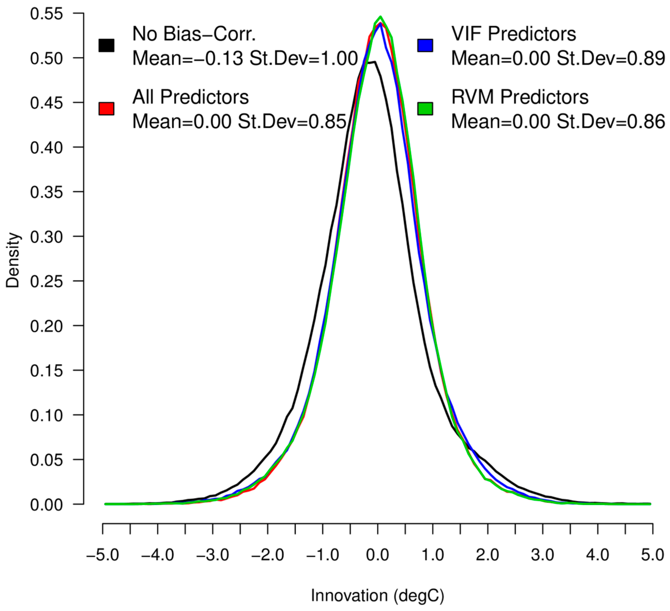
3.2. SST Bias Correction Scheme

In order to account for systematic biases of modeled and observed SST due to model and SST processing inaccuracies such as different diurnal variability, inexact air-sea fluxes, etc., a multi-linear bias model is formulated as such:

$$b={\beta }_0+{\displaystyle {\sum }_i}{\beta }_i{p}_i,$$

(1)

where $b$ is the modeled bias, ${\beta }_0$ is the constant offset, and ${\beta }_i$ and $p_i$ are the i-th bias coefficient and predictor, respectively. Equation (1) indeed combines several predictors simultaneously, which are weighted through the coefficients. Bias models like the latter are typically used within satellite radiance bias correction in Numerical Weather Prediction [46,47]. Using training data from free-running model simulations, the bias coefficients can be estimated through multi-linear regression and used in assimilation experiments to calculate the bias on-line, to be subtracted from the SST innovations. That is, a single innovation $d$ is given as $d=y-H\left(x^b\right)-b$, with $y$ as the SST observation and $H\left(x^b\right)$ as the background field equivalent, i.e., the model temperature at the first vertical model level, interpolated onto observation location. During the off-line calculation of the coefficients, multi-linear regression is performed, namely to find the $\beta$ coefficients that minimize ${\left(y-H\left(x^b\right)-b\right)}^2$ for the training data. The SST bias model can be later included in the variational cost function (VarBC) [48], although in this study, the bias is calculated prior to the cost function minimization and it is not updated due to the lack of enough “anchoring observations” [49] within each assimilation window in the Ligurian Sea. In the case of a rich in situ observing network, VarBC can be envisaged as well. The period from which training data are extracted partly overlaps with the experimental period (see Section 4.1). However, the set of bias coefficients is one for all the domain; namely, they do not change spatially, and training data are all used at once, thus preventing possible over-fitting problems in the cases of assimilating SST data already used to estimate the bias coefficients.

In applying Equation (1), relevant bias predictors for the bias of the innovations have to be identified. To this end, we have calculated the standardized regression coefficients [50] proposed by Auligné [51] for NWP applications: After normalizing the predictors (i.e., their mean value is subtracted and they are scaled by their standard deviation), the absolute values of the predictors’ coefficients indicate their weight in the bias correction scheme. Indeed, assuming Gaussian distribution for the predictors, a small coefficient indicates that the predictor has a small impact in the bias model and can eventually be disregarded. Sorting the coefficients’ absolute values thus provides an assessment of the predictors’ relevance. Large coefficients may however erroneously indicate a large weight in the bias scheme due to the collinearities and cross-correlation between predictors, although this does not necessarily imply numerical problems in the bias scheme [51].

Predictors are typically prognostic or diagnostic quantities extracted from the ocean model or atmospheric forcing and interpolated onto the observation locations, whose systematic error might be related to the systematic mismatch between observed and modeled SST. In particular, several predictors were evaluated, including sea surface salinity, mixed layer depth, solar and net heat fluxes, warm and cool skin layer temperature (i.e., $\delta T_{WL}$ and $\delta T_{CS}$), precipitation and evaporation, top 300 m ocean heat content, wind speed, fractional days (from 0 to 1 along each day), and their square values, in an attempt to characterize the bias as a function of the modeled air–sea flux exchange, upper ocean state, and skin SST sub-daily variability. Note that by doing this, there is no clear distinction between possible model or observation biases. Although the parameters are more representative of the model bias, the goal of this procedure is to correct the bias of the innovations without aiming at attributing it to the SEVIRI SST retrievals or the NEMO model systematic errors. Nonetheless, the latter can reasonably be considered more relevant, due to the under-estimation of the diurnal variability and possible inaccuracy in the surface boundary conditions and vertical mixing. For bias-correcting the SST observations only, better solutions exist, such as using reference (unbiased) data to estimate the satellite SST systematic errors [52].

In order to calculate the bias coefficients, innovations with all predictors interpolated onto the observation location were collected during the period from 15 September to 14 November 2017; namely the spin-up period is excluded. Performing multi-linear regression on normalized values of predictors and innovations yields the bar plot of Figure 4, where the absolute values of the regression coefficients are sorted in increasing order. The first four (smallest) coefficients are statistically non-significant and excluded from the bias model, while the remaining 19 form the group of predictors used later in the on-line bias correction. The largest weight comes from sea surface salinity, which is negatively correlated to the innovation bias, i.e., with decreasing salinity—and thus weak evaporation and low wind conditions—the difference between SEVIRI skin SST and model SST increases, confirming in turn that air–sea exchanges have a crucial impact on the SST bias.

Correlations and collinearity obviously exist between all of the bias predictors chosen, i.e., it is likely that the optimal set of predictors is smaller than the one actually used. Nevertheless, the correction scheme succeeds in reducing the bias. Two approaches have been investigated to assess the effect of reducing the set of predictors. First, we use the variance inflation factor (VIF) to estimate the collinearity of the predictors. VIF for the i-th predictor is defined as $VI{F}_i={\left(1-R_i^2\right)}^{-1}$, where $R_i^2$ is the coefficient of determination of the regression of all predictors except the i-th onto the i-th predictor [53]. VIFs are related to the diagonal elements of the inverse of the predictor correlation matrix. The larger VIFs are, the more collinearity affects the regression. In order to exclude collinear predictors, starting from the set of significant predictors, we exclude one-by-one the predictor with the largest VIF, until all VIFs are smaller than 10, which is a commonly used threshold in multi-linear regression [54]. The list of selected predictors is visible in Figure 4 (black squares). The VIF-based procedure yields 12 predictors, which in general retain the information about air–sea fluxes, skin SST layer, and mixed layer depth and heat content as in the all-predictor cases, but eliminate some quadratic or redundant parameters.

An alternative way to eliminate collinearity is through Relevance Vector Machine (RVM) [55], which is a machine learning technique to optimize regression by minimizing the set of predictors. It is also widely used for classification problems, and is based on Bayesian inference. We use a Gaussian kernel in the Karatzoglou et al. [56] implementation to obtain 11 relevance vectors. Figure 4 reports the predictors selected by RVM (orange squares). In general, the ones excluded by RVM are different from those excluded by VIF, although two of them overlap. Like for VIF, the relevant parameters for air–sea fluxes, skin SST layer, and sea surface characterization are retained, except for the ocean heat content, which is excluded.

Off-line results for the previously introduced bias correction scheme are summarized in Figure 5: The bias reduces the mean of the innovations from −0.13 to 0.00 °C and the innovations standard deviation from 1.00 to 0.85 °C, thus indicating a significant (15%) reduction. The selection of predictors through the VIF or RVM approach has very little impact on the resulting scores (standard deviation reduction equal to 0.89 and 0.86, respectively). For instance, the standard deviation of the differences of the bias corrections using all or only the RVM predictors is smaller than 0.09 °C. Therefore, in the following part of the manuscript, we will use the all-predictor bias correction scheme for the sake of simplicity.

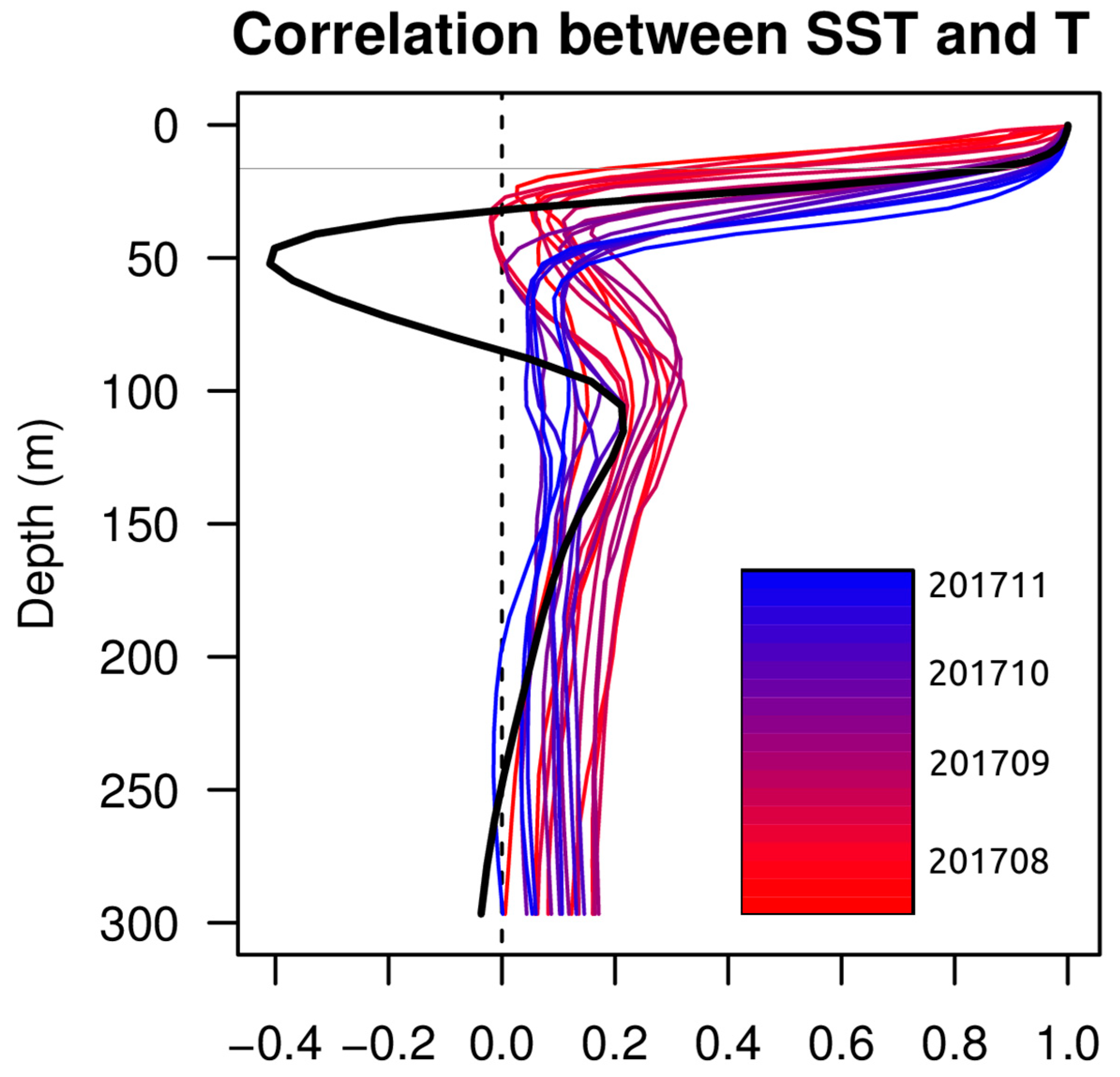
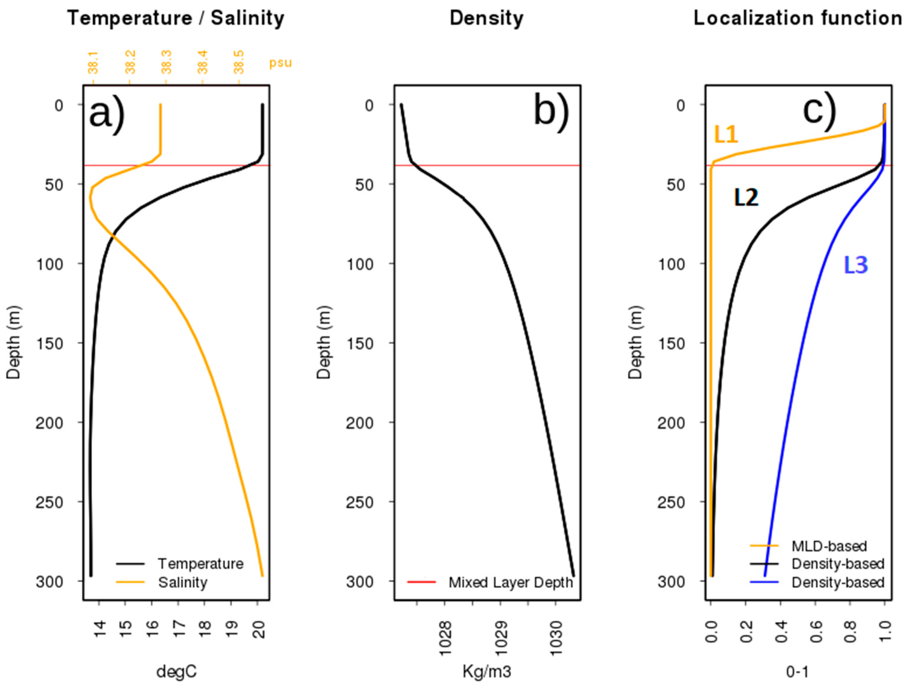
3.3. SST Vertical Localization

In order to assess the need of vertically localizing the SST data assimilation, here we formulate different localization functions, to be tested later within the experiments. The SST innovations can be thought of as providing relevant information about temperature in the mixed layer. Below the mixed layer depth, spurious vertical covariances may wrongly project the SST innovations, e.g., through spuriously long positive correlations or enhanced negative correlation right below the mixed layer depth (due to the rising/sinking of the mixed layer itself). Furthermore, misplacement of mixed layer depth, likely to occur when background-error covariances are calculated from a low-accuracy simulation, may further require localization, as well as in case of a small ensemble size for the ensemble-derived component of the background-error covariances. For instance, Chen et al. [5] report a positive impact by localizing SST observations within the mixed layer.

The vertical propagation of SST innovations is regulated by the vertical background-error auto-correlations, which are implied by the EOFs in our analysis system. Figure 6 exemplifies the vertical correlations between SST and temperature at depth, as reconstructed from both the stationary (black thick lines) and flow-dependent background-error covariances (red to blue thin lines, from August to mid-November 2017). The stationary covariances show a mixed layer depth located around 20 m of depth (thin grey line), with pronounced negative correlations in the thermocline (around 50 m of depth) and a reversed positive correlation at the base of the thermocline, decreasing with depth. Flow-dependent correlations show a deepening of the mixed layer with time, with a decrease with time of the reversed positive correlation right below the thermocline. Such vertical structures drive the vertical propagation of the SST observation at depth, and erroneous structures (such as overly negative or overly positive correlations below the mixed layer and the thermocline, respectively) may easily compromise the effectiveness of the SST data assimilation.

To this end, we investigate different formulations of a localization correlation function $L\left(z\right)$ between the first model level and the generic level $z$ to limit the deepening of the SST innovations. First, a strict criterion where the localization function gradually goes to zero in correspondence with the MLD is introduced:

$$\{\begin{array}{l}L(z)=1\\ L(z)=\frac{1}{2}\left[1-\cos \left(\pi \frac{d_m-d(z)}{d_m-d_0}\right)\right]\\ L(z)=0\end{array}\hspace{0.17em}for\hspace{0.17em}\begin{array}{l}for\hspace{0.17em}d(z)\le d_0\\ \hspace{0.17em}{d}_0<d(z)<d_m\\ for\hspace{0.17em}d(z)\ge d_m\end{array}$$

(2)

where $d\left(z\right)$ is the depth, $d_m$ is the MLD, and $d_0$ is a near-surface depth representing the foundation SST (here chosen to be equal to 10 m of depth). We hereafter refer to this localization scheme as L1.

More gentle criteria may be adopted based on the density and using a Gaussian decay with depth:

$$L\left(z\right)=\exp \left[-\frac{1}{2} \frac{{\left({\rho }_0-\rho \left(z\right)\right)}^2}{\beta \Delta {\rho }_{500}}\right]$$

(3)

where ${\rho }_0$ is a surface reference density (here taken at the first model level), $\Delta {\rho }_{500}$ quantifies the vertical variability of the density, i.e., the maximum of density difference with respect to ${\rho }_0$ within the top 500 m. $\beta$ is a parameter regulating the decay of the localization function. Figure 7 shows profiles of temperature salinity and density with corresponding mixed layer depth, and three localization functions: One for (2) and two for (3), with two different values of $\beta$ (equal to 1/16 and 1/4, and referred to as L2 and L3 hereafter, respectively). While the MLD-based localization function concentrates the impact of SST data in the top 10–20 m and rapidly decreases to 0 at MLD, the other two density-based localization functions result in a deeper propagation of the SST data that differently decrease to 0, in the first case at around 150–200 m of depth, while in the second below 300 m of depth. These formulations of the vertical localization respond indeed to different strategies: In the first case, minimum vertical propagation is imposed in order to correct only the near-surface temperature. In the other two cases, SST data are allowed to modify the mixed layer and the levels immediately below, although the penetration of the SST innovations is attenuated with the depth.

The previously described localization functions can be generalized for any pair of vertical levels in order to form the symmetric localization correlation matrix $L$, where each element $L_{ij}$ contains the correlation between levels $i$ and $j$. This matrix is evaluated on-line in the variational code. MLD and density fields used in (2) and (3), respectively, are taken from the background fields (for the MLD, the definition in Section 2 is used). The localization function is applied to the control vector following the formulation in Buehner [57] and Wang et al. [58], where the squared-root background-error covariance matrix is redefined to account for the correlation matrix used for covariance localization. Formally, consider the vertical square-root covariance matrix $V_v$ such that the vertical component of the background-error covariance matrix equal to $B_v=V_v{V}_v^T=U\mathsf{\lambda } {\left(U\mathsf{\lambda }\right)}^T$, with $U$, the matrix whose columns contain the eigenvectors, and $\mathsf{\lambda }$, the diagonal matrix whose elements are the square-root eigenvalues of $B_v$ (also see the Appendix A). The localized matrix $\widetilde{V_v}$ is then defined as:

$$\widetilde{V_v} =\left[\mathrm{diag}\left(U_{\mathbf{1}}{\mathsf{\lambda }}_{\mathbf{1}}{L}^{\frac{\mathbf{1}}{\mathbf{2}}}\right), \dots , \mathrm{diag}\left(U_k{\mathsf{\lambda }}_k{L}^{\frac{\mathbf{1}}{\mathbf{2}}}\right), \dots ,\mathrm{diag}\left(U_K{\mathsf{\lambda }}_K{L}^{\frac{\mathbf{1}}{\mathbf{2}}}\right)\right]$$

(4)

where $\mathrm{diag}(\dots )$ is the diagonal matrix that contains the vector $(\dots )$ on the diagonal elements, and the subscript $k$ indicates the $k$-th eigenvalue and eigenvector. In a way similar to Buehner [57], it can be demonstrated that $\widetilde{V_v}{\left(\widetilde{V_v}\right)}^T=B_v\ast L$, with $\ast$ being the Schur product (or entry-wise product).

In the future, the adoption of multiple outer loops in the analysis scheme might be envisaged in order to refine the localization function definition within the successive outer loops, although this strategy is not explored here.

4. Experimental Setup and Results

4.1. Configuration of the Experiments

We introduce here the experiments performed to assess the impact of SST data assimilation with the novelties presented above. Experiments are summarized in

Table 1. List of experiments performed and characteristics of the SST assimilation scheme. The localization functions are: MLD as in Equation (2); DEN1 (density based) as in Equation (3) with $\beta$ equal to 1/16; DEN2 as in Equation (3) with $\beta$ equal to 1/4.

Experiment	SST Assimilation	SST Data	Method	Localization
CT	NO	-	-	-
CR	Nudging	L4 (Foundation)	1st Level	-
S1	Hybrid 3DVAR	Night-time SEVIRI	1st Level	NO
S2	Hybrid 3DVAR	All-day SEVIRI	1st Level	NO
S3	Hybrid 3DVAR	All-day SEVIRI	1st Level + bias correction	NO
S4	Hybrid 3DVAR	All-day SEVIRI	Warm layer skin SST	NO
S3L1	Hybrid 3DVAR	All-day SEVIRI	1st Level + bias correction	MLD (L1)
S3L2	Hybrid 3DVAR	All-day SEVIRI	1st Level + bias correction	DEN1 (L2)
S3L3	Hybrid 3DVAR	All-day SEVIRI	1st Level + bias correction	DEN2 (L3)
S4L1	Hybrid 3DVAR	All-day SEVIRI	Warm layer skin SST	MLD (L1)
S4L2	Hybrid 3DVAR	All-day SEVIRI	Warm layer skin SST	DEN1 (L2)
S4L3	Hybrid 3DVAR	All-day SEVIRI	Warm layer skin SST	DEN2 (L3)

. In addition to a control run (CT) without any data ingestion and the run with relaxation to SST data (CR, see later on for the choice of the relaxation coefficient), the S1 and S2 experiments assimilated SEVIRI SST retrievals in the hybrid ensemble-variational scheme. However, S1 assimilated only nighttime measurements (from 10 pm to 4 am), while S2 also assimilated daytime measurements (all available SST data). S1 thus represents the conservative standard method, used currently in most analysis systems [8]. Starting from the S2 baseline experiment setup, the bias correction scheme introduced in Section 3.2 was tested in the S3 experiment, while in the S4 experiment, the model SST plus the warm layer scheme was used to calculate the innovations (i.e., $d=y-H\left(x^b\right)-\delta T_{WL}$), in order to test the analytical inclusion of the skin layer diurnal warming. Finally, the three localization functions L1, L2, and L3 were combined with S3 and S4 to form the six respective additional experiments. The three localization functions correspond to the application of Equation (2) or Equation (3) with values of $\beta$ equal to 1/16 and 1/4, respectively. Note that in order to test the assimilation of SST data alone and have independent verifying data, only SST observations were assimilated in these experiments, i.e., no altimetry nor in situ data are assimilated.

For all S experiments, the observational error for SST (${\epsilon }_{SST}$) data is set equal to

$${\epsilon }_{SST}=\gamma \sqrt{i^2+r{\left(i,j\right)}^2}=\frac{1}{\exp (-\frac{\delta t^2}{T^2})}\sqrt{i^2+r{\left(i,j\right)}^2},$$

(5)

where $i^2$ is the instrumental error variance (set equal to 0.4 °C according to the product specification [37]), $r{\left(i,j\right)}^2$ is a spatially varying representativeness error variance, estimated through the method proposed by Oke and Sakov [59] and small for the Ligurian Sea region (about 0.05 °C on the average). The multiplicative term $\gamma$ increases the root-squared sum of instrumental and representativeness error by accounting for the interval between observation and analysis time ($\delta t$) through an exponential decay (with length-scale $T$ equal to 3 days), which accounts for the temporal representativeness of the observations considering their time lag with respect to the analysis time, due to the three-dimensional formulation of the data assimilation, similarly to Oke et al. [60]. In practice, the total observational error ${\epsilon }_{SST}$ used in the experiments ranges between 0.40 and 0.45 °C, based on the above equation.

The CR experiment relaxes the model SST towards the L4 SST analysis from CNR (Consiglio Nazionale delle Ricerche) [61], which ingests nighttime measurements collected by infrared sensors onboard different satellite platforms. In order not to strongly relax to this product during daytime, a sinusoidal function for the relaxation coefficient $\beta \left(t\right)$ is used:

$$\beta \left(t\right)=\frac{\delta Q}{\delta T}={\mathsf{\beta }}_0\left\{\left[1+\sin \left(\frac{\left(1-s_t\right) \pi }{86400}\right)\right]\left(1-\alpha \right)+\alpha \right\}$$

(6)

where ${\mathsf{\beta }}_0$ is the nighttime relaxation coefficient (equal to −60 W m⁻² K⁻¹), $s_t$ are the seconds from the beginning of the day at time $t$, and $\alpha$ is the fractional parameter denoting the percentage of relaxation coefficient at noon (equal to 0.2, i.e., 20%, in our experiments). In practice, the relaxation coefficient smoothly decreases to −12 W m⁻² K⁻¹ at noon, following the sinusoidal shape in order to give less weight to the nudging during daytime. The tuning of these parameters was performed in previous experiments [20]. More sophisticated relationships for $\beta \left(t\right)$ could also be formulated (e.g., as a function of wind speed to decrease the relaxation in conditions of large skin SST warming, or to the MLD to modulate the propagation as a function of the ocean stratification) but are not considered here, where the aim is to compare a standard form of SST nudging to variational data assimilation of daytime SST data.

Finally, it should be noted that the bias correction coefficients were calculated from free-running model dataset collecting bias and predictor data for the period from 15 September to 14 November 2017, while the assimilation experiments were run for the period from 2 August to 14 November 2017. Thus, there exists a temporal overlap between the period of the bias training data and the validation period; namely, validation data are not independent from those used to train the bias correction scheme. However, the bias correction scheme is here conceived as a running (flow-dependent) adaptive bias retuning; therefore, the overlap mimics a real-time operational system.

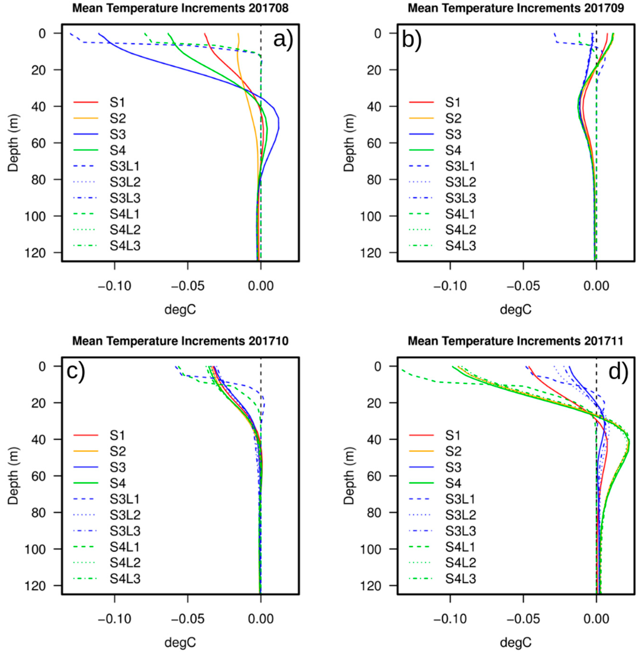
4.2. Analysis Increments, Mean Ocean State, and Diurnal Variability

We start the assessment of the experiments by looking at the analysis increments for the assimilative experiments that were previously introduced. Figure 8 shows the area and monthly averaged temperature analysis for the four different months during the experimental period, namely corresponding to monthly means of the analysis increments. The impact of SST observations appears strong during the first month, with up to −0.1 °C at the surface. The experiment with bias correction (S3) provides the largest increments, while the one without bias-correction (S2) provides the smallest ones, and S1 and S4 provide intermediate increments. Thus, the application of bias correction amplifies the impact of the SST retrievals near the surface. The fact that the off-line estimation of the bias coefficient does not use data from August may also contribute to having such large increments. The use of the L1 localization amplifies the impact over the top 5 m, below which increments abruptly vanish. For S3, a slight positive increment is visible below the mixed layer, which implies in turn a sharper thermocline, generally absent in the other experiments. For the successive months, the effect of the SST assimilation changes: During September, there is a slight and persisting cooling that contributes to a further rise in the MLD, likely due to the overestimated seasonal deepening of the MLD itself in the control experiments. The experiments with L1 localization behave differently; namely, the SST provides large surface negative increments, as the increments in the previous month were not propagated enough below the near-surface ocean. The last two months have qualitatively similar profiles of analysis increments, which tend to maintain, to a different extent, the upper ocean cooling that the SST data assimilation leads to, raising the MLD, and in November, further sharpening the thermocline. During the last month, the impact of L2 and L3 localization is also visible. Salinity analysis increments are negligible and not shown, peaking at 0.004 psu of positive increments near the mixed layer depth. This implies that the sea surface salinity, while playing a significant role in the SST bias-correction scheme presented in Section 3.2 (see Figure 4) as a proxy of air–sea flux variability, does not hold large cross-covariances with sea surface temperature in the current analysis scheme.

The effect of the SST data assimilation on the long-term mean ocean state is shown in Figure 9 in terms of SST and MLD differences with respect to the control run (CT). For simplicity, we limit the assessment to the experiments S1 (traditional nighttime only assimilation) and S3 (all-data assimilation with bias correction), with the other experiments S2 and S4 providing intermediate patterns. In both S1 and S3, the SST data lead to a cooling in a large part of the domain, peaking at about −1.0°C and −1.6 °C, respectively, in the western area. Consistently with the analysis increments, the S3 setup amplifies the impact of SST data. There exist areas of neutral to slightly positive SST warming (up to 0.2 °C in S3) in the eastern area. The corresponding MLD shows a rise that occurs mostly in the basin, peaking at −12 m (S1) and −20 m (S3) in the western part of the domain. The assimilation of night-only observations prevents the rising of the mixed layer and exhibits a deepening of the mixed layer in the Gulf of Genoa (northern part of the domain up to 15 m).

In Figure 10, diurnal amplitudes from selected experiments are compared in the observation space for comparison with SEVIRI data (see the figure caption for details on the calculation). The comparison suggests that the (sub-skin) SST amplitude is strongly under-estimated with respect to the SEVIRI-derived data, even though the warm layer temperature increment was added to the model data. Assimilating nighttime data (S1) increases the amplitude in the western part of the domain, while the addition of daytime measurements (S2) further increases the amplitude. The assimilation of nighttime SST observations with either bias correction (S3) or warm-layer-based correction (S4) greatly improves the comparison against satellite data. It is worth noting that the assimilation scheme is three-dimensional; namely, observations are assumed to be simultaneous during the variational minimization, so that the impact of the observations on the diurnal variability is not a direct consequence of the observation ingestion, but caused by the additional variability induced by the analysis increments. Furthermore, the localization L1 strongly limits the impact of the observations on the diurnal amplitude, suggesting that the corrections within the entire mixed layer and below are responsible for the enhanced diurnal amplitudes.

4.3. Validation against Independent Data

4.3.1. Validation against Glider Data

The SST data assimilation experiments were first validated against SST nighttime measurements from SEVIRI and independent altimetry data (not shown). As expected, experiments with the assimilation of SEVIRI data all show a significant improvement with respect to the control experiment, leading to negligible bias and SST Root Mean Square Error (RMSE) improvements of the order of 11–14% and 3–10% at day 1 and 3 of the forecasts, respectively. Such SST validating data are not independent and are not discussed further. Regarding the validation against altimetry data, differences of RMSE among the experiments are of the order of 1–2%. They are not shown or discussed further since their results are not statistically significant.

We used independent data from the two gliders deployed during the LOGMEC17 sea trial to validate against the independent dataset of the experiments previously introduced. The glider tracks are shown in the top left panel of Figure 3, and were designed to follow some altimetry tracks in order to provide co-located information about sea surface height and sub-surface density fields [20]. Glider tracks cover a relatively extended area of the domain, and are thus the primary dataset for validating the SST data assimilation. The validation was initially conducted on the mixed layer depth (see definition in Section 2). First, we show the day-by-day and hourly temporal variability of the area-averaged MLD for the experiments (Figure 11a,b) during the validation period (model space). At the end of September, the shallow MLD is similar between the experiments, except for CT and CR showing slightly deeper MLD than that of the others. During October and November, the MLD sinks and the differences between the experiments amplify. In particular, S3 (together with S3L2 and S3L3) exhibits the shallowest MLD among the experiments. S4 (with S4L2 and S4L3) and S2 show slightly deeper MLD than that of S3. Finally, the experiments with strong MLD-based localization and the CT and CR control experiments have the shallowest MLD, suggesting that such a localization strategy does not allow for MLD corrections. To summarize, assimilating SEVIRI SST observations enables thinning of the mixed layer, which is even stronger when daytime measurements are assimilated and when the bias-correction of SST data is switched on. Density-based localization procedures do not have a large impact on the MLD variability, while the strong criterion based on the background MLD significantly reduces the effect of the SST data on the MLD thinning. The MLD versus the time of the day shows very similar diurnal amplitudes between the experiments, with the deepest MLD occurring before sunrise and the shallowest at around 15 UTC.

The bottom panel of Figure 11c shows the time series—as does the top left panel—but in observation space and with MLD calculated from glider profiles as well, using in both cases the 0.125 kg m⁻³ density criterion described in Section 2. Data are 10 day averages in order to filter out the large high-frequency (i.e., sub-daily) variability present in the raw data. MLD values from the two gliders during the 10 day windows are combined together through arithmetic average, and the same procedure is followed for the model data after interpolation onto glider locations. Standard deviations of the observed values are also reported in the plot. The plot confirms the previous finding; namely, experiments S3 and S4 and their combination with the L2 and L3 localization lead to a shallower mixed layer. These latter experiments are in much closer agreement with the data from the gliders. On the contrary, control experiments and L1 localization show an enhanced deepening of the mixed layer towards November. Quantitative validation of the MLD is summarized in

Table 2. Skill score statistics (bias as model minus observations and RMSE), both in meters) in MLD space versus glider profile data from LOGMEC17. The RMSE column reports the percentage reduction of RMSE with respect to CT experiment in parentheses.

Experiment	MLD Bias (m)	MLD RMSE (m)
CT	6.9	11.2
CR	6.7	11.4 (−1.8%)
S1	4.4	10.9 (2.7%)
S2	−0.3	9.5 (15.2%)
S3	0.2	8.9 (20.5%)
S4	0.3	9.0 (19.6%)
S3L1	5.0	10.5 (6.2%)
S3L2	−1.6	9.0 (19.6%)
S3L3	−0.1	8.6 (23.2%)
S4L1	6.6	11.2 (0.0%)
S4L2	0.4	9.9 (11.6%)
S4L3	−0.4	8.8 (21.4%)

, which reports bias and RMSE versus the MLD calculated from the glider profiles. Scores are calculated from the third day of forecasts in order to highlight the predictive skills of the system, although results from day 1 and 2 are close to those shown. Reduction of bias and RMSE is largest in S3 compared to S1, S2, and S4, while the control experiments (CT and CR) show a large bias of about 7 m. SST relaxation does not provide significant improvements, while nighttime-only data assimilation results in a 4.4 m bias. Experiments S2, S3, and S4 all have a bias close to 0. The use of L3 density-based vertical localization (in S3L3 and S4L3) further improves the skill scores compared to the corresponding experiments without localization (S3 and S4, respectively), indicating the positive impact of this scheme in predicting MLD variability. The experiment S3L3 yields the best skill scores, with bias and RMSE equal to −0.1 and 8.6 m, respectively, the latter corresponding to a 23.2% improvement of RMSE compared to the control experiment CT.

More common validation of temperature and salinity profiles was performed against the glider data for both analyses and forecasts. Figure 12 shows profiles of temperature bias against the glider profiles for the top 150 m. The warm bias present in CT is mitigated in CR only at the surface (top 20 m), while it worsens around 50 m of depth. The sole assimilation of nighttime measurements (S1) or the strong localization (S3L1, S4L1) do not substantially modify the vertical structure of the bias, while all other experiments (S3, S4, and the corresponding ones with localization L2 and L3) significantly reduce the bias in the top 100 m of depth, with particularly unbiased temperature profiles from S3L2, S3L3, and S4L3, suggesting that the density-based localization helps reduce the upper ocean bias.

Skill score statistics (RMSE) are first assessed as a function of the hour of the day (Figure 13) and then as a function of vertical layer (Figure 14). In particular, Figure 13 shows the RMSE against glider data in the top 10 m as a function of 3 h time intervals during the first day of forecast. The relaxation experiment leads to a small improvement of the order of 0.1 °C, rather uniform over the time of the day. S1 and S2 provide similar results, with an error of about 0.45 °C (averaged over time), and increasing after 18 UTC. The experiment S3 provides the best skill scores, with minimum scores around noon, while the S4 experiment provides scores worse than S1 and S2 between 11 and 15 UTC, confirming that a mismatch between the diagnostic warm layer and the observed one exists during these hours. The experiments with localization and bias correction suggest that localization does not improve results in this near-surface layer. Moreover, combining this validation with the diurnal amplitude assessment (Figure 10) suggests that the experiment S3 improves the representation of the diurnal cycle, acting on the increase of the surface temperature between around 8 and 18 UTC. Note that there is no significant correlation between the RMSE as a function of the time of the day and the number of hourly observations (bottom panel of Figure 2) either in the CT nor in the SST assimilation experiments, meaning that the statistics are representative of the actual change of accuracy during the day.

Figure 14 shows the temperature RMSE decrease with respect to CT for all of the experiments and for the forecasts at days 1 and 3, generally confirming the previous findings. Scores were divided into three layers, accounting for mixed layer, between mixed layer and thermocline depths, and below—down to 300 m (see the figure caption for details). The relaxation (CR experiment) provides only very small improvements of below 10% above the thermocline depth and statistically insignificant below. The improvements in the mixed layer are large for the assimilative experiments (above 32%) and at maximum for S3 (RMSE decrease around 47% and 43% at days 1 and 3 of forecasts, respectively). Below the mixed layer depth, S3 and S4 show the largest impact, while the L1 localization nullifies the SST data assimilation to a great extent. It is also evident that nighttime-only data assimilation (S1) does not provide an impact as large as those of the other experiments. Below the thermocline depth, the L2 and L3 localization boost the scores of the S3 and S4 experiments, suggesting that this procedure appears relevant for deep ocean results. The nighttime-only SST assimilation experiment (S1) shows a negative impact at day 1 and is neutral below the thermocline at day 3, suggesting that the enhanced representativeness error associated with nighttime data for the day after upper ocean vertical structure may have a detrimental effect on the thermocline shape. In the large majority of SST assimilation experiments, more improvements are shown at day 3 than at day 1 below the mixed layer; namely, the impact of SST observations is amplified with the forecast range within the vertical region characterized by the largest variability (i.e., between the mixed layer depth and the end of the thermocline).

4.3.2. Validation against Mooring and Drifter Data

Additional validation of the SST data assimilation experiments was performed against data from the oceanographic and meteorological moored buoys deployed during the LOGMEC campaign (see Figure 3a for their location). The buoys were equipped with CTD sensors. The oceanographic buoy covers unevenly spaced depths between 30 and 1015 m of depth, while the meteorological one covers between 10 and 105 m of depth. The upper ocean temperature comparison is shown in Figure 15 (panel a) and confirms the ability of the experiment S3 in correctly raising the mixed layer and thermocline depths with respect to control or nighttime-observation-only experiments. Although at the buoy location, the model warm bias is very large, the optimal assimilation of SEVIRI SST retrievals significantly mitigates this bias. Consistently, the RMSE versus the oceanographic buoy data (Figure 15, panel b) is significantly reduced, from more than 3 °C (CT and CR) to about 1.7 °C (S3). In this comparison, the experiment with bias correction also proves to be the most effective one in reducing systematic errors. The localization L2 in S3L2 further improves the RMSE scores between approximately 50 and 100 m of depth. In the comparison against the meteorological buoy, it turns out that upper ocean temperatures (top 20 m, i.e., the mixed layer) are best captured by experiments S4 and S4L1. Along the thermocline, experiments S1 and S2 perform better than others, suggesting that in this shallow and coastal region, the changes induced by the experiments S3 and S4 regarding the mixed layer depth and thermocline locations are probably not optimal.

Assessing how the assimilation of SST induces changes in the surface circulation is non-trivial. Here, we compare the surface current speed and direction from the experiments against observed current data derived from drifters deployed during the LOGMEC campaign, which are visible as yellow tracks in the bottom panels of Figure 16. Drifter velocity data were obtained through centered differences of drifter positions at a 10 min frequency and successively low-pass filtered with 6 h cut-off time-windows. The data cover the eastern area of the domain. The validation of the current speed (RMSE, panels a and b of Figure 16) indicates that all experiments ingesting SST data improve the score significantly compared to the control experiment CT. The SST relaxation (CR) has a neutral impact on the sea surface current speed. The experiment S4L2 leads to the greatest RMSE decrease (18%). The validation of the sea surface current direction (top right panel) indicates that the experiment S4L3 is the best performing one; all experiments provide significant improvement with respect to CT, except that with SST relaxation and those with L1 vertical localization. For some experiments, the impact of SST assimilation on current speed and direction appears inconsistent, likely due to the stretching effect of current systems such as gyres in the southeastern part of the domain.

The middle and bottom panels of Figure 16c–f show the mean surface circulation during the validation period for CT, S1, S3, and S4L2. From these, one can deduce that the improvement is due to multiple factors. The southward current detaching from the Liguro-Provencal current off of Tuscany is visible only in the experiments with SST data assimilation and, in particular, the S4L2 seems to reproduce this current in close agreement with the drifter trajectories (southward displacement). Furthermore, the gyre circulation present in CT around Capraia Island (northeast of Sardinia) is largely damped in the assimilative experiment. Assimilating only nighttime data (S1) does not exhibit this structure, while S3 and S4L2 show the gyre edge in agreement with the drifter trajectories. It should also be noted that in the northern part of the domain, the experiments S3 and S4L2 show an enhanced Liguro-Provencal current that flows west off of Sardinia and then follows the western Ligurian and French coast, which is weakened and moved westwards in the CT and S1 experiments. This suggests that assimilating SEVIRI data has a profound impact on the upper ocean circulation, although the lack of validating current data in the western part of the domain prevents us from understanding whether the intensification of the Liguro-Provencal current and the shift of the French branch of the Liguro-Provencal current is realistic.

5. Summary and Discussion

In this work, we have investigated several ways to assimilate daytime SST data from infrared sensors in order to obtain optimal sub-surface corrections for correctly modulating the mixed layer thickness. A regional ocean prediction system that covers the Ligurian Sea and consists of the NEMO ocean model and a hybrid ensemble-variational data assimilation scheme is used to assess the potential impact of SEVIRI SST retrievals. Optimally assimilating SST observations is a long-standing problem in operational regional ocean prediction systems, because (i) a mismatch between the SST measured by satellite sensors (skin or sub-skin SST) and the SST from models (first model level generally between 0.3 and 1.0 m) exists, the latter under-estimating the diurnal cycle; (ii) the vertical propagation of the SST innovations is driven by the background-error covariances, which may embed spurious or overly smoothed correlation profiles, misplaced thermocline, or invariant structure, thus inducing an incorrect response of the forecast model below the upper ocean; (iii) using three-dimensional assimilation schemes (without the time dimension) does not guarantee that innovations collected during the daily or multi-daily time-window are correctly ingested into the analysis. Nevertheless, correctly ingesting SST data has the potential to improve the upper ocean structure, especially because SST retrievals are available from many satellite missions, thus potentially covering areas with a lack of in situ data. Using daytime data may also recover from nighttime cloudy conditions that significantly reduce the number of SST retrievals from infrared sensors for data assimilation.

In order to evaluate possible improvements of the SST assimilation scheme to account for under-estimated diurnal amplitude in ocean models, we propose either a skin temperature and air–sea flux aware bias correction scheme or a modification of the observation operator to account directly for the sub-skin temperature in the innovation computation. The sub-skin temperature warming was taken from a prognostic model embedded in the NEMO ocean model. Results suggest that the bias correction that uses parameters related to air–sea fluxes, skin layer temperature, and time of the day as predictors provides the best forecast skill scores. This is likely due to (i) the systematic errors of the warm layer model together with the systematic errors of the SEVIRI data calibration, which the bias-correction scheme reduces by construction and (ii) systematic errors in the atmospheric forcing and bulk formulas, which are reduced, including air–sea flux predictors in the bias correction scheme. It should be noted, however, that also using the warm-layer-based observation operator provides improvements with respect to the case of simply using the first model level. All of the assimilation experiments help reduce the upper ocean (top 90 m) temperature error and the deep MLD bias, including the experiment that simply calculated the innovations from the first model level.

Vertical localization appears generally marginal, and strong conclusions about the optimal configuration depend on the specific application and target accuracy. A sharply decaying localization function (i.e., the one based on MLD, Equation (2)) generally worsens all of the skill scores; in particular, it is not able to shift the mixed layer depth and thermocline. More gentle localization functions than the latter, based on density criteria, are able in turn to improve the MLD skill scores, providing the least unbiased forecasts of MLD, with slight improvements of skill scores below the mixed layer.

Another finding of this work is that using a relaxation scheme has only a marginal impact at the surface (top 20 m), while below, it even worsens the results. Relaxation clearly emerges as a sub-optimal procedure for ingesting SST data, although it can be implemented in a more sophisticated way (e.g., relaxation coefficient inversely proportional to the MLD, or decreased during daytime for low-wind conditions). However, it is not straightforward to account for the sub-diurnal variability when one uses daily gap-filled satellite SST products within relaxation schemes. Finally, we evaluated the impact of SST data without assimilating other measurements. This was a challenging experimental configuration used to assess the net impact of the data. However, it should be noted that combining the SST data assimilation with in situ profiles and altimetry should be able to further improve the skill scores, as in situ profiles in particular provide anchoring information to modulate the vertical structure of temperature and, in particular, shift the mixed layer base. Our experiments also suggest that in areas where the in situ observing network is fundamentally missing for geographical or economic reasons, it is worthy to implement optimal data assimilation schemes for ingesting satellite data such as SST, as they lead to significant improvements of the short-range forecasts.

By extensively validating the experiments with independent data collected during the LOGMEC17 observational campaign, we have shown that even a simple but well-tuned multi-linear bias correction scheme is able to improve the upper ocean structure and the diurnal variability, even adopting three-dimensional data assimilation schemes. The results promisingly foster the use of daytime SST data from infrared sensors within operational oceanographic forecasts. The hybrid ensemble-variational paradigm offers a relatively easy way to modulate the vertical background-error covariances over time, as they drive the vertical propagation of the surface observations and whose correct characterization is crucial for SST data assimilation.

References

1. Le Traon, P.Y. Satellites and Operational Oceanography. In Operational Oceanography in the 21st Century; Schiller, A., Brassington, G.B., Eds.; Springer: Dordrecht, The Netherlands, 2011; pp. 29–54. [Google Scholar] [CrossRef]
2. Oke, P.R.; Larnicol, G.; Jones, E.M.; Kourafalou, V.; Sperrevik, A.K.; Carse, F.; Tanajura, C.A.S.; Mourre, B.; Tonani, M.; Brassington, G.B.; et al. Assessing the impact of observations on ocean forecasts and reanalyses: Part 2, Regional applications. J. Oper. Oceanogr. 2015, 8, s63–s79. [Google Scholar] [CrossRef]
3. Legler, D.M.; Freeland, H.J.; Lumpkin, R.; Ball, G.; McPhaden, M.J.; North, S.; Crowley, R.; Goni, G.J.; Send, U.; Merrifield, M.A. The current status of the real-time in situ Global Ocean Observing System for operational oceanography. J. Oper. Oceanogr. 2015, 8, s189–s200. [Google Scholar] [CrossRef]
4. Miyazawa, Y.; Varlamov, S.M.; Miyama, T.; Guo, X.; Hihara, T.; Kiyomatsu, K.; Kachi, M.; Kurihara, Y.; Murakami, H. Assimilation of high-resolution sea surface temperature data into an operational nowcast/forecast system around Japan using a multi-scale three-dimensional variational scheme. Ocean Dyn. 2017, 67, 713–728. [Google Scholar] [CrossRef]
5. Chen, Y.L.; Yan, C.X.; Zhu, J. Assimilation of sea surface temperature in a global Hybrid Coordinate. Ocean Model. Adv. Atmos. Sci. 2018, 35, 1291–1304. [Google Scholar] [CrossRef]
6. Liu, Y.; Fu, W. Assimilating high-resolution sea surface temperature data improves the ocean forecast potential in the Baltic Sea. Ocean Sci. 2018, 14, 525–541. [Google Scholar] [CrossRef]
7. Helber, R.W.; Barron, C.N.; Carnes, M.R.; Zingarelli, R.A. Evaluating the sonic layer depth relative to themixed layer depth. J. Geophys. Res. 2008, 113, C07033. [Google Scholar] [CrossRef]
8. Waters, J.; Lea, D.J.; Martin, M.J.; Mirouze, I.; Weaver, A.; While, J. Implementing a variational data assimilation system in an operational 1/4 degree global ocean model. Q. J. R. Meteorol. Soc. 2015, 141, 333–349. [Google Scholar] [CrossRef]
9. Storto, A.; Masina, S. C-GLORSv5: An improved multipurpose global ocean eddy-permitting physical reanalysis. Earth Syst. Sci. Data 2016, 8, 679–696. [Google Scholar] [CrossRef]
10. Marullo, S.; Santoleri, R.; Ciani, D.; le Borgne, P.; Péré, S.; Pinardi, N.; Tonani, M.; Nardone, G. Combining model and geostationary satellite data to reconstruct hourly SST field over the Mediterranean Sea. Remote Sens. Environ. 2014, 146. [Google Scholar] [CrossRef]
11. Gentemann, C.L.; Donlon, C.J.; Stuart-Menteth, A.; Wentz, F.J. Diurnal signals in satellite sea surface temperature measurements. Geophys. Res. Lett. 2003, 30, 1140. [Google Scholar] [CrossRef]
12. Marullo, S.; Minnett, P.J.; Santoleri, R.; Tonani, M. The diurnal cycle of sea-surface temperature and estimation of the heat budget of the Mediterranean Sea. J. Geophys. Res. Ocean. 2016, 121, 8351–8367. [Google Scholar] [CrossRef]
13. Donlon, C.J.; Martin, M.; Stark, J.; Roberts-Jones, J.; Fiedler, E.; Wimmer, W. The Operational Sea Surface Temperature and Sea Ice Analysis (OSTIA) system. Remote Sens. Environ. 2012, 116, 140–158. [Google Scholar] [CrossRef]
14. GHRSST. Available online: https://www.ghrsst.org/ghrsst-data-services/products (accessed on 19 November 2019).
15. While, J.; Mao, C.; Martin, M.J.; Roberts-Jones, J.; Sykes, P.A.; Good, S.A.; McLaren, A.J. An operational analysis system for the global diurnal cycle of sea surface temperature: Implementation and validation. Q. J. R. Meteorol. Soc. 2017, 143, 1787–1803. [Google Scholar] [CrossRef]
16. Akella, S.; Todling, R.; Suarez, M. Assimilation for skin SST in the NASA GEOS atmospheric data assimilation system. Q. J. R. Meteorol. Soc. 2017, 143, 1032–1046. [Google Scholar] [CrossRef] [PubMed]
17. Gentemann, C.L.; Akella, S. Evaluation of NASA GEOS-ADAS modeled diurnal warming through comparisons to SEVIRI and AMSR2 SST observations. J. Geophys. Res. Ocean. 2018, 123, 1364–1375. [Google Scholar] [CrossRef]
18. Korres, G.; Denaxa, D.; Jansen, E.; Mirouze, I.; Pimentel, S.; Tse, W.H.; Storto, A. Assimilation of SST data in the POSEIDON system using the SOSSTA statistical-dynamical observation operator. Ocean Sci. Discuss. 2019. [Google Scholar] [CrossRef]
19. Jansen, E.; Pimentel, S.; Tse, W.H.; Denaxa, D.; Korres, G.; Mirouze, I.; Storto, A. Using Canonical Correlation Analysis to produce dynamically-based highly-efficient statistical observation operators. Ocean Sci. 2019, 1023–1032. [Google Scholar] [CrossRef]
20. Storto, A.; Oddo, P.; Cozzani, E.; Coelho, E.F. Introducing along-track error correlations for altimetry data in a regional ocean prediction system. J. Atmos. Ocean. Technol. 2019. [Google Scholar] [CrossRef]
21. Oddo, P.; Storto, A.; Dobricic, S.; Russo, A.; Lewis, C.; Onken, R.; Coelho, E. A hybrid variational-ensemble data assimilation scheme with systematic error correction for limited-area ocean models. Ocean Sci. 2016, 12, 1137–1153. [Google Scholar] [CrossRef]
22. Storto, A.; Oddo, P.; Cipollone, A.; Mirouze, I.; Lemieux, B. Extending an oceanographic variational scheme to allow for affordable hybrid and four-dimensional data assimilation. Ocean Model. 2018, 128, 67–86. [Google Scholar] [CrossRef]
23. Storto, A.; Falchetti, S.; Oddo, P.; Jiang, Y.M.; Tesei, A. Assessing the Impact of Different Ocean Analysis Schemes On Oceanic and Underwater Acoustic Predictions. J. Geophys. Res. Ocean. 2019. in review. [Google Scholar]
24. Dobricic, S.; Pinardi, N. An oceanographic three-dimensional assimilation scheme. Ocean Model. 2008, 22, 89–105. [Google Scholar] [CrossRef]
25. Madec, G.; the NEMO team. NEMO Ocean Engine; Note du Pole de modélisation; Institut Pierre-Simon Laplace: Paris, France, 2012. [Google Scholar]
26. Large, W.G.; Yeager, S. Diurnal to Decadal Global Forcing for Ocean and Sea-Ice Models: The Data Sets And Flux Climatologies; NCAR Technical Note, NCAR/TN-460+STR; CGD Division of the National Center for Atmospheric Research: Boulder, CO, USA, 2004. [Google Scholar]
27. Oddo, P.; Bonaduce, A.; Pinardi, N.; Guarnieri, A. Sensitivity of the Mediterranean sea level to atmospheric pressure and free surface elevation numerical formulation in NEMO. Geosci. Model Dev. 2014, 7, 3001–3015. [Google Scholar] [CrossRef]
28. Weatherall, P.; Marks, K.M.; Jakobsson, M.; Schmitt, T.; Tani, S.; Arndt, J.E.; Rovere, M.; Chayes, D.; Ferrini, V.; Wigley, R. A new digital bathymetric model of the world’s oceans. Earth Space Sci. 2015, 2, 331–345. [Google Scholar] [CrossRef]
29. Barnier, B.; Madec, G.; Penduff, T.; Molines, J.M.; Treguier, A.M.; le Sommer, J.; Beckmann, A.; Biastoch, A.; Boning, C.; Dengg, J.; et al. Impact of partial steps and momentum advection schemes in a global circulation model at eddy permitting resolution. Ocean Dyn. 2006, 56, 543–567. [Google Scholar] [CrossRef]
30. Lengaigne, M.; Menkes, C.; Aumont, O.; Gorgues, T.; Bopp, L.; Madec, J.M.A.G. Biophysical feedbacks on the tropical pacific climate in a coupled general circulation model. Clim. Dyn. 2007, 28, 503–516. [Google Scholar] [CrossRef]
31. Volpe, G.; Colella, S.; Forneris, V.; Tronconi, C.; Santoleri, R. The Mediterranean Ocean Colour Observing System—System development and product validation. Ocean Sci. 2012, 8, 869–883. [Google Scholar] [CrossRef]
32. Bloom, S.C.; Takacs, L.L.; da Silva, A.M.; Ledvina, D. Data Assimilation Using Incremental Analysis Updates. Mon. Weather Rev. 1996, 124, 1256–1271. [Google Scholar] [CrossRef]
33. Derrien, M.; Le Gléau, H. MSG/SEVIRI cloud mask and type from SAFNWC. Int. J. Remote Sens. 2005, 26, 4707–4732. [Google Scholar] [CrossRef]
34. Merchant, C.J.; Le Borgne, P.; Marsouin, A.; Roquet, H. Sea surface temperature from a geostationary satellite by optimal estimation. Remote Sens. Environ. 2009, 113, 445–457. [Google Scholar] [CrossRef]
35. Marullo, S.; Santoleri, R.; Banzon, V.; Evans, R.H.; Guarracino, M. A diurnal-cycle resolving sea surface temperature product for the tropical Atlantic. J. Geophys. Res. 2010, 115, C05011. [Google Scholar] [CrossRef]
36. Le Borgne, P.; Roquet, H.; Merchant, C. Estimation of sea Surface Temperature from the SEVIRI, improved using numerical weather prediction. Remote Sens. Environ. 2011, 115, 55–65. [Google Scholar] [CrossRef]
37. OSI-SAF. Geostationary Sea Surface Temperature Product User Manual, Document SAF/OSI/CDOP3/MF/TEC/MA/181. Prepared by Meteo-France. 2018. Available online: http://www.osi-saf.org/lml/doc/osisaf_cdop2_ss1_pum_geo_sst.pdf (accessed on 25 February 2019).
38. Donlon, C.J.; Minnett, P.J.; Gentemann, C.; Nightingale, T.J.; Barton, I.J.; Ward, B.; Murray, M.J. Toward improved and validation of satellite and sea surface and skin temperature and measurements and for climate and research. J. Clim. 2002, 15, 353–359. [Google Scholar] [CrossRef] [Green Version]
39. Merchant, C.J.; Filipiak, M.J.; le Borgne, P.; Roquet, H.; Autret, E.; Piollé, J.F.; Lavender, S. Diurnal warm-layer events in the western Mediterranean and European shelf seas. Geophys. Res. Lett. 2008, 35, L04601. [Google Scholar] [CrossRef] [Green Version]
40. Karagali, I.; Høyer, J.L. Characterisation and quantification of regional diurnal SST cycles from SEVIRI. Ocean Sci. 2014, 10, 745–758. [Google Scholar] [CrossRef] [Green Version]
41. Takaya, Y.; Bidlot, J.R.; Beljaars, A.C.M.; Janssen, P.A.E.M. Refinements to a prognostic scheme of sea surface skin temperature. J. Geophys. Res. 2010, 115, C06009. [Google Scholar] [CrossRef] [Green Version]
42. Artale, V.; Iudicone, D.; Santoleri, R.; Rupolo, V.; Marullo, S.; D’Ortenzio, F. Role of surface fluxes in ocean general circulation models using satellite sea surface temperature: Validation of and sensitivity to the forcing frequency of the Mediterranean thermohaline circulation. J. Geophys. Res. Ocean. 2002, 107, 1978–2012. [Google Scholar] [CrossRef]
43. Saunders, P.M. The temperature at the ocean-air interface. J. Atmos. Sci. 1967, 24, 269–273. [Google Scholar] [CrossRef] [Green Version]
44. Zeng, X.; Beljaars, A. A prognostic scheme of sea surface skin temperature for modeling and data assimilation. Geophys. Res. Lett. 2005, 32, L14605. [Google Scholar] [CrossRef] [Green Version]
45. Tu, C.; Tsuang, B. Cool-skin simulation by a one-column ocean model. Geophys. Res. Lett. 2005, 32, L22602. [Google Scholar] [CrossRef] [Green Version]
46. Harris, B.A.; Kelly, G. A satellite radiance-bias correction scheme for data assimilation. Q. J. R. Meteorol. Soc. 2001, 127, 1453–1468. [Google Scholar] [CrossRef]
47. Storto, A.; Randriamampianina, R. A New Bias Correction Scheme for Assimilating GPS Zenith Tropospheric Delay Estimates. Idojaras 2010, 114, 237–250. [Google Scholar]
48. Auligné, T.; McNally, A.P.; Dee, D.P. Adaptive bias correction for satellite data in a numerical weather prediction system. Q. J. R. Meteorol. Soc. 2007, 133, 631–642. [Google Scholar] [CrossRef]
49. Eyre, J.R. Observation bias correction schemes in data assimilation systems: A theoretical study of some of their properties. Q. J. R. Meteorol. Soc. 2016, 142, 2284–2291. [Google Scholar] [CrossRef]
50. Schroeder, L.D.; Sjoquist, D.L.; Stephan, P.E. Understanding Regression Analysis; Sage Publications: Saunders Oaks, CA, USA, 1986; pp. 31–32. [Google Scholar]
51. Auligné, T. An objective approach to modelling biases in satellite radiances: Application to AIRS and AMSU-A. Q. J. R. Meteorol. Soc. 2007, 133, 1789–1801. [Google Scholar] [CrossRef]
52. Le Borgne, P.; Marsouin, A.; Orain, F.; Roquet, H. Operational sea surface temperature bias adjustment using AATSR data. Remote Sens. Environ. 2012, 116, 93–106. [Google Scholar] [CrossRef]
53. Draper, N.R.; Smith, H. Applied Regression Analysis; Wiley-Interscience: Hoboken, NJ, USA, 1998; ISBN 978-0-471-17082-2. [Google Scholar]
54. Kutner, M.H.; Nachtsheim, C.J.; Neter, J. Applied Linear Regression Models, 4th ed.; McGraw-Hill Irwin: New York, NY, USA, 2004; ISBN 978-0073014661. [Google Scholar]
55. Tipping, M.E. Sparse Bayesian Learning and the Relevance Vector Machine. J. Mach. Learn. Res. 2001, 1, 211–244. [Google Scholar]
56. Karatzoglou, A.; Smola, A.; Kurt, H.; Zeileis, A. Kernlab—An S4 Package for Kernel Methods in R. J. Stat. Softw. 2004, 11, 1–20. [Google Scholar] [CrossRef] [Green Version]
57. Buehner, M. Ensemble-derived stationary and flow-dependent background-error covariances: Evaluation in a quasi-operational NWP setting. Q. J. R. Meteorol. Soc. 2005, 131, 1013–1043. [Google Scholar] [CrossRef]
58. Wang, X.; Snyder, C.; Hamill, T. On the theoretical equivalence of differently proposed ensemble-3DVAR hybrid analysis schemes. Mon. Weather Rev. 2007, 135, 222–227. [Google Scholar] [CrossRef]
59. Oke, P.R.; Sakov, P. Representation error of oceanic observations for data assimilation. J. Atmos. Oceanic Technol. 2008, 25, 1004–1017. [Google Scholar] [CrossRef] [Green Version]
60. Oke, P.R.; Brassington, G.B.; Griffin, D.A.; Schiller, A. The Bluelink ocean data assimilation system (BODAS). Ocean Model. 2008, 21, 46–70. [Google Scholar] [CrossRef] [Green Version]
61. Nardelli, B.B.; Tronconi, C.; Pisano, A.; Santoleri, R. High and Ultra-High resolution processing of satellite Sea Surface Temperature data over Southern European Seas in the framework of MyOcean project. Remote Sens. Environ. 2013, 129, 1–16. [Google Scholar] [CrossRef]
62. Courtier, P. Variational methods. J. Meteorol. Soc. Jpn. 1997, 75, 211–218. [Google Scholar] [CrossRef] [Green Version]
63. Storto, A. Variational quality control of hydrographic profile data with non-Gaussian errors for global ocean variational data assimilation systems. Ocean Model. 2016, 104, 226–241. [Google Scholar] [CrossRef]
64. Fofonoff, N.P.; Millard, R.C. Algorithms for Computation of Fundamental Properties of Seawater. UNESCO Technical Papers in Marine Science, 1983, 44, Paris. Available online: https://unesdoc.unesco.org/ark:/48223/pf0000059832 (accessed on 23 November 2019).
65. Byrd, R.H.; Lu, P.; Nocedal, J.; Zhu, C. A Limited Memory Algorithm for Bound Constrained Optimization. SIAM J. Sci. Comput. 1995, 16, 1190–1208. [Google Scholar] [CrossRef]
Figure 1. Typical profile of a temperature anomaly with respect to foundation SST for low-wind conditions. (Adapted from GHRSST [14]). The depth axis is logarithmic.
Remotesensing 11 02776 g001
Figure 2. Top panel: Observation count by day for sea surface temperature (SST) measurements from Meteosat-10/Spinning Enhanced Visible and Infrared Imager (SEVIRI; in thousands) and glider profiles collected during the Long-term Glider Missions for Environmental Characterization (LOGMEC17) campaign. Bottom panel: SST observation count by hour of the day during the period 20170802–20171114.
Remotesensing 11 02776 g002
Figure 3. October 2017 mean (a,b) and standard deviation (c,d) of warm (a,c) and cool skin (c,d) layers. Bottom panels: model diurnal amplitude considering the first model level (e) or adding the warm skin model (f). The top left panel (a) shows the locations of the glider tracks (blue lines) and those of the oceanographic and meteorological buoys (light green and black circles, respectively) used for validation.
Remotesensing 11 02776 g003
Figure 4. Absolute value of the coefficients of the multi-linear regression from normalized predictor data. The y axis is logarithmic, and the dashed line corresponds to the minimum significance (99% confidence level). Colors reflect the positive or negative correlation to the normalized innovation bias. The meaning of predictors (and their square value) is as follows, SAL: Salinity; HEF: Net heat flux; SHF: Solar heat flux; TIM: Fractional time of the day; OHC: Top 300 m ocean heat content; EVA: Evaporation; MLD: Mixed layer depth; SCS: SST cool skin layer; SWL: SST warm skin layer; WSP: Wind speed; PRE: Precipitation. Squares correspond to the sub-set of predictors selected using either the variance inflation factor (VIF) or the Relevance Vector Machine (RVM) method (see the text for explanation), as in the legend.
Remotesensing 11 02776 g004
Figure 5. SST innovations histogram (period 20170901–20171114) before (black) and after (red, blue, green) the bias correction procedure described in the text. Top left and right texts report the means and the standard deviations in all cases.
Remotesensing 11 02776 g005
Figure 6. Profiles of correlation between SST and temperature at depth averaged over the entire basin. Thick black lines show the stationary component of the background-error covariances, while thin red-to-blue lines show the ensemble-derived flow-dependent component, from the beginning of September to mid-October, as indicated in the color palette. The thin grey line corresponds approximately to the mixed layer depth for the stationary covariances.
Remotesensing 11 02776 g006
Figure 7. For a summer time profile of temperature and salinity (a) and density (b), the right panel (c) shows three different localization functions: One based on the MLD (L1) and two on density, with different density length-scales, as explained in the text (β in Equation (3) equal to 1/16 and 1/4 for the black and blue curve, L2 and L3 respectively).
Remotesensing 11 02776 g007
Figure 8. Mean temperature analysis increment profiles during the four months of the experiments as indicated in the legend: August (a), September (b), October (c) and November (d) 2017.
Remotesensing 11 02776 g008
Figure 9. Long-term averaged difference of sea surface temperature (a,b) and mixed layer depth (c,d) between experiments S1 and control run (CT) (a,c), and S3 and CT (b,d).
Remotesensing 11 02776 g009
Figure 10. Averaged diurnal amplitude during the period 20171015–20171114, for selected experiments (panels ah) in observation space compared to hourly SEVIRI data (panel i). The diurnal amplitude is calculated as the difference between maximum and minimum sea surface temperature over a day from hourly data, only for days with at least 12 hourly valid SEVIRI records. Model data are first interpolated to observation location/time to provide consistent assessment. In the comparison in observation space, the diagnosed warm layer temperature (δT_WL) is added to the model SST in order to compare sub-skin SST.
Remotesensing 11 02776 g010
Figure 11. Mean mixed layer depth time series (a) and averaged mixed layer depth as a function of the time of the day (b) for the experiments presented in the text (top right panel). Bottom panel c: Mixed layer depth time series from the experiments (in observation space, i.e., averaged over the glider profile locations) and from the two gliders. Data are 10 day averages, centered on the date shown on the x-axis, with standard deviation plotted as a vertical bar around the averaged observed values.
Remotesensing 11 02776 g011
Figure 12. Profiles of bias of temperature for the experiments presented in the text against independent data from gliders. For clarity, both panels report the profiles for S1, S2, CT, and CR, with the left panel a (right panel b) additionally reporting S3L1, S3L2, and S3L3 (S4L1, S4L2, S4L3).
Remotesensing 11 02776 g012
Figure 13. Temperature RMSE in the top 10 m of depth as a function of the time of the day for all the experiments presented in the text. For clarity, both panels report the values for S1, S2, CT, and CR, with the left panel a (right panel b) additionally reporting S3L1, S3L2, and S3L3 (S4L1, S4L2, S4L3).
Remotesensing 11 02776 g013
Figure 14. RMSE decrease with respect to the CT experiment for all of the experiments presented in the text and for three vertical layers: (1) Mixed layer (left); (2) between the mixed layer depth and thermocline depth (middle); and (3) below the thermocline depth down to 300 m (right). Shaded and full colors represent an RMSE decrease at day 1 and 3 of forecasts, respectively. Dashed lines represent the percentage above which the RMSE variation is statistically significant at a 99% confidence level using a t-test on squared misfits. The mixed layer depth is defined according to the 0.125 kg m-3 density criterion as in Section 2. The thermocline depth is defined as the depth corresponding to the largest vertical gradient of temperature. Both mixed layer and thermocline depths were calculated from glider data, and their means over the validation period are equal to 26 and 49 m, respectively.
Remotesensing 11 02776 g014
Figure 15. Upper ocean profiles of mean temperature (a,c) and RMSE (b,d) against data from the LOGMEC oceanographic (9.21°E; 43.86°N, panels a and b) and meteorological (9.83°E; 43.87°N, panels c and d) moorings for the experiments explained in the text. The left panels report the observed profile as a thick black line. The period is from 25 October to 14 November 2017 and from 14 to 25 October 2017 for the two moorings, respectively. Data are three-hourly means from both observations and model.
Remotesensing 11 02776 g015
Figure 16. RMSE against drifter-derived surface current speed (cm s-1, panel a) and direction (degrees, panel b), with percentage decrease with respect to the control experiment CT. Middle and bottom panels cf: Time-averaged sea surface currents for selected experiments. These panels also report the positions of drifters used for validation as yellow tracks. Both validation and averaged surface circulation refer to the period from 26 September to 26 October 2017.
Remotesensing 11 02776 g016