Article

Sensitivity of Optimal Estimation Satellite Retrievals to Misspecification of the Prior Mean and Covariance, with Application to OCO-2 Retrievals

1
Jet Propulsion Laboratory, California Institute of Technology, Pasadena, CA 91109, USA
2
National Institute for Applied Statistics Research Australia (NIASRA), University of Wollongong, Wollongong, NSW 2522, Australia
*
Author to whom correspondence should be addressed.
Remote Sens. 2019, 11(23), 2770; https://doi.org/10.3390/rs11232770
Submission received: 12 September 2019 / Revised: 14 November 2019 / Accepted: 15 November 2019 / Published: 25 November 2019
(This article belongs to the Special Issue Remote Sensing of Carbon Dioxide and Methane in Earth’s Atmosphere)

Abstract

:
Optimal Estimation (OE) is a popular algorithm for remote sensing retrievals, partly due to its explicit parameterization of the sources of error and the ability to propagate them into estimates of retrieval uncertainty. These properties require specification of the prior distribution of the state vector. In many remote sensing applications, the true priors are multivariate and hard to characterize properly. Instead, priors are often constructed based on subject-matter expertise, existing empirical knowledge, and a need for computational expediency, resulting in a “working prior.” This paper explores the retrieval bias and the inaccuracy in retrieval uncertainty caused by explicitly separating the true prior (the probability distribution of the underlying state) from the working prior (the probability distribution used within the OE algorithm), with an application to Orbiting Carbon Observatory-2 (OCO-2) retrievals. We find that, in general, misspecifying the mean in the working prior will lead to biased retrievals, and misspecifying the covariance in the working prior will lead to inaccurate estimates of the retrieval uncertainty, though their effects vary depending on the state-space signal-to-noise ratio of the observing instrument. Our results point towards some attractive properties of a class of uninformative priors that is implicit for least-squares retrievals. Furthermore, our derivations provide a theoretical basis, and an understanding of the trade-offs involved, for the practice of inflating a working-prior covariance in order to reduce the prior’s impact on a retrieval (e.g., for OCO-2 retrievals). Finally, our results also lead to practical recommendations for specifying the prior mean and the prior covariance in OE.

Graphical Abstract

1. Introduction

Remote sensing from satellites involves the acquisition of surface and atmospheric states through measurement of electromagnetic radiation reflected from Earth’s surface. Satellites are often designed to have global coverage, and a large number of physical processes (e.g., aerosols, carbon dioxide, sea surface height, land cover, leaf index) can be captured with instruments sensitive to the appropriate spectral bands. The functional relationship between the “hidden” geophysical variables of interest and the observed spectral information can be expressed through radiative transfer equations, often called a forward model. The estimation of these variables from the observed spectral information (e.g., radiances) and the radiative transfer equations can be classified as an inverse problem.
One popular method for solving remote sensing inverse problems is called Optimal Estimation (OE; [1]), which regularizes the solution using Bayes’ theorem. It entails specifying a (typically Gaussian) prior probability distribution for the natural variability of the hidden physical process, a (typically Gaussian) distribution for the spectral measurement errors, and an explicit (typically nonlinear) forward model that relates the atmospheric state (or simply the state) functionally to noise-free radiances. Assuming all distributional parameters are known, the retrieved (or estimated) state from OE is then the maximum a posteriori (or MAP) estimate of the state given the observed, noisy radiances.
OE’s specification of the sources of variability within a Bayesian framework allows the inverse problem to be regularized in addition to allowing the propagation of sources of error into a measure of the estimated state’s uncertainty. For these reasons, OE has been the method of choice in many applications, including estimating total-column carbon dioxide for NASA’s Orbiting Carbon Observatory-2 (OCO-2; [2]), sea surface temperature for the Spinning Enhanced Visible and Infra-Red Imager (SEVIRI; [3]), total-column carbon dioxide and methane from the Greenhouse Gases Observing Satellite (GOSAT; [4]), temperature and ozone from the Tropospheric Emission Spectrometer (TES; [5]), temperature and water vapor from the Atmospheric Infrared Sounder (AIRS; [6]), and aerosols from the Meteosat Second Generation Spinning Enhanced Visible and Infrared Imager (MSG/SEVIRI; [7]).

1.1. The “Working” Prior

One of the advantages of OE relative to least-squares-based retrievals is OE’s ability to propagate different sources of error into estimates of retrieval uncertainty. However, the validity of these uncertainty estimates implicitly requires that the prior probability distribution of the state used in the algorithm, which we call the “working prior” in this paper [8], matches the true probability distribution of the state.
Rodgers [1] recognized that “if the a priori are inappropriate, [then] their errors are incorrect.” He went on to acknowledge the difficulty of knowing the true distribution of the state, recommending that practitioners make a “reasonable estimate of a probability density function consistent with all our knowledge, one that is least committal about the state but consistent with whatever more or less detailed understanding we may have of the state vector prior to the measurement(s)” ([1], Section 10.3.3.2). This approach is reflected in most implementations of OE retrievals.
In this paper, we shall give special attention to the OCO-2 instrument and its algorithm team’s choice of the prior mean vector and the prior covariance matrix. In Section 3, we use simulation output from [9], which is based on Version 7 of the OCO-2 algorithm. For that version, the retrieval algorithm uses a state vector that includes carbon dioxide, aerosols, and other atmospheric constituents, surface properties, and instrument offsets. The working-prior mean vector that is used in the OCO-2 retrieval algorithm is chosen using “a climatology based on the GLOBALVIEW dataset, and [they] change based on the time of year and the latitude of the site” [10]. The working-prior covariance matrix for the OCO-2 retrieval is assumed to be diagonal for all non-CO 2 state elements. For the CO 2 elements, the prior covariance matrix has off-diagonal entries “estimated based on the Laboratoire de Météorologie Dynamique general circulation model, but the correlation coefficients were reduced arbitrarily to ensure numerical stability in taking its inverse” [11]. Furthermore, the diagonal entries of the CO 2 elements’ prior covariance matrix are “unrealistically large for most of the world, [they are] intended to be a minimal constraint on the retrieved XCO2.”
We note that, at the time of publication, the OCO-2 prior has been updated. In Version 8, the working-prior mean vector was changed to match that of TCCON, which corresponds to the GGG2014 version [2]. The working-prior covariance matrix remains unchanged, so our conclusions about the OCO-2 operational prior in Section 3 are still valid, and we expect the conclusions will remain valid in future versions as long as the working-prior covariance matrix elements are inflated “[to impose] minimal constraints on the retrieved XCO2.”

1.2. Twomey–Tikhonov versus Bayesian Approach

The prior distributions for remote sensing, as they are widely designed in practice, draw from two separate traditions. In the first, the prior distribution is viewed as an ad hoc constraint or “regularizer” to ensure stability and uniqueness of the MAP solution. This is also known as the Twomey–Tikhonov approach ([1], p. 108). In this tradition, it is perfectly valid to make the prior variance of a particular constituent unrealistically large so as to impose minimal external constraints on the retrieval. The second tradition is a Bayesian approach, where the prior’s mean and covariance are assumed to come from the true probability distribution of the state. Here, the prior information is supposed to reflect as accurately as possible all knowledge about the variability of the state. Under the Bayesian approach, making variance terms unrealistically large to minimize the prior’s impact on the retrieval, or making absolute covariance terms unrealistically small to ensure numerical stability, can have serious statistical consequences. In the Bayesian tradition, one should set the prior mean and covariance in accordance with a realistic understanding of the natural variability of the state.
Both the Twomey–Tikhonov approach and the Bayesian approach share the same equations (e.g., cost function, Levenberg–Marquardt update) that result in a retrieval of the state. However, there is a disconnect between the two when interpreting statistically the resulting estimated uncertainties of the retrieval. That is, when the prior distribution is misspecified, the estimated state’s uncertainty may no longer be representative of the error one would see when comparing the retrievals to independent validation data. The Bayesian approach is able to address this discrepancy directly.
When the working-prior means, variances, and covariances are constructed under the Twomey–Tikhonov interpretation, with an eye towards computational expediency, in general the retrieval will be biased and the estimated retrieval uncertainty will not represent the true uncertainty. This has important implications for instrument validation and the practice of using OE’s uncertainties for downstream scientific analyses. For instance, the OCO-2 team devotes significant effort to assessing the bias of their total-column CO 2 (XCO2) product by comparing their retrieved data against independent validation data from ground-based stations (e.g., [10,12]). They then attempt to remove these biases by modifying the retrieval process or by constructing a post-processing step to remove the biases through regression against the independent validation data (e.g., [13]). This paper will show that the working-prior mean vector can be a contributing source of bias in the resulting products, and it should be examined as part of the data-validation process. Similarly, the working-prior covariance matrix can adversely impact the accuracy of the OE uncertainties, which can have serious consequences in subsequent scientific studies (e.g., flux inversion) that make use of such uncertainties (e.g., [14]).

1.3. Misspecification of the Prior

The theoretical consequence of prior-distribution misspecification in OE retrievals is not well explored in the literature, with some studies made in special cases. Luo et al. [15] investigated the impact of the prior and instrument characteristics on TES retrievals, and Hobbs et al. [9] examined the relationship of XCO2 bias and retrieval uncertainties with different specifications of OE and algorithmic parameters such as prior means, variances, covariances, starting values, and the convergence criterion. Kulawik et al. [16] contend that different choices of priors might be appropriate, depending on different goals, noting that “[using] the most accurate prior will lead to the most accurate result; however, conversion to a uniform prior can be useful for scientific analysis.” Su et al. [17] gave a derivation of the discrepancy arising from misspecification of the priors under a linearization assumption, although they focused on numerical case studies rather than on studying the theoretical properties arising therefrom. Cressie et al. [18] examined the AIRS retrieval algorithm and demonstrated that its least-squares cost function is equivalent to the OE cost function with an uninformative prior. Ramanathan et al. [19] showed that a class of retrieval methods called the Singular Value Decomposition (SVD) retrieval is equivalent to an OE method with an uninformative prior where the gain matrix is computed using a pseudo-inverse.
In this paper, we give an in-depth investigation of the consequences of misspecification of the prior mean vector and the prior covariance matrix of the state vector (that is, when the working prior is not the same as the true prior) by examining its effects on the retrieval bias and the retrieval uncertainty. It is also possible to misspecify the distribution of the measurement errors of the radiances and/or the forward model, but those are other topics not covered in this paper. In what follows, we assume that the radiances’ measurement-error parameters and the radiative transfer function (here, its Jacobian) are correctly specified.
The organization of our paper is as follows: In 
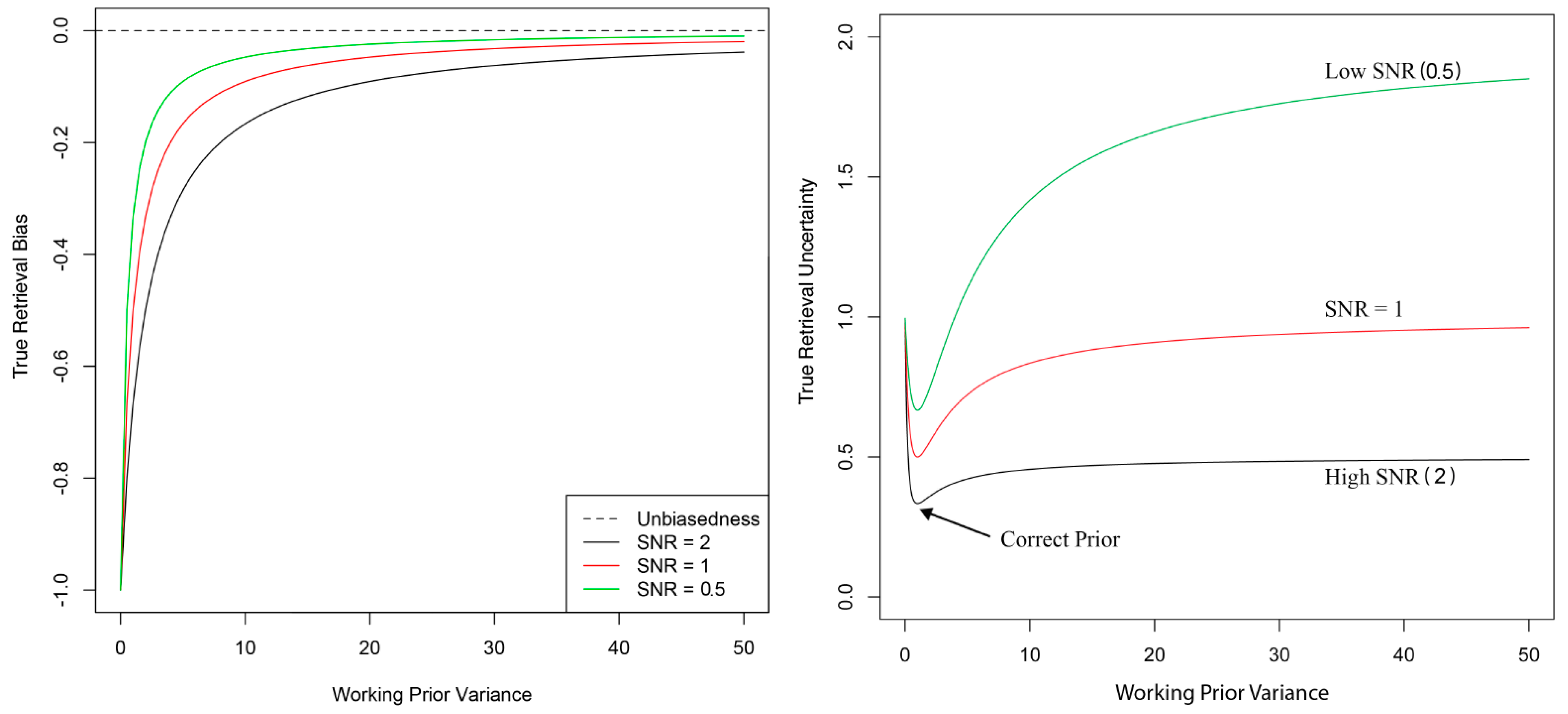
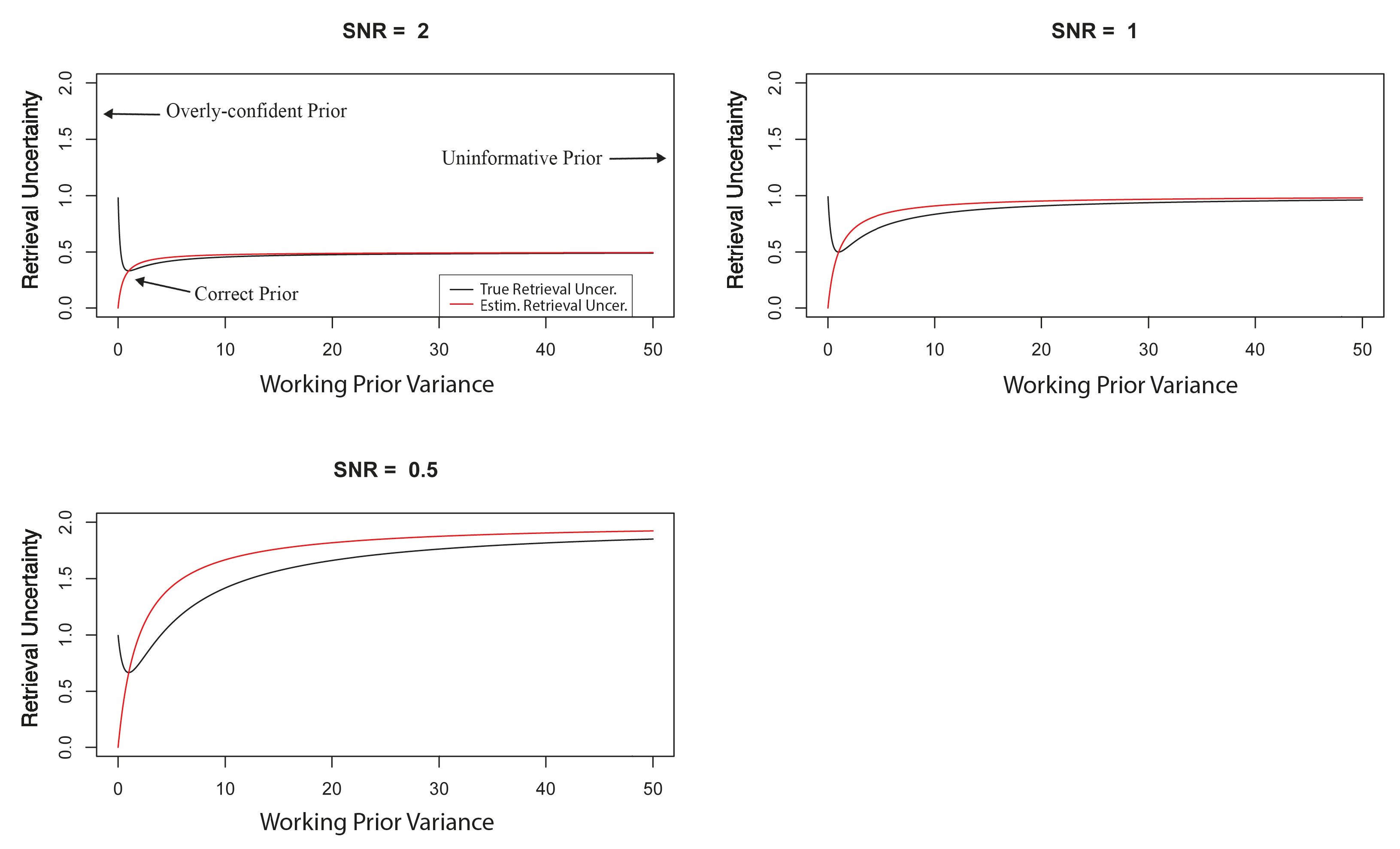
Section 2, we derive the multivariate equations for the bias and error variances arising from prior misspecification. We give a simple example of a univariate state, to gain intuition into the properties implied by the multivariate equations. We also give the multivariate bias vector and error covariance matrix for a particular choice of prior—the uninformative prior—versus the traditional prior used in OE retrievals, and we discuss the theoretical trade-offs between the choices therein. In Section 3, we design a simulation study using a surrogate OCO-2 linear forward model to evaluate empirically the consequences of prior misspecification, which we then compare to the theoretical derivations. This simulation study concretely demonstrates the trade-offs implied by the OCO-2 practice of inflating the working-prior covariance matrix. In Section 4, we conclude with some observations and practical recommendations on choosing a prior, for Optimal Estimation of the state from satellite remote sensing data.

2. Derivation of Retrieval Equations

The OE framework, as formalized in [1], can be viewed as a Bayesian approach to solve inverse problems in remote sensing. In this section, we review OE and derive the bias and error of an OE retrieval arising from misspecification of the prior.
In many OE applications, the forward model is nonlinear, and solving for the optimal solution requires iterative optimization methods such as the Levenberg–Marquardt algorithm (e.g., [20]). The nonlinear solver introduces complicating optimization-specific factors such as local minima, convergence criteria, linearization, and numerical stability. These can make it difficult to isolate the effect of prior misspecification within the resulting error analysis. Therefore, in this paper, we shall focus on the leading case of a linear forward model. Our derivations are in fact highly relevant to nonlinear problems, as this linearization approach is also used in quantifying the uncertainty of the OE retrieval ([1], Section 5.5). When the forward model is moderately or highly nonlinear, the conclusions derived from the linear case can be viewed as first-order approximations [1,21]. Our derivations in this section are general and relevant to any estimate based on OE, not just those used in remote sensing.

2.1. Background

Consider the case where an N-dimensional radiance vector y is related to the r-dimensional (hidden) true state x by the following data model:
y = F ( x ) + ϵ ,
where F ( · ) is the N-dimensional vector-valued forward model, x is the r-dimensional Gaussian true state with true mean x T and true covariance matrix S T , and ϵ is the N-dimensional Gaussian measurement-error vector with mean 0 and covariance matrix S ϵ , independent of x . That is, x Gau r ( x T , S T ) and ϵ Gau N ( 0 , S ϵ ) , where Gau n ( μ , Σ ) denotes an n-dimensional Gaussian (or normal) distribution with mean vector μ and covariance matrix Σ . For the leading case of a linear forward model, Equation (1) becomes
y = c + K x + ϵ ,
where the N × r matrix K = F x is the Jacobian of the forward model, and c is an N-dimensional constant vector. The linear model in Equation (2) could be thought of as the first-order term of the Taylor-series expansion of the nonlinear model (1) around some known state vector (e.g., [8]). Here, we assume that E ( ϵ ) = 0 and S ϵ is known.
Without loss of generality, we can assume that c = 0 (since c is known and hence in principle can be subtracted from y ), in which case y is a vector of “centered” radiances. Our data model then becomes
y = K x + ϵ .
Rodgers [1] proposes a loss function L ( · ) that is the negative logarithm of the posterior distribution of x given y ; that is, after dropping constant terms,
L ( x ) 2 log P ( x | y ) = ( y K x ) S ϵ 1 ( y K x ) + ( x x T ) S T 1 ( x x T ) .
The maximum a posteriori (MAP) solution (also the posterior mean in our case where the forward model is linear) is then given by
x ^ T = x T + G T ( y K x T ) ,
where G T is called the gain matrix and is given by G T = ( S T 1 + K S ϵ 1 K ) 1 K S ϵ 1 . The uncertainty on x ^ is then given by the error covariance matrix,
Σ T var T ( x ^ T x ) = ( S T 1 + K S ϵ 1 K ) 1 ,
where the subscript T on the variance operator indicates that statistical calculations are with respect to the true prior parameters { x T , S T } . The formulation above assumes that the prior mean vector and covariance matrix, { x T , S T } , are known perfectly. In practice, this is rarely the case. As discussed in Section 1, we draw a distinction between the (often unknown) true prior parameters { x T , S T } and the specified working prior parameters { x w , S w } , which are used in algorithms and are often constructed from a mixture of educated guesses, empirical studies, need for computational expediency, and subject-matter expertise. Since the distribution of the state is assumed Gaussian, we abuse notation slightly by referring to { x T , S T } as the true prior and { x w , S w } as the working prior. Researchers have long recognized that retrieval uncertainty in Equation (6) is incorrect when { x w , S w } { x T , S T } (e.g., [1,8,16,17,21]). To understand the effects of prior misspecification, we shall examine separately the effect on the retrieval bias (Section 2.2) and the effect on the retrieval uncertainty (Section 2.3). For ease of reference, we provide a list of the common mathematical symbols used in this paper and their meaning in Table 1.
We note that, in strictly Bayesian tradition, some might object to calling { x T , S T } the ‘true’ prior since the prior is popularly interpreted as an opinion or starting point. However, we shall show that for remote sensing problems where x Gau r ( x T , S T ) , the prior { x T , S T } is desirable in that it possesses properties such as unbiasedness (Section 2.2), efficiency (Section 2.5), and validity (Section 2.6), all of which are important for instrument design, validation, and scientific analysis. This explains why the existing literature recommends making { x w , S w } as close to { x T , S T } as possible (e.g., [1,16,17]). For this reason, we call { x T , S T } the ‘true’ prior.

2.2. Bias Arising from Prior Misspecification

Having specified the working prior { x w , S w } , the MAP estimate x ^ w is
x ^ w = x w + G w ( y K x w ) ,
where the subscript w on the the retrieved value x ^ w and the gain matrix G w indicates that they both depend on the working prior. The working gain matrix G w has the following form:
G w = ( S w 1 + K S ϵ 1 K ) 1 K S ϵ 1 .
When the working prior { x w , S w } is separated notationally from the true prior { x T , S T } , it is easy to calculate the working retrieval bias and the true retrieval bias from Equation (7) as a function of the working prior. We differentiate between the two calculations using the subscript ‘w’ and ‘T’, respectively. The working retrieval bias is simply
b w ( x w , S w ) E w ( x ^ w x ) , = E w ( x w + G w ( y K x w ) x ) , = x w 0 x w , = 0 ,
which we see below can give a false sense of security. In fact, the actual or true retrieval bias is
b T ( x w , S w ) E T ( x ^ w x ) , = E T ( x w + G w ( y K x w ) x ) , = ( I G w K ) ( x w x T ) , ( I A w ) ( x w x T ) ,
where A w G w K is the working averaging kernel. From (8), it is straightforward to show that ( I A w ) = ( S w 1 + K S ϵ 1 K ) 1 S w 1 , which when substituted into (9) gives
b T ( x w , S w ) = ( S w 1 + K S ϵ 1 K ) 1 S w 1 ( x w x T ) .
The key difference between the bias formula in Equation (10) and its treatment in Section 3.4.2 of [1] is that our result is general for any working prior { x w , S w } . From Equation (10), we see that the expected bias is equal to the product of the difference vector of prior means, ( x w x T ) , and the matrix ( S w 1 + K S ϵ 1 K ) 1 S w 1 . This result is significant because it indicates that, in a typical OE implementation, there is a non-zero bias equal to ( S w 1 + K S ϵ 1 K ) 1 S w 1 ( x w x T ) if the working-prior mean vector is not the same as the true-prior mean vector. In many applications, retrieval biases are highly undesirable, and significant efforts are devoted to preventing or removing them. Our results above indicate that an incorrect working-prior mean vector is a likely contributing source of bias in OE retrievals, and its role should be examined as part of the data-validation process, in addition to other potential causes such as calibration or spectroscopy. Fortunately, the result in Equation (10) also indicates that it is possible to reduce the magnitude of the bias by the choice of the working-prior covariance matrix, as we shall see below.
Assume that the working-prior covariance matrix S w is positive-definite; since K S ϵ 1 K is positive-semidefinite, then the matrix ( S w 1 + K S ϵ 1 K ) 1 S w 1 is positive-definite. Thus, the true retrieval bias b T ( x w , S w ) = 0 , if the working-prior mean vector is correct (i.e., x w = x T ). Clearly, x w = x T is a sufficient condition for unbiasedness. However, note that OE retrievals can be unbiased when the working-prior covariance matrix S w is incorrect, as long as the working-prior mean x w is correct.
Looking closely at Equation (10), we see that a bias term ( x w x T ) is multiplied by ( S w 1 + K S ϵ 1 K ) 1 S w 1 . Recall that S w is positive-definite and K S ϵ 1 K is positive-semidefinite; then, it is easy to show that 0 < ( S w 1 + K S ϵ 1 K ) 1 S w 1 I , where B A means that A B is positive-semidefinite, and B < A means that A B is positive-definite. Therefore, we can interpret this multiplicative term as ‘shrinking’ the bias depending on the relative strength between the working-prior covariance S w and the measurement-error contribution ( K S ϵ 1 K ) 1 . Mathematically, the latter matrix could be interpreted as the variance of the maximum-likelihood estimate of x using a frequentist approach (Section 2.6). Physically, it could also be interpreted as an expression of the measurement-error variability in the lower-dimensional state-space. When S w is much ‘smaller’ than ( K S ϵ 1 K ) 1 (that is, we have a lot of confidence and hence tight constraints on the trace or determinant of S w ), then ( S w 1 + K S ϵ 1 K ) 1 S w 1 ‘approaches’ I , and hence the bias ‘approaches’ ( x w x T ) . Another implication of Equation (10) is that we can greatly reduce the bias resulting from an incorrect working prior, by relaxing constraints and being overly conservative in choosing our working-prior covariance matrix S w . That is, if we let S w be unrealistically ‘large’ relative to ( K S ϵ 1 K ) 1 , then the bias ‘approaches’ 0 . More formally, let S w , which we define as min ( λ 1 ( S w ) , , λ r ( S w ) ) , with λ i ( S w ) being the i-th eigenvalue of S w . Then, ( S w 1 + K S ϵ 1 K ) 1 S w 1 0 , and
b T ( x w , S w ) b T ( x w , ) 0 .
The results in Equation (11) are noteworthy, since the choice, S w (equivalently, S w 1 0 ), constitutes a type of uninformative prior that is implicit in the frequentist maximum-likelihood formulation, a popular alternative choice for atmospheric retrievals ([22] e.g., the AIRS CO 2 retrieval algorithm). That is, the maximum-likelihood (also called least-squares) cost function is
L M L ( x ) = ( y K x ) S ϵ 1 ( y K x ) ,
which, in comparison to the OE cost function in Equation (4), can be seen as a limiting case where S w . For instance, Cressie et al. [18] showed that the AIRS least-squares retrieval can be considered to be an OE retrieval with an uninformative prior, in support of Equation (11).
In the rest of this paper, we shall use “OE” to refer to the case where estimates arise from an informative prior, and we shall use “least squares” or “maximum likelihood” to refer to the case of an uninformative prior. From Equation (11), we see that least-squares methods have an advantage over OE in that their retrievals are always unbiased, while OE retrievals with an informative prior are biased whenever the working-prior mean x w is misspecified. However, as seen in Section 2.5, least-squares-methods are statistically inefficient, often considerably so.
We note that, in many applications, researchers are interested in a linear combination of x ^ . In the case of OCO-2, for instance, the state vector x is convolved into the single value called total-column carbon dioxide (XCO2) using a linear pressure weighting vector h ; that is, XCO 2 = h x . Then, the bias in XCO2 is
b T ( x w , S w ) = E ( h x ^ h x ) = h E ( x ^ x ) = h b T ( x w , S w ) ,
where the expression for b T ( x w , S w ) is given in Equation (10). We note that most of the conclusions in this section will hold in the scalar XCO2 space, although the XCO2 bias will vary in magnitude depending on the L2-algorithm team’s choice of the pressure weighting vector h . In theory, it is possible for the XCO2 bias to be 0 if h is orthogonal to the bias vector b T ( x w , S w ) . In practice, however, the pressure weighting function is constructed from physical motivations (e.g., [23]), independent of the misspecification between { x w , S w } and { x T , S T } . Consequently, it would be unwise to rely on h being orthogonal to b T ( x w , S w ) in order to remove bias.
In summary, we can conclude that the choice of working-prior mean vector x w is very important when OE is used to retrieve the state x , with a bias arising when the working-prior mean vector differs from the true-prior mean vector. The magnitude of this bias vector varies between | | ( x w x T ) | | and 0, depending on the working-prior covariance matrix S w . For algorithms using a working prior where S w , the bias b T approaches 0 regardless of the choice of the working-prior mean vector x w .

2.3. Inaccurate Uncertainty Arising from Prior Misspecification

In the previous section, we saw that, for OE, a misspecified prior-mean vector x w results in a biased retrieval. We now consider the effect of misspecification of the prior on the retrieval uncertainty (i.e., the retrieval-error covariance matrix). From the working prior, the OE algorithm produces its own internal estimate of the retrieval uncertainty, Σ w ( x w , S w ) , as follows:
Σ w ( x w , S w ) var w ( x ^ w x ) = ( S w 1 + K S ϵ 1 K ) 1 ,
where the subscript w on Σ w ( · ) is consistent notation that indicates it is calculated with respect to the working prior. It is seen later in this subsection that the quantity Equation (13) can be equal to var T ( x ^ w x ) given by Equation (15), provided S w is the same as the true-prior covariance matrix S T . Rodgers [1] recognized that this condition is very restrictive and one that is unlikely to be achieved in practice. Therefore, he recommended restraint and circumspection in the interpretation of Equation (13), noting that to “estimate [the retrieval uncertainty] correctly, the actual statistics of the fine structure must be known. It is not enough to simply use some ad hoc matrix that has been constructed as a reasonable a priori constraint in the retrieval. If that real covariance matrix is not available, it may be better to abandon the estimation of the smoothing error, and consider the retrieval as an estimate of the smoothed version of the state, rather than an estimate of the complete state.” ([1] Section 3.2.1).
Here, we make Rodgers’ warning mathematically precise, in addition to providing some guidance on choosing a ‘good’ prior. The true retrieval uncertainty is derived as follows:
Σ T ( x w , S w ) = var T ( x ^ w x ) = var T ( x w + G w ( y K x w ) x ) = var T ( ( G w K I ) x + G w ϵ ) = ( G w K I ) S T ( G w K I ) + G w S ϵ G w
since x and ϵ are statistically independent, and recall from Equation (8) that G w = ( S w 1 + K S ϵ 1 K ) 1 K S ϵ 1 . Substituting this into Equation (14), we see that
Σ T ( x w , S w ) = ( S w 1 + K S ϵ 1 K ) 1 ( S w 1 S T S w 1 + K S ϵ 1 K ) ( S w 1 + K S ϵ 1 K ) 1 .
We note here that both the working retrieval uncertainty and the true retrieval uncertainty in Equations (13) and (15), respectively, are dependent only on S w and S T . This means that the accuracy of var w ( x ^ w x ) is not affected by misspecification of the prior-mean vector x w . Now, in practice, the mean-squared error (MSE) is an alternative measure of validation performance. It is the sum of the ‘squared’ retrieval bias and the true retrieval uncertainty as given by
M S E E T ( ( x ^ w x T ) ( x ^ w x T ) ) = b T ( x w , S w ) b T ( x w , S w ) + Σ T ( x w , S w ) .
Hence, the retrieval MSE is affected by both misspecifications, x w x T and S w S T .
It is straightforward to show that, when S w = S T , Equations (13) and (15) are the same:
Σ T ( x T , S T ) = ( S T 1 + K S ϵ 1 K ) 1 ( S T 1 S T S T 1 + K S ϵ 1 K ) ( S T 1 + K S ϵ 1 K ) 1 = ( S T 1 + K S ϵ 1 K ) 1 = Σ w ( x w , S w ) ,
since S w = S T . When S w S T , we show in Section 2.5 that Σ T ( x w , S w ) is ‘larger’ than Σ T ( x T , S T ) , and hence ( x ^ T x ) has smaller variability than ( x ^ w x ) .
The results in Equations (13) and (15) indicate that there is a difference between the true uncertainty Σ T ( x w , S w ) and the working uncertainty Σ w ( x w , S w ) when S w S T . This is important for OE products whose uncertainties are used downstream in later scientific analyses. For instance, the OCO-2 data are often used in CO 2 flux inversion, where the working uncertainties Σ w ( x w , S w ) , or linear combinations thereof, are often assumed to be equal to the true uncertainties Σ T ( x w , S w ) . Therefore, having inaccurate Σ w ( x w , S w ) in XCO2 retrievals may have adverse consequences in subsequent CO 2 -flux-inversion studies (e.g., [14]).
To gain some intuition into the bias and uncertainty under prior misspecification, in the next subsection, we consider a univariate state (i.e., r = 1 ). This allows us to demonstrate some interesting theoretical trade-offs between two particular classes of priors. Then, the general case of a multivariate state vector r is presented in Section 2.5 and Section 2.6.

2.4. Univariate Case Study

To understand further the behavior of the true bias and true uncertainty of the retrieval, we consider a simple univariate forward model, which we use to help interpret the multivariate formulas given by Equations (10) and (15). In this subsection, we assume that both the radiance y and the state x are scalars and that the data model is
y = k x + ϵ ,
where x Gau ( x T , σ T 2 ) and ϵ Gau ( 0 , σ ϵ 2 ) independently, and k , x T , σ T 2 , and σ ϵ 2 are one-dimensional versions of the terms K , x T , S T , and S ϵ , respectively. The OE retrieval and its uncertainty can be obtained as a special case of Equations (5) and (6). Then, the true retrieval bias (10) becomes
b T ( x w , σ w 2 ) = 1 σ w 2 + k 2 σ ϵ 2 1 1 σ w 2 ( x w x T ) .
In what follows, we pay particular attention to the state-space signal-to-noise ratio (SNR), which is the ratio of the variability of the signal ( σ T 2 ) to the measurement-error variability expressed in the state space ( σ ϵ 2 / k 2 ) . Note that, in the remote sensing literature, SNR is typically computed within radiance space; it is usually defined as the ratio of the reference radiance intensity to the standard deviation of the radiance noise ϵ . To make it clear that our SNR refers to the state space, we shall refer to the ratio σ T 2 ( σ ϵ 2 / k 2 ) as the state-space SNR. To see the effects on the true retrieval bias Equation (18), we consider three cases of state-space SNR: 0.5, 1, and 2. We fix the parameters k = 1 , x w = 0 , x T = 1 , and σ T 2 = 1 , and, consequently, the three cases correspond to σ ϵ 2 { 0.5 , 1 , 2 } .
The bias b T , as a function of the working-prior variance σ w 2 , is plotted in the left panel of Figure 1. It is clear that the bias is negative and largest when unquestioning confidence ( σ w 2 = 0 ) is put on the incorrect prior mean x w = 0 ; recall that the true prior mean is x T = 1 . In this case, the bias is simply x w x T = 1 . As σ w 2 increases from 0, the bias decreases monotonically towards 0. The rate at which the bias is reduced depends on the state-space SNR. The case of SNR = 2 shows a bias decreasing to 0 faster than the case of SNR = 1, which decreases to 0 faster than the case of SNR = 0.5.
Assume that the univariate retrieval model given by Equation (17); then, by substituting r = 1 into Equation (15), we obtain the univariate true retrieval-error variance:
s T 2 ( x w , σ w 2 ) = 1 σ w 2 + k 2 σ ϵ 2 1 1 σ w 4 σ T 2 + k 2 σ ϵ 2 1 σ w 2 + k 2 σ ϵ 2 1 ,
which is plotted in the right panel of Figure 1 as a function of σ w 2 , for SNR { 0.5 , 1 , 2 } . We see that, for all three SNRs, the true uncertainty s T 2 is smallest when the working-prior variance σ w 2 is equal to the true-prior variance σ T 2 = 1 . That is, s T 2 ( x T , σ T 2 ) s T 2 ( x w , σ w 2 ) for all { x w , σ w 2 } . This inequality demonstrates the statistical efficiency (i.e., smallest uncertainty) of the retrieval when using the true prior; it is easy to show that statistical efficiency holds for σ w 2 = σ T 2 and all choices of { k , x w , σ ϵ 2 , x T , σ T 2 } . In Section 2.5, we prove the result in the multivariate context where the state dimension r 2 .
In Section 2.2, we saw that the uninformative working prior (i.e., σ w 2 ) that is implicit in least-squares methods has the advantage of yielding unbiased estimates (Figure 1, left panel). However, the right panel of Figure 1 indicates that an uninformative working prior (i.e., σ w 2 ) yields statistically inefficient retrievals, since σ w 2 has to be equal to σ T 2 = 1 to achieve statistical efficiency.
Another major conclusion we can draw from the right panel of Figure 1 is that the uninformative working prior results in a retrieval that is fairly close in performance to that of the true prior when the state-space SNR is high (here, the blue curve, where SNR = 2). This agrees well with intuition because, when SNR is high, there is more information in the data, and we can afford not to inject additional information in the form of a small working-prior variance σ w 2 . In contrast, when SNR is low (here, the green curve, where SNR = 0.5), an uninformative working prior does not work nearly as well; with less information in the data, a smaller working-prior variance σ w 2 is needed for a retrieval that has acceptable variability.
Thus far, we have discussed the behavior of the true retrieval-error variance as a function of the working-prior variance. We now compare the true retrieval-error variance s T 2 ( x w , σ w 2 ) and the working retrieval-error variance s w 2 ( x w , σ w 2 ) , obtained from the retrieval algorithm. Assume the univariate retrieval model given by (17); then, by substituting r = 1 into (13), we obtain the univariate working retrieval-error variance:
s w 2 ( x w , σ w 2 ) = 1 σ w 2 + k 2 σ ϵ 2 1 .
In Figure 2, we plot Equations (19) and (20) in three panels for the three choices of state-space SNRs, namely SNR { 0.5 , 1 , 2 } . One conclusion we can draw is that the working retrieval uncertainty (red line) can either underestimate or overestimate the true retrieval uncertainty (black line), depending on whether σ w 2 > σ T 2 or σ w 2 < σ T 2 , and the only two instances where they are the same are when σ w 2 = σ T 2 or when σ w 2 (uninformative working prior). Consequently, the OE retrieval uncertainty estimate is only statistically valid when the working-prior variance σ w 2 is correct ( σ w 2 = σ T 2 ) or when it is uninformative. Figure 2 also succinctly illustrates the trade-off between OE and least squares; least squares ( σ w 2 ) has the advantage of uncertainty estimates always being valid (discussed further in Section 2.6), though at the cost of the retrievals not being statistically efficient (i.e., the uncertainty is greater than the minimum shown for the black line in each of the three panels). This makes sense intuitively, since OE uses information from both the data and the prior, while least squares only uses information from the data. Assuming that the working-prior variance is correct, then OE is clearly more efficient than least squares due to its having the extra component of prior information. Since least squares is completely insulated from any potentially incorrect assumption about the prior (both mean and variance), its uncertainty estimates are always valid.
We now return to the fully general multivariate retrieval and its uncertainty. The next two subsections address efficiency and uncertainty validity of OE retrievals in the multivariate case.

2.5. Efficiency of OE under the True Prior

Generalizing from the univariate case, we wish to show that the OE retrieval under the true prior, where { x w , S w } = { x T , S T } , has the ‘smallest’ true retrieval uncertainty for all possible choices of { x w , S w } . That is, we wish to show that Σ T ( x T , S T ) Σ T ( x w , S w ) , for all x w and S w . From Equations (13) and (15), this efficiency result is equivalent to the following proposition:
Proposition 1.
Under the definitions given in Section 2.1,
( S T 1 + K S ϵ 1 K ) 1 ( S w 1 + K S ϵ 1 K ) 1 ( S w 1 S T S w 1 + K S ϵ 1 K ) ( S w 1 + K S ϵ 1 K ) 1 .
Proof. 
See Appendix A.  □
This result indicates that Σ T ( x T , S T ) is the ‘smallest variance’ possible for all estimators arising from the cost function given by Equation (4), and hence we say that the OE retrieval is efficient under the true prior and is generally inefficient under any working prior for which S w S T . Proposition 1 holds regardless of whether a Bayesian approach or a Twomey–Tikhonov approach is used to choose S w .
We note that, in many applications, the state vector x is converted to a different geophysical quantity through a linear combination. For instance, the OCO-2 instrument retrieves a 55-dimensional (53-dimensional for ocean observations) state vector that consists of a 20-level CO 2 profile, surface air pressure, surface albedos, aerosol profile, temperature scaling, humidity scaling, wavelength offset and scaling, fluorescence (land-only), wind speed (ocean only), and empirical orthogonal function (EOF) scale factors [2]. In practice, researchers are interested in the total-column carbon dioxide XCO 2 = h x , where h is the pressure weighting vector referred to in Section 2.2. Since the matrix inequality, Σ T ( x T , S T ) Σ T ( x w , S w ) , is defined as a Σ T ( x T , S T ) a a Σ T ( x w , S w ) a for all column vectors a , it follows that this efficiency proposition holds true for geophysical products that are linear combinations of the state vector x , such as XCO2 from the OCO-2 retrieval.
We have already noted that validation studies often use the mean squared error (MSE) as a measure of uncertainty. Recall from Section 2.3 that the MSE can be written as
M S E = b T ( x w , S w ) b T ( x w , S w ) + Σ T ( x w , S w ) .
Proposition 1 shows that the second term, Σ T ( x w , S w ) , is at a global minimum if S w = S T . In Section 2.2, we showed that, if x w = x T , the bias is equal to 0 , which implies that the first term is at a global minimum when x w = x T . Combining the two results, we see that the MSE is at a global minimum when { x w , S w } = { x T , S T } that is when the working prior is equal to the true prior.
Clearly, one of the advantages of the OE estimator with an informative prior is the potential to have the best of both worlds. That is, from Equations (16) and (21), we see that, when an OE algorithm uses the correct prior covariance matrix, its retrievals are statistically efficient, and its retrieval uncertainties are valid (validity is discussed below in Section 2.6). However, we note that this is by no means guaranteed, as indicated in Figure 2 where it is seen that using a ‘bad’ working prior (e.g., using an overly ‘large’ prior when the state-space SNR is low) results in the worst of both worlds, namely OE retrievals that are inefficient with retrieval uncertainties that are not valid. To avoid this, we give some recommendations in Section 4 on how to design a working prior based on these theoretical results.

2.6. Validity of the OE Retrieval Uncertainties

We have seen in the univariate case that, when the working-prior variance σ w 2 approaches infinity, the working retrieval uncertainty approaches the true retrieval uncertainty. In the multivariate case, this property is equivalent to Σ T ( x w , S w ) Σ w ( x w , S w ) when S w (i.e., the uninformative prior). Unfortunately, using this uninformative prior does not take into account any knowledge one might have about the true prior covariance matrix S T , resulting in a retrieval that is inefficient (Section 2.5).
We define validity of retrieval uncertainty as:
Σ w ( x w , S w ) = Σ T ( x w , S w ) ,
which we now discuss for OE. Cressie et al. [18] proved this validity property for S w and applied it to the AIRS CO 2 retrieval algorithm. For completeness, we sketch the proof below using the notation summarized in Table 1. Let S w in Equation (15); then,
Σ T ( x w , S w ) ( 0 + K S ϵ 1 K ) 1 ( 0 · S T + K S ϵ 1 K ) ( 0 + K S ϵ 1 K ) 1 = ( K S ϵ 1 K ) 1 ,
where we note that a pseudoinverse is used in Equation (22) when necessary [19]. Similarly, let S w in (13); then,
Σ w ( x w , S w ) ( 0 + K S ϵ 1 K ) 1 = ( K S ϵ 1 K ) 1 ,
which is identical to Equation (22). That is, using an uninformative working prior always produces valid retrieval uncertainties, which is the result given in [18]. Contrast this with OE retrievals where an informative working prior is used, which has the potential for efficiency and validity (but may result in neither). The uninformative prior gives up efficiency in exchange for guaranteed validity.
In principle, then, an OE practitioner could try to leverage some of the properties that result from using an uninformative prior by intentionally making S w ‘larger’ than the best current understanding of S T . This is precisely what happens in many OE applications where some components of the prior covariance matrix are assigned unrealistically large values, such as the CO 2 components of the prior covariance matrix in OCO-2’s XCO2 retrieval [11]. According to the theory developed in this section, such a strategy trades off a marginal decrease in efficiency of the retrieval for a marginal increase in validity of the retrieval uncertainty. Hence, when designing a working-prior covariance matrix S w , this trade-off should be guided by the state-space signal-to-noise ratio, which can be obtained by comparing the state-space measurement-error variability, ( K S ϵ 1 K ) 1 , to the science team’s intuitive understanding of S T .
As has already been noted, in some applications, ( K S ϵ 1 K ) is singular. In this situation, an alternative approach would be to project ( K S ϵ 1 K ) down to an invertible subspace, compute the inverse, and then project back. Ramanathan et al. [19] showed that this approach is equivalent to the Singular Value Decomposition retrieval, so that the term ( K S ϵ 1 K ) 1 becomes ( K S ϵ 1 K ) + , where + denotes the Moore–Penrose inverse. That is, a pseudoinverse of ( K S ϵ 1 K ) should be used if ( K S ϵ 1 K ) is singular or close to it. More discussion and recommendations are given in Section 4.

3. Simulated Data Using True Priors and CO 2 Retrievals Using Misspecified Priors

Having explored the theoretical implications of prior misspecification in Section 2, in this section, we demonstrate the consequences of prior misspecification in a simulation using data from an Observing System Simulation Experiment (OSSE) for CO 2 retrievals with a linearized, streamlined version of the OCO-2 forward model (also called a surrogate model; see [9]). The OCO-2 satellite was launched by NASA in July 2014 with the goal of providing high-resolution estimates of total-column carbon dioxide (XCO2). It is a near-infrared (IR) instrument measuring reflected solar radiation in three IR bands, resulting in a radiance vector of dimension N = 3048 .
In our simulation, we make use of the OCO-2 surrogate model in [9], which “makes some simplification for interpretability and computational efficiency while attempting to maintain the key components of the state vector and RT [radiative transfer] that contribute substantially to uncertainty in [total-column CO 2 ].” The surrogate model has N = 3048 and r = 39 ; that is, x is a 39-dimensional state vector consisting of a 20-level CO 2 profile, surface air pressure, surface albedo, and aerosol profiles. For an overview of the surrogate model and its parameterization of the state vector, see Section 3 of [9].
In this OSSE, we first designated a known distribution as the true prior, and we repeatedly sampled 1000 times the true state x from this true prior distribution. Here, the true prior, { x T , S T } that we used is the sample mean and sample covariance of 5000 retrieved states obtained after simulation from a nonlinear control case ([9], Section 4.3). Each true state x from the OSSE was then put into a linearized version of the surrogate forward model to produce a noise-free radiance vector. Then, a vector of radiance measurement error was sampled and added to the noise-free vector to produce the noisy radiance data vector y . Finally, from y , we obtained the retrieved state vector, x ^ w , using a working prior distribution; see (7).
The linearized version of the surrogate forward model in [9] is obtained as follows: We put F ( x ) = c + K x , where K is a Jacobian matrix chosen from one of the 5000 retrievals from the control case in [9], and c = F ( x T ) K x T . Because the forward model here is the same over all 1000 samples in the OSSE, and it is linear; this simulation exercise can be considered an OSSE ‘simplification’ of the atmosphere.
Hence, the OSSE produces 1000 true states x , 1000 corresponding noisy radiance data vectors y , and 1000 corresponding retrieved states x ^ w . The working prior { x w , S w } that we use to obtain x ^ w is based on the operational prior for OCO-2, which depends on latitude and time of the OCO-2 sounding and on a climatology obtained from the GLOBALVIEW dataset. We chose one such in the OSSE; see the Supplementary Materials. Interested readers can find the priors { x T , S T } and { x w , S w } , the pressure-weighting vector h , the Jacobian K , and the measurement-error matrix S ϵ in the Supplementary Materials.
In Table 2, we show the values of the true-prior mean and working-prior mean for all 39 state elements. The standardized difference, defined by the element-wise difference of the working-prior mean minus the true-prior mean divided by the square root of the true-prior variance, is displayed in the last column. The CO 2 elements here represent CO 2 mole-fraction concentrations at 20 different pressure levels in the atmosphere, though recall that these values are linearly combined into the scalar value called total-column carbon dioxide (XCO2) using a pressure weighting vector h . Here, the difference in XCO2 between the working-prior mean and the true-prior mean (computed as h · ( x w x T ) ) is 3.23 ppm. The standardized differences indicate that the means for the CO 2 block are mostly similar, but the means for the Lambertian mean albedos for the Strong CO 2 , Weak CO 2 , and O 2 A bands include some very large misspecifications. These choices are deliberate, since we wish to demonstrate the ability of a ‘large’ S w to mitigate a potentially large bias.
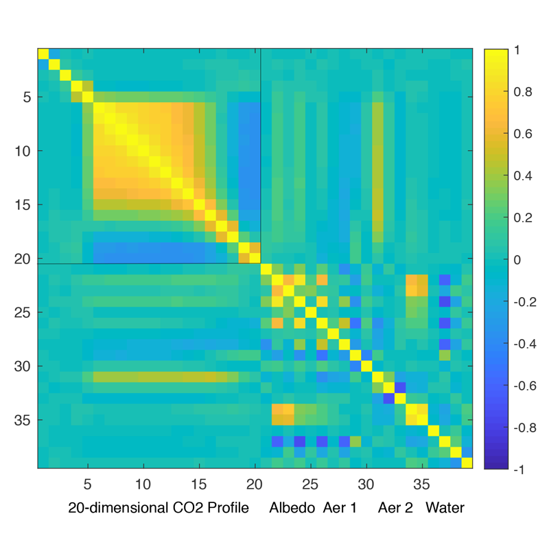
The OCO-2 working-prior covariance matrix S w is assumed to be diagonal for all non-CO 2 
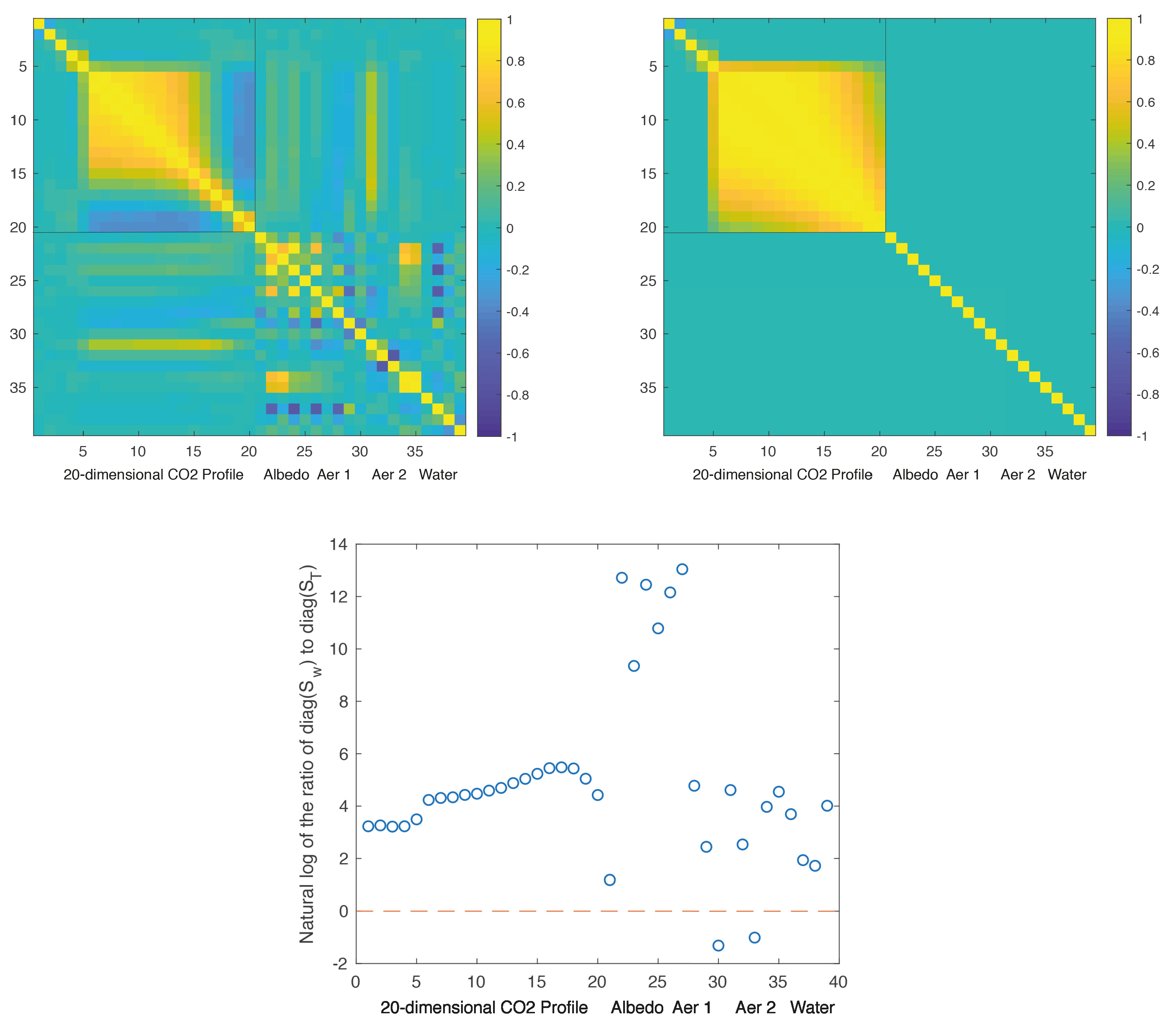
elements. To see how different the true-prior and working-prior covariances are, we show their correlation plots in Figure 3. Note that S T , unlike S w , has dependence between the aerosol, surface albedo, and water elements. We’ve chosen to show both of these plots in correlation space because these matrices in the original covariance space have vastly different magnitudes for almost all elements of the state vector. For instance, the CO 2 variance at Earth’s surface in the true prior is (5.22 ppm) 2 , while the corresponding CO 2 variance at Earth’s surface in the working prior is (47.7 ppm) 2 . In the bottom row of Figure 3, we illustrate the relative sizes of the diagonals of S w and S T (i.e., the prior variances) by plotting (on the log scale) their element-wise ratio at each of the 39 state elements. It is evident that, for our particular choice of S T , the diagonal elements of S w are larger by several orders of magnitude for most of the 39 elements, with the Lambertian Albedo elements (indices 22–27) being particularly large relative to the corresponding components in the true-prior covariance matrix. The only two exceptions to this are Dust Log Profile Thickness and Sea Salt Log Profile Thickness (indices 30 and 33, respectively). The OCO-2 operational algorithm imposes small prior variances for these elements because the forward model has minimal sensitivity to them [2,24].
This decision to inflate most components of S w by several orders of magnitude moves the working prior towards an uninformative prior (see Section 2.6), so that the working retrieval uncertainty should have better validity, although at the expense of statistical efficiency of the retrieval. The uninformative nature of the working-prior covariance matrix is noted in the development of the OCO-2 retrieval algorithm [11,20,23].
To see the different influences of the working-prior mean vector and the working-prior covariance matrix on the retrieval, the simulation experiment is divided into three parts, where we misspecify only the prior mean vector (Experiment 1: working prior = { x w , S T } ), where we misspecify only the prior covariance matrix (Experiment 2: working prior = { x T , S w } ), and where we misspecify both (Experiment 3: working prior = { x w , S w } ). The steps for our simulation experiments are as follows:
0.
Select a working prior from one of the three possibilities.
1.
Sample a state x from the true prior distribution { x T , S T } .
2.
Compute the radiance y using the model given by Equation (3).
3.
With the selected working prior, compute the retrieved XCO2 and the retrieval uncertainty (specifically, h x ^ w and h Σ w ( x w , S w ) h ) using Equations (7) and (13), respectively.
4.
Repeat steps 1–3 for 1000 iterations.
The summary statistics of the differences between the retrieved XCO2 and the true XCO2 under the three experiments are shown in Table 3. In Experiment 1, where only the prior mean is misspecified, the retrieval bias obtained from the simulation is 22.04 ppm! Table 3 shows that this agrees with a calculation based on the theoretical value given by Equation (10). This large retrieval bias is somewhat counter-intuitive, given that the misspecification of the prior mean of XCO2 (that is, h · ( x w x T ) ) is only 3.23 ppm. However, we note that the working prior mean also includes surface pressure, aerosols, and albedo, and, in this instance, the misspecification of these non-CO 2 elements has pushed the retrieval bias above 22 ppm. Some sensitivity analysis showed that a large part of this discrepancy is due to the mean albedo components used for the Strong CO 2 , Weak CO 2 , and O 2 A bands, which, in the OSSE, were deliberately misspecified as indicated by the SDiff column in Table 2.
Since there are 1000 simulated retrievals for each experiment, we could estimate a 95% confidence interval for the retrieval bias. We chose to use a nonparametric bootstrap based on 500 samples to do this [25]. In Experiment 1, we misspecified only the prior mean vector, and the simulation gave a retrieval bias of 22.04 ppm. As can be seen from Table 3, the empirical 95% confidence interval (CI) for the retrieval bias in Experiment 1 is [22.02 ppm, 22.06 ppm], which is consistent with the true retrieval bias of 22.04 ppm calculated from Equation (10). In Experiment 1 (and Experiment 3), the prior-mean vector was misspecified and the working bias of 0 is outside the 95% CI (and for Experiment 3). We also display the corresponding statistics for the retrieval uncertainty (in units of standard deviation) in the lower half of Table 3. In Experiment 1, where S w = S T , the analytical derivations show that the simulated retrieval uncertainty, the true retrieval uncertainty, and the working retrieval uncertainty should all be consistent with one another. From Table 3, we see that the true retrieval uncertainty is the same as the working retrieval uncertainty (0.31 ppm), both of which are consistent with the simulated retrieval uncertainty (0.30 ppm) and its 95% confidence interval.
In Experiment 2, we misspecified only the prior covariance matrix, and the simulation gave a retrieval bias of 0.02 ppm. As we noted in Section 2.2, x w = x T is a sufficient condition for unbiasedness, so the true retrieval bias under this experiment should be 0. Indeed, the 95% confidence interval of the bias for this experiment is [ 0.02 ppm, 0.05 ppm], which is consistent with the true value of 0. With regard to validity, the working retrieval uncertainty based on Equation (13) is 0.69 ppm, about 12% larger than the true retrieval uncertainty of 0.62 ppm based on Equation (15). The retrieval uncertainty from simulation is 0.61 and the 95% confidence interval is [0.58 ppm, 0.64 ppm], which is consistent with the true retrieval uncertainty of 0.62 ppm but not the working retrieval uncertainty of 0.69 ppm. This experiment reinforces our validity results in Section 2.3, namely that, when an informative prior covariance matrix is misspecified, the working retrieval uncertainty is incorrect.
In Experiment 3, we misspecified both the prior mean vector and the prior covariance matrix. From Table 3, the outcome is a mixture of Experiment 1 and Experiment 2, namely that the working retrieval has both a bias present and a retrieval uncertainty that is not valid. The trade-off between bias and variance is best captured in the square root of the MSE defined in Section 2.5 (or RMSE), which here is calculated from the simulation and is displayed in the last row of Table 3. The RMSE is largest (22.04 ppm) when the working-prior mean vector is incorrect, suggesting that in this experimental setup the RMSE is more sensitive to x w than to S w . However, when a conservative S w is applied, the same choice of x w has a much smaller RMSE, namely 0.72 ppm—see Table 3.
Experiment 3 provides a rationale behind the S w used in the operational OCO-2 prior. As was noted earlier in this Section, our choice of S w was modeled after the operational OCO-2 prior covariance matrix, where most elements are “unrealistically large for most of the world (all relatively clean-air sites), [in order to impose] a minimal constraint on the retrieved XCO2” [11]. In Experiment 1 where x w is misspecified but S w is not, the result is a bias of 22.04 ppm, but the same choice of x w and a misspecified, conservative S w in Experiment 3 results in a greatly mitigated bias of 0.41 ppm, about 50 times smaller than in Experiment 1! We repeated the experiments in this section with other choices of x w under varying degrees of misspecification, and we consistently obtained a reduction in the bias by multiplicative factors that ranged between 35 and 75. This implies that the operational OCO-2 retrieval, in its choice of working-prior covariance matrix, is quite robust to bias caused by using the wrong prior mean. We note that this attractive bias property comes with efficiency and validity trade-offs, which are discussed in Section 2.5 and Section 2.6.

4. Conclusions

In many remote sensing applications, the true priors are multivariate and hard to characterize properly, and a pragmatic approach is typically taken in designing the working prior { x w , S w } . This approach is a mixture of computational need for expediency, subject-matter expertise, and existing empirical data. In other words, the prior distributions within many OE application are typically constructed as a combination of the regularization approach (i.e., Twomey–Tikhonov constraint) and the Bayesian approach (i.e., distribution of the state). However, the retrieval uncertainties arising therefrom are almost universally interpreted within the Bayesian approach, often incorrectly. Here, our aim has been to show how this leads to biases and inaccuracies in OE retrievals and their uncertainties. We have done this by explicitly separating the true prior distribution, { x T , S T } , from the working prior distribution, { x w , S w } , and computing the true retrieval bias, E T ( x ^ w x ) , and the true retrieval uncertainty, var T ( x ^ w x ) . Our key findings can be summarized as follows:
  • When the prior mean is misspecified (i.e., x w x T ), there is a resulting bias that is given by ( S w 1 + K S ϵ 1 K ) 1 S w 1 ( x w x T ) . This bias can be reduced in magnitude by ‘increasing’ S w (that is, by making the working-prior covariance matrix less informative).
  • A corollary of the point above is that, when an instrument team observes a bias in their validation study, they should examine their choice of prior mean as a potential source of bias, in addition to other potential causes such as calibration or spectroscopy. If indeed the bias is caused by a misspecified prior mean, investigating only calibration or spectroscopy would be fruitless.
  • When the prior covariance is misspecified (i.e., S w S T , where S w 1 0 ), then the working retrieval uncertainty of the retrieval will not be valid with respect to the true retrieval uncertainty.
  • The limiting case, of making S w less and less informative, is S w 1 = 0 (equivalently S w ). This is the uninformative prior that is implicitly used in a least-squares (i.e., maximum-likelihood) approach. We show that the uninformative prior results in a retrieval uncertainty that has the attractive property of being valid (i.e., having an accurate working retrieval uncertainty) and unbiased. However, the OE framework with an informative working prior that is specified correctly has the advantage of being efficient (i.e., having the smallest possible retrieval-error variance, calculated using the true prior), valid, and a retrieval that is unbiased.
  • Importantly, with a ‘bad’ choice of prior, OE can have the worst of both worlds, being both not efficient and not valid. A compromise between the potential efficiency of OE and the guaranteed validity of least squares is obtained by erring on the ‘large’ side when setting the prior covariance matrix. This practice of inflating the prior covariance matrix to ‘relax’ constraints on the retrieval can be interpreted as trading some amount of efficiency for an increase in validity. Given the complicated settings, perhaps the best that the OE practitioner can hope for is an estimator that is ‘mostly’ efficient and ‘mostly’ valid.
  • The design of a working prior distribution should take into account the relative ‘size’ of the signal S T and the noise component ( K S ϵ 1 K ) 1 . The latter can be computed directly or as a pseudoinverse, and it should always be examined in order to have an idea of the contribution of the radiance noise in the state space. While the exact form of S T is typically not known, in practice, there are rough bounds available for the variability of each component of the state vector, and they can be compared to respective elements of ( K S ϵ 1 K ) 1 to obtain bounds on the state-space signal-to-noise ratio. If ( K S ϵ 1 K ) is singular, a Moore–Penrose pseudoinverse should be used instead.
  • When the signal components dominate (that is, when signal-to-noise ratios are larger than 1), then we could afford to use a less informative prior. If signal-to-noise ratios are much less than 1, then we recommend designing a more constrained prior with S w ‘more informative’ but hopefully close to S T .
In Section 3, we concretely demonstrated these findings in terms of XCO2 biases and RMSE on a linearized OCO-2 forward model. There, we showed that the OCO-2 team’s inflation of the working-prior covariance matrix essentially prioritizes validity over efficiency. As a consequence, the OCO-2 retrieval should be robust to biases arising from the choice of the working-prior mean vector, though at the cost of having sub-optimal retrieval uncertainties. It is important to note that inflating the working-prior covariance matrix in the OCO-2 retrieval algorithm does not guarantee unbiasedness, as it is still possible for the retrieval algorithm to be biased due to non-prior sources (e.g., spectroscopy, calibration, issues with the nonlinear optimization, etc.).
In this paper, we give an in-depth investigation of the bias and uncertainty of retrievals from Optimal Estimation (OE), when the prior distribution of the state is misspecified. Other misspecifications (which are not considered here) could be in the model for the observed radiances, namely misspecification of the measurement-error properties and/or of the radiative transfer function. In our case of a linear forward model, the latter manifests as a misspecification of the Jacobian. We also note that in this paper we have devoted considerable emphasis to XCO2 retrievals from OCO-2, but the theoretical results in Section 2 are fully general to OE retrievals, and hence they are applicable to any OE retrieval (e.g., SST from SEVIRI, temperature and ozone from TES, aerosols from MSG/SEVIRI, etc.).
In remote sensing applications, OE retrievals are sometimes compared to a different OE retrieval of the same process (e.g., XCO2 retrievals from the OCO-2 instrument and the TCCON instruments, retrieval assimilation in inversion studies, etc.). In this case, the two different retrievals are compared using an adjustment described by [26]. That is, given the retrievals x ^ 1 and x ^ 2 using priors { x 1 , S 1 } and { x 2 , S 2 } , respectively, an adjustment (also colloquially called “averaging kernel convolution”) is made to convert them to x ^ 1 C and x ^ 2 C by shifting them to a common “comparison ensemble” { x C , S C } [26].
A general misconception is that this averaging kernel convolution removes any bias introduced by prior misspecification (that is, E ( x ^ 1 C x ^ 2 C ) = 0 ). As an example of this misunderstanding, [27] noted, “the use of averaging kernels makes atmospheric inversion insensitive to the choice of a particular retrieval prior […] profile,” and provided a cite to [28], which is a theoretical precursor to the [26] paper discussed in this section. However, this statement by [27] is incorrect when the comparison ensemble is misspecified relative to the true variability of the state x . It is straightforward to show that E ( x ^ 1 C x ) 0 , E ( x ^ 2 C x ) 0 , and E ( x ^ 1 C x ^ 2 C ) 0 when { x C , S C } { x T , S T } . It is also straightforward to show, starting from the atmospheric inversion cost function, that the biases E ( x ^ 1 C x ) 0 and E ( x ^ 2 C x ) 0 will result in biased atmospheric inversions! In short, while the process of averaging kernel convolution described in [28] and [26] allows researchers and inversion modelers to shift their retrievals to a common prior { x C , S C } , the consequences of prior misspecification described in this paper still apply if { x C , S C } { x T , S T } .
Thus far, we have considered the impact of prior misspecification in the case of a linear forward model. Our results are directly applicable to linear or mostly linear retrievals (e.g., fluorescence; [29]). For many applications, the forward model is nonlinear, and the MAP solution is obtained using iterative least-squares methods such as the Levenberg–Marquardt algorithm (e.g., [11]). Estimates of the posterior uncertainty in this situation are difficult, mostly because there are two main complications with estimates of uncertainties based on iterative gradient methods. The first issue arises from complications in the optimization algorithm such as local minima, step-size, and convergence criteria. We are not aware of any analytical study on the effect of optimization parameters on the uncertainties for OE retrievals. Furthermore, note that current OE uncertainty estimates in remote sensing applications, which are based on [1], do not account for local minima or convergence criteria.
The second issue is that, even in the ideal case where there is no numerical problem (i.e., the algorithm always converges to the global minimum), it is difficult to compute estimates of uncertainties without having high-order derivatives, which are often computationally expensive to obtain [21]. The standard OE uncertainties in remote sensing applications, for instance, are computed by approximating the forward model with a first-order Taylor-series expansion around the global minimum x ^ and applying linear error analysis ([1], Section 5.5). Hence, OE uncertainty estimates for nonlinear problems (e.g., OCO-2 operational XCO2 uncertainties) are only valid for retrieved values for which (1) the gradient-descent algorithm has found the global minimum x ^ , and that (2) a first-order Taylor-series expansion is reasonable around x ^ given the instrument’s measurement errors (or, in [1]’s words, “[the Taylor-series expansion] about x [is] valid within ϵ in the moderately nonlinear case” ([1] p. 87). In the statistics research literature, Rodgers’ [1] approach is called the delta method. Similarly, our linear derivations and results extend straightforwardly via the delta method to nonlinear problems whenever the same two conditions (1) and (2) above apply.

Author Contributions

H.N. and N.C. developed the ideas and the statistical theory. H.N. performed the computations. J.H. carried out data curation and provided expertise on the forward model. All authors discussed the results. H.N. wrote the first draft, and all authors contributed to subsequent drafts.

Funding

H.N. and J.H.’s research was performed at the Jet Propulsion Laboratory, California Institute of Technology, under contract with NASA. N.C.’s research was performed under NASA ROSES NNH17ZDA001N and Australian Research Council Discovery Projects, DP150104576 and DP190100180.

Acknowledgments

The authors would like to thank Mike Turmon at the Jet Propulsion Laboratory for his insightful comments on the manuscript, and Rui Wang for initial discussions on prior misspecification. We are also grateful to the four referees for their careful reading of the manuscript and for their constructive comments.

Conflicts of Interest

The authors declare no conflict of interest.

Appendix A. Proof of Proposition 1

Proposition A1.
Under the definitions given in Section 2.1, Σ T ( x T , S T ) Σ T ( x w , S w ) for all x w and S w , or equivalently,
( S T 1 + K S ϵ 1 K ) 1 ( S w 1 + K S ϵ 1 K ) 1 ( S w 1 S T S w 1 + K S ϵ 1 K ) ( S w 1 + K S ϵ 1 K ) 1 .
Proof. 
The proof relies on the observation that this proposition is related to the Schur complement (e.g., [30]). For a symmetric matrix
X A B B C ,
where C is invertible, the Schur complement of C in X is defined as X / C A B C 1 B . The Schur-complement theorem states that, if C > 0 , then X 0 if and only if its Schur complement X / C 0 (e.g., [30], Theorem 1.12).
Now, consider the matrix,
E = S w 1 S T S w 1 + K S ϵ 1 K S w 1 + K S ϵ 1 K S w 1 + K S ϵ 1 K S T 1 + K S ϵ 1 K .
We can rewrite E as the sum of two symmetric matrices,
E = E 1 + E 2 ,
where
E 1 = S w 1 S T S w 1 S w 1 S w 1 S T 1 ,
and
E 2 = K S ϵ 1 K K S ϵ 1 K K S ϵ 1 K K S ϵ 1 K = K S ϵ 1 K 1 1 1 1 .
First, consider the term E 1 : we see that S T 1 > 0 , since S T is positive-definite, and that its Schur complement, E 1 / S T 1 = S w 1 S T S w 1 S w 1 S T S w 1 = 0 . Therefore, by the Schur-complement theorem, E 1 0 . Second, consider the term E 2 : from (A2), we see that E 2 is the Kronecker product of K S ϵ 1 K and the 2 × 2 matrix of all 1’s, both of which are positive-semidefinite. Since the Kronecker product of two positive-semidefinite matrices is also positive-semidefinite ([31], Section 10.2.1), then E 2 0 . Hence, E = E 1 + E 2 0 .
From (A1), given that ( S T 1 + K S ϵ 1 K ) > 0 and E 0 , then, by the Schur-complement theorem, E / ( S T 1 + K S ϵ 1 K ) 0 . Consequently,
0 E / ( S T 1 + K S ϵ 1 K ) , 0 ( S w 1 S T S w 1 + K S ϵ 1 K ) ( S w 1 + K S ϵ 1 K ) ( S T 1 + K S ϵ 1 K ) 1 ( S w 1 + K S ϵ 1 K ) ,
and hence
( S T 1 + K S ϵ 1 K ) 1 ( S w 1 + K S ϵ 1 K ) 1 ( S w 1 S T S w 1 + K S ϵ 1 K ) ( S w 1 + K S ϵ 1 K ) 1 .
That is,
Σ T ( x T , S T ) Σ T ( x w , S w ) for all { x w , S w } .
  □

References

  1. Rodgers, C.D. Inverse Methods for Atmospheric Sounding: Theory and Practice; World Scientific Press: Singapore, 2000. [Google Scholar]
  2. O’Dell, C.W.; Eldering, A.; Wennberg, P.O.; Crisp, D.; Gunson, M.R.; Fisher, B.; Frankenberg, C.; Kiel, M.; Lindqvist, H.; Mandrake, L.; et al. Improved Retrievals of Carbon Dioxide from the Orbiting Carbon Observatory-2 with the version 8 ACOS algorithm. Atmos. Meas. Tech. 2018, 11, 6539–6576. [Google Scholar] [CrossRef]
  3. Merchant, C.; Le Borgne, P.; Roquet, H.; Legendre, G. Extended optimal estimation techniques for sea surface temperature from the Spinning Enhanced Visible and Infra-Red Imager (SEVIRI). Remote Sens. Environ. 2013, 131, 287–297. [Google Scholar] [CrossRef]
  4. Yoshida, Y.; Kikuchi, N.; Morino, I.; Uchino, O.; Oshchepkov, S.; Bril, A.; Saeki, T.; Schutgens, N.; Toon, G.C.; Wunch, D.; et al. Improvement of the retrieval algorithm for GOSAT SWIR XCO2 and XCH4 and their validation using TCCON data. Atmos. Meas. Tech. 2013, 6, 1533–1547. [Google Scholar] [CrossRef]
  5. Bowman, K.W.; Rodgers, C.D.; Kulawik, S.S.; Worden, J.; Sarkissian, E.; Osterman, G.; Steck, T.; Lou, M.; Eldering, A.; Shephard, M.; et al. Tropospheric Emission Spectrometer: Retrieval method and error analysis. IEEE Trans. Geosci. Remote Sens. 2006, 44, 1297–1307. [Google Scholar] [CrossRef]
  6. Irion, F.; Kahn, B.; Schreier, M.; Fetzer, E.; Fishbein, E.; Fu, D.; Kalmus, P.; Wilson, R.; Wong, S.; Yue, Q. Single-footprint retrievals of temperature, water vapor and cloud properties from AIRS. Atmos. Meas. Tech. 2018, 11, 971–995. [Google Scholar] [CrossRef]
  7. Govaerts, Y.; Wagner, S.; Lattanzio, A.; Watts, P. Joint retrieval of surface reflectance and aerosol optical depth from MSG/SEVIRI observations with an optimal estimation approach: 1. Theory. J. Geophys. Res. Atmos. 2010, 115. [Google Scholar] [CrossRef]
  8. Cressie, N. Mission CO2ntrol: A Statistical Scientist’s Role in Remote Sensing of Atmospheric Carbon Dioxide (with discussion). J. Am. Stat. Assoc. 2018, 113, 152–168. [Google Scholar] [CrossRef]
  9. Hobbs, J.; Braverman, A.; Cressie, N.; Granat, R.; Gunson, M. Simulation-based uncertainty quantification for estimating atmospheric CO2 from satellite data. SIAM/ASA J. Uncertain. Quantif. 2017, 5, 956–985. [Google Scholar] [CrossRef]
  10. Wunch, D.; Wennberg, P.; Toon, G.; Connor, B.; Fisher, B.; Osterman, G.; Frankenberg, C.; Mandrake, L.; O’Dell, C.; Ahonen, P.; et al. A method for evaluating bias in global measurements of CO2 total columns from space. Atmos. Chem. Phys. 2011, 11, 12317–12337. [Google Scholar] [CrossRef]
  11. Boesch, H.; Brown, L.; Castano, R.; Christi, M.; Connor, B.; Crisp, D.; Eldering, A.; Fisher, B.; Frankenberg, C.; Gunson, M.; et al. Orbiting Carbon Observatory (OCO-2) Level 2 Full Physics Algorithm Theoretical Basis Document. Available online: https://docserver.gesdisc.eosdis.nasa.gov/public/project/OCO/OCO2_L2_ATBD.V8.pdf (accessed on 12 December 2017).
  12. Connor, B.; Bösch, H.; McDuffie, J.; Taylor, T.; Fu, D.; Frankenberg, C.; O’Dell, C.; Payne, V.H.; Gunson, M.; Pollock, R.; et al. Quantification of uncertainties in OCO-2 measurements of XCO2: Simulations and linear error analysis. Atmos. Meas. Tech. 2016, 9, 5227. [Google Scholar] [CrossRef]
  13. Osterman, G.B.; Eldering, A.; Mandrake, L.; O’Dell, C.; Wunch, D.; Wennberg, P.O.; Fisher, B.; Marchetti, Y. Orbiting Carbon Observatory (OCO-2) Warn Level, Bias Correction, and Lite File Product Description; Technical Report; Jet Propulsion Laboratory, California Institute of Technology: Pasadena, CA, USA, 2017. [Google Scholar]
  14. Engelen, R.J.; Denning, A.S.; Gurney, K.R. On error estimation in atmospheric CO2 inversions. J. Geophys. Res. Atmos. 2002, 107, ACL-10. [Google Scholar] [CrossRef]
  15. Luo, M.; Rinsland, C.; Rodgers, C.D.; Logan, J.; Worden, H.; Kulawik, S.S.; Eldering, A.; Goldman, A.; Shephard, M.; Gunson, M.; et al. Comparison of carbon monoxide measurements by TES and MOPITT: Influence of a priori data and instrument characteristics on nadir atmospheric species retrievals. J. Geophys. Res. Atmos. 2007, 112. [Google Scholar] [CrossRef]
  16. Kulawik, S.S.; Bowman, K.W.; Luo, M.; Rodgers, C.D.; Jourdain, L. Impact of nonlinearity on changing the a priori of trace gas profile estimates from the Tropospheric Emission Spectrometer (TES). Atmos. Chem. Phys. 2008, 8, 3081–3092. [Google Scholar] [CrossRef]
  17. Su, Z.; Yung, Y.L.; Shia, R.L.; Miller, C.E. Assessing accuracy and precision for space-based measurements of carbon dioxide: An associated statistical methodology revisited. Earth Space Sci. 2017, 4, 147–161. [Google Scholar] [CrossRef]
  18. Cressie, N.; Wang, R.; Maloney, B. The Atmospheric Infrared Sounder retrieval, revisited. IEEE Geosci. Remote Sens. Lett. 2017, 14, 1504–1507. [Google Scholar] [CrossRef]
  19. Ramanathan, A.K.; Nguyen, H.M.; Sun, X.; Mao, J.; Abshire, J.B.; Hobbs, J.M.; Braverman, A.J. A singular value decomposition framework for retrievals with vertical distribution information from greenhouse gas column absorption spectroscopy measurements. Atmos. Meas. Tech. 2018, 11, 4909–4928. [Google Scholar] [CrossRef]
  20. Connor, B.J.; Boesch, H.; Toon, G.; Sen, B.; Miller, C.; Crisp, D. Orbiting Carbon Observatory: Inverse method and prospective error analysis. J. Geophys. Res. Atmos. 2008, 113. [Google Scholar] [CrossRef]
  21. Cressie, N.; Wang, R.; Smyth, M.; Miller, C.E. Statistical bias and variance for the regularized inverse problem: Application to space-based atmospheric CO2 retrievals. J. Geophys. Res. Atmos. 2016, 121, 5526–5537. [Google Scholar] [CrossRef]
  22. Susskind, J.; Barnet, C.D.; Blaisdell, J.M. Retrieval of atmospheric and surface parameters from AIRS/AMSU/HSB data in the presence of clouds. IEEE Trans. Geosci. Remote Sens. 2003, 41, 390–409. [Google Scholar] [CrossRef]
  23. O’Dell, C.W.; Connor, B.; Bösch, H.; O’Brien, D.; Frankenberg, C.; Castano, R.; Christi, M.; Eldering, D.; Fisher, B.; Gunson, M.; et al. The ACOS CO2 retrieval algorithm Part 1: Description and validation against synthetic observations. Atmos. Meas. Tech. 2012, 5, 99–121. [Google Scholar] [CrossRef]
  24. Butz, A.; Hasekamp, O.P.; Frankenberg, C.; Aben, I. Retrievals of atmospheric CO2 from simulated space-borne measurements of backscattered near-infrared sunlight: Accounting for aerosol effects. Appl. Opt. 2009, 48, 3322–3336. [Google Scholar] [CrossRef]
  25. Efron, B. Nonparametric estimates of standard error: The jackknife, the bootstrap and other methods. Biometrika 1981, 68, 589–599. [Google Scholar] [CrossRef]
  26. Rodgers, C.D.; Connor, B.J. Intercomparison of remote sounding instruments. J. Geophys. Res. Atmos. 2003, 108. [Google Scholar] [CrossRef]
  27. Chevallier, F. On the statistical optimality of CO2 atmospheric inversions assimilating CO2 column retrievals. Atmos. Chem. Phys. 2015, 15, 11133–11145. [Google Scholar] [CrossRef]
  28. Connor, B.J.; Parrish, A.; Tsou, J.J.; McCormick, M.P. Error analysis for the ground-based microwave ozone measurements during STOIC. J. Geophys. Res. Atmos. 1995, 100, 9283–9291. [Google Scholar] [CrossRef]
  29. Sun, Y.; Frankenberg, C.; Jung, M.; Joiner, J.; Guanter, L.; Köhler, P.; Magney, T. Overview of Solar-Induced chlorophyll Fluorescence (SIF) from the Orbiting Carbon Observatory-2: Retrieval, cross-mission comparison, and global monitoring for GPP. Remote Sens. Environ. 2018, 209, 808–823. [Google Scholar] [CrossRef]
  30. Horn, R.A.; Zhang, F. Basic properties of the Schur complement. In The Schur Complement and Its Applications; Zhang, F., Ed.; Springer: Boston, MA, USA, 2005; pp. 17–46. [Google Scholar]
  31. Petersen, K.B.; Pedersen, M.S. The Matrix Cookbook. Tech. Univ. Den. 2008, 7, 510. [Google Scholar]
Figure 1. Left panel: True retrieval bias (vertical axis) resulting from OE as a function of σ w 2 (horizontal axis) for a univariate model where x w = 0 , x T = 1 , and σ T 2 = 1 , for three choices of state-space SNRs. Right panel: The true retrieval-error variance s T 2 (vertical axis) given by Equation (19) as a function of the working-prior variance σ w 2 (horizontal axis) for the same three choices of state-space SNR.
Remotesensing 11 02770 g001
Figure 2. Working retrieval-error variance s w 2 given by Equation (20) (red lines) and true retrieval-error variance s T 2 given by Equation (19) (black lines) as a function of the working-prior variance σ w 2 for three choices of state-space SNRs: 2 (top left), 1 (top right), and 0.5 (bottom left). In the univariate model, the true-prior variance is σ T 2 = 1 .
Remotesensing 11 02770 g002
Figure 3. Top row: Plots of the true-prior correlation matrix (left panel) and the working-prior correlation matrix (right panel) used in the OSSE simulation. Bottom row: Natural log of the element-wise ratio of the diagonals of S w to the diagonals of S T . The red dashed line indicates the dividing line at which the working-prior variance is equal to the true-prior variance.
Remotesensing 11 02770 g003
Table 1. Reference guide for mathematical symbols.
Symbol           Definition
y Observed N-dimensional vector of radiances
x True (hidden) r-dimensional vector of state elements
ϵ N-dimensional vector of radiance error
K Jacobian of the forward model
x T True-prior mean vector of the state vector x
x w Working-prior mean vector of the state vector x
x ^ T Retrieved state vector under the true prior
x ^ w Retrieved state vector under a working prior
S ϵ Covariance matrix for the radiance-measurement-error vector ϵ
S T True-prior covariance matrix of the state vector x
S w Working-prior covariance matrix of the state vector x
G T Gain matrix under the true prior
G w Gain matrix under the working prior
b T ( · ) True retrieval bias for OE estimates (as a function of the working prior)
b w ( · ) Working retrieval bias for OE estimates
Σ T ( · ) True retrieval uncertainty for OE estimates (as a function of the working prior)
Σ w ( · ) Working retrieval uncertainty from the OE algorithm
Table 2. True-prior means and working-prior means used in the simulation (first and second column). The standardized difference (SDiff) for each element is defined as the difference of the working-prior mean minus the true-prior mean, divided by the square root of the true-prior variance of that element (third column).
NameTrueWorkingSDiff
CO 2 Volume Mixing Ratio [Means in ppm]
Vertical Level 1 (Top of Atmosphere)389.7404388.9731−2.6829
Vertical Level 2395.3024392.9746−4.7299
Vertical Level 3398.1116394.7076−5.2564
Vertical Level 4399.1278396.0390−3.8981
Vertical Level 5 (Tropopause)398.0690397.1398−0.9599
Vertical Level 6396.4378398.35722.4179
Vertical Level 7396.0817398.49192.7922
Vertical Level 8395.7496398.46472.8952
Vertical Level 9395.2420398.43253.1810
Vertical Level 10394.7879398.39673.3577
Vertical Level 11393.5765398.35793.8944
Vertical Level 12392.4954398.31594.2996
Vertical Level 13391.1232398.27074.7768
Vertical Level 14390.0250398.21905.1063
Vertical Level 15389.1317398.15985.1538
Vertical Level 16388.8229398.09505.0912
Vertical Level 17389.8204398.02503.8831
Vertical Level 18391.4878397.95142.6177
Vertical Level 19397.4609397.87800.1217
Vertical Level 20 (Surface)401.3001397.8112−0.6676
Surface Pressure [hPa]998.741310021.4769
Lambertian Albedo [units of means are in the Suppl. Mat.]
Strong CO 2 Band Mean Albedo0.64960.1753−273.7585
Strong CO 2 Band Albedo Spectral Slope000.00
Weak CO 2 Band Mean Albedo0.67550.2560−212.0764
Weak CO 2 Band Albedo Spectral Slope000.00
O2 A-Band Mean Albedo0.51830.1827−146.3876
O2 A-Band Mean Albedo Spectral Slope000
Aerosols [units of means are in the Suppl. Mat.]
Dust Log Aerosol Optical Depth−2.4760−3.3178−4.5838
Dust Profile Height0.89820.90000.0301
Dust Log Profile Thickness−3.6365−2.99571.8230
Sea Salt Log Aerosol Optical Depth−3.8290−4.0140−0.9278
Sea Salt Profile Height0.74780.90002.7018
Sea Salt Log Profile Thickness−2.0716−2.9957−3.0608
Cloud Ice Log Aerosol Depth−2.8718−4.3820−6.1065
Cloud Ice Profile Height0.22080.30003.8450
Cloud Ice Log Profile Thickness−3.2129−3.2189−0.1704
Cloud Water Log Aerosol Depth−4.0925−4.3820−0.4233
Cloud Water Profile Height0.55310.75001.1633
Cloud Water Log Profile Thickness−2.3013−2.3026−0.0995
Table 3. Simulation summary statistics for XCO2. Both the bias and the uncertainty (here expressed as a standard deviation) have units of ppm. Estimates that are consistent with the corresponding confidence intervals are colored red. The true retrieval bias and true retrieval uncertainties are computed using the derivations in Section 2.
Experiment 1Experiment 2Experiment 3
Working prior { x w , S T } { x T , S w } { x w , S w }
Bias from simulation22.040.010.40
95% CI for bias[22.02, 22.06][ 0.02 , 0.05][0.36, 0.44]
True retrieval bias22.0400.41
Working retrieval bias000
Uncertainty from simulation0.300.610.60
95% CI for uncertainty[0.29, 0.31][0.58, 0.64][0.57, 0.63]
True retrieval uncertainty0.310.620.62
Working retrieval uncertainty0.310.690.69
RMSE from simulation22.040.610.72

