Sub-Annual Calving Front Migration, Area Change and Calving Rates from Swath Mode CryoSat-2 Altimetry, on Filchner-Ronne Ice Shelf, Antarctica

 , , , , and
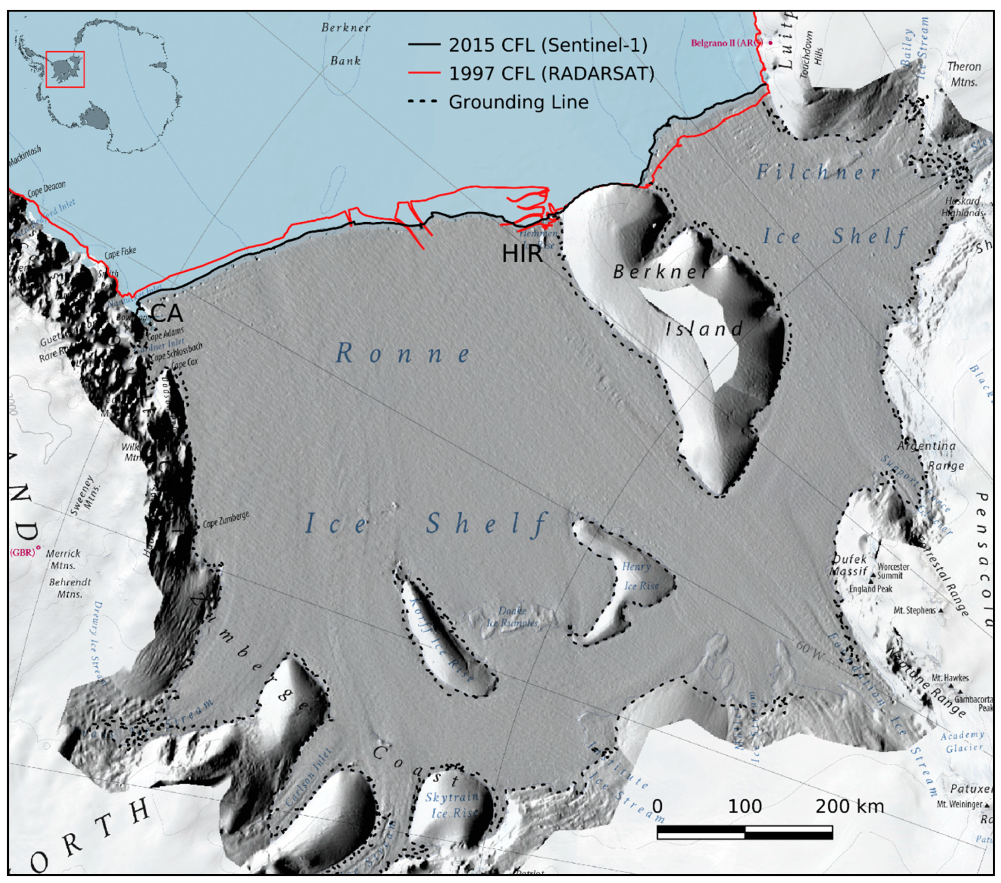
Abstract
1. Introduction
2. Study Region, Data and Methods
2.1. Study Region
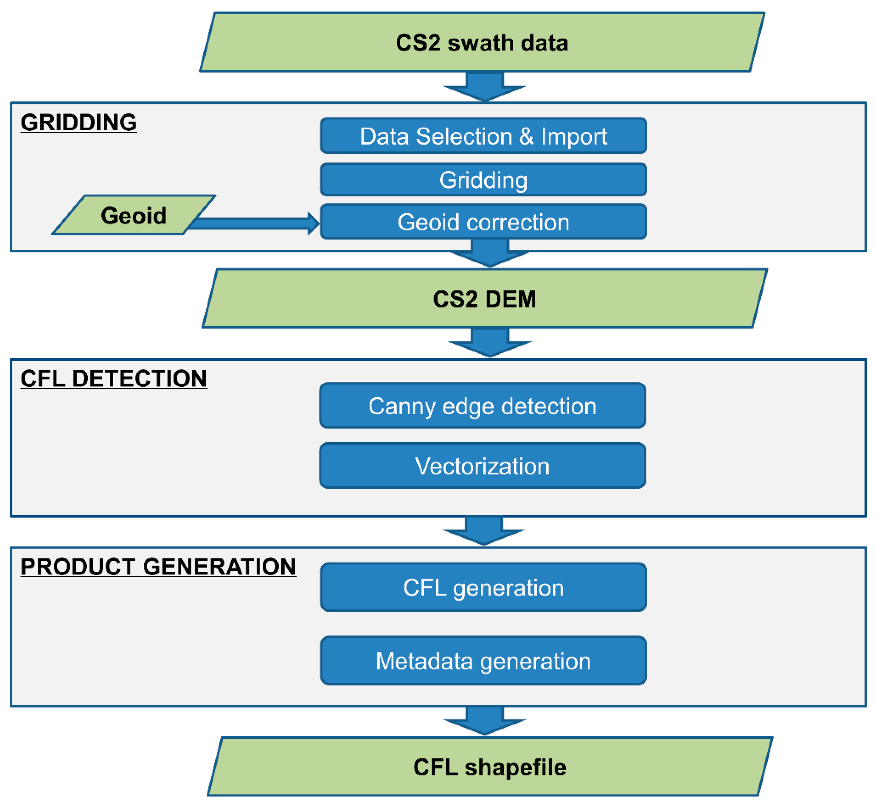
2.2. CryoSat-2 Data and Swath Mode Processing
2.3. Delineating the Calving Front
2.4. Area Change and Iceberg Calving Rate
3. Results
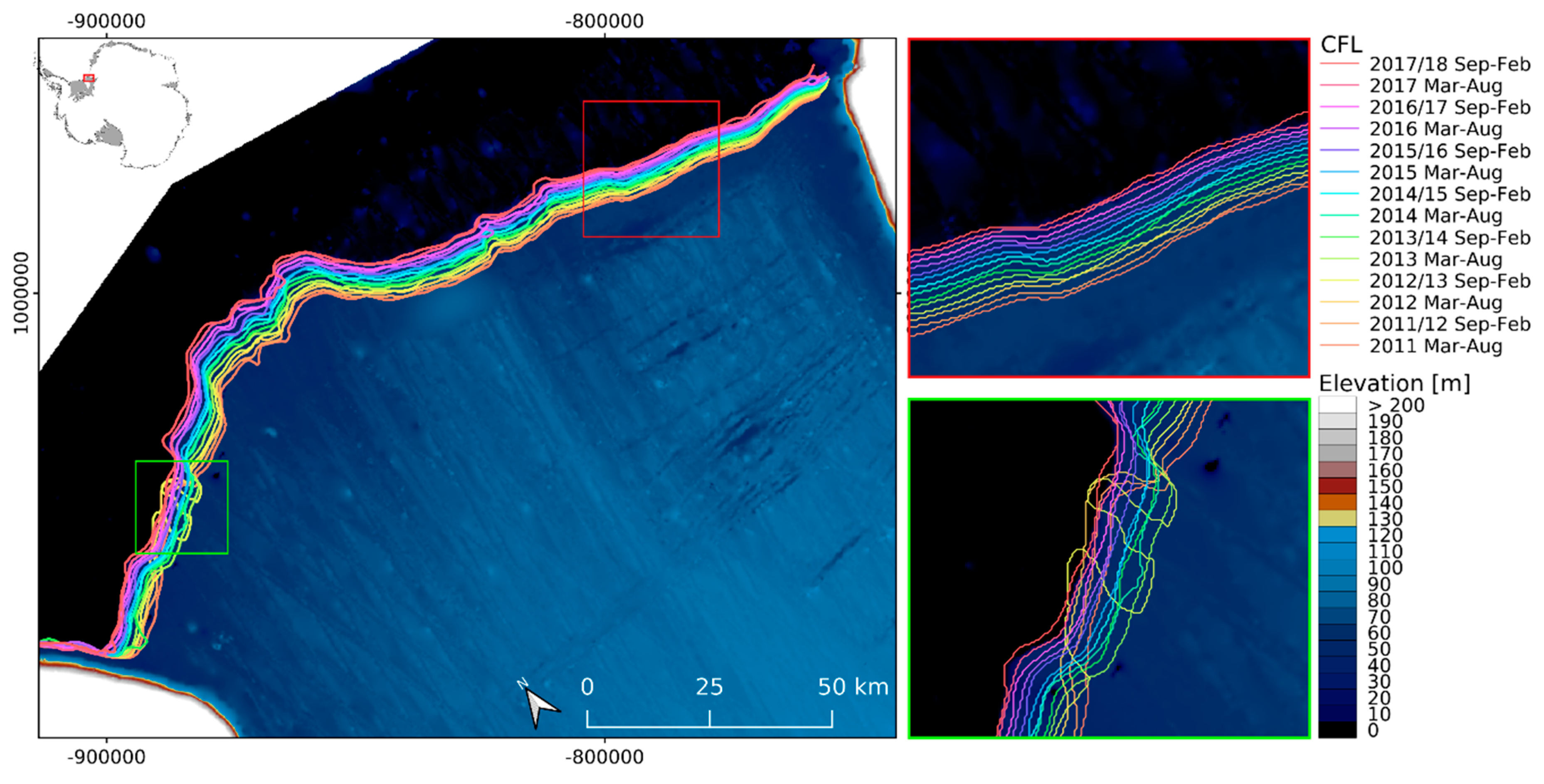
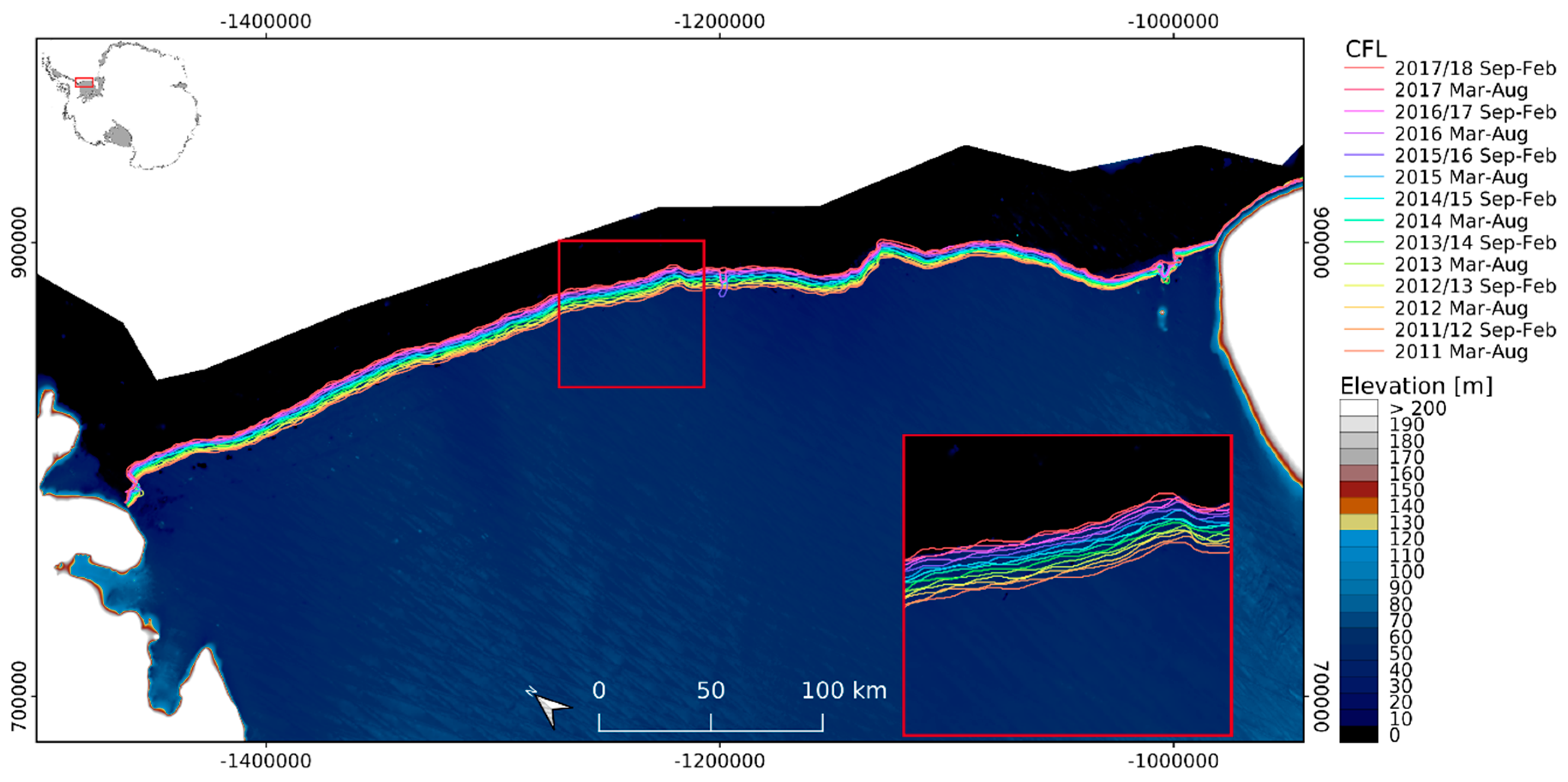
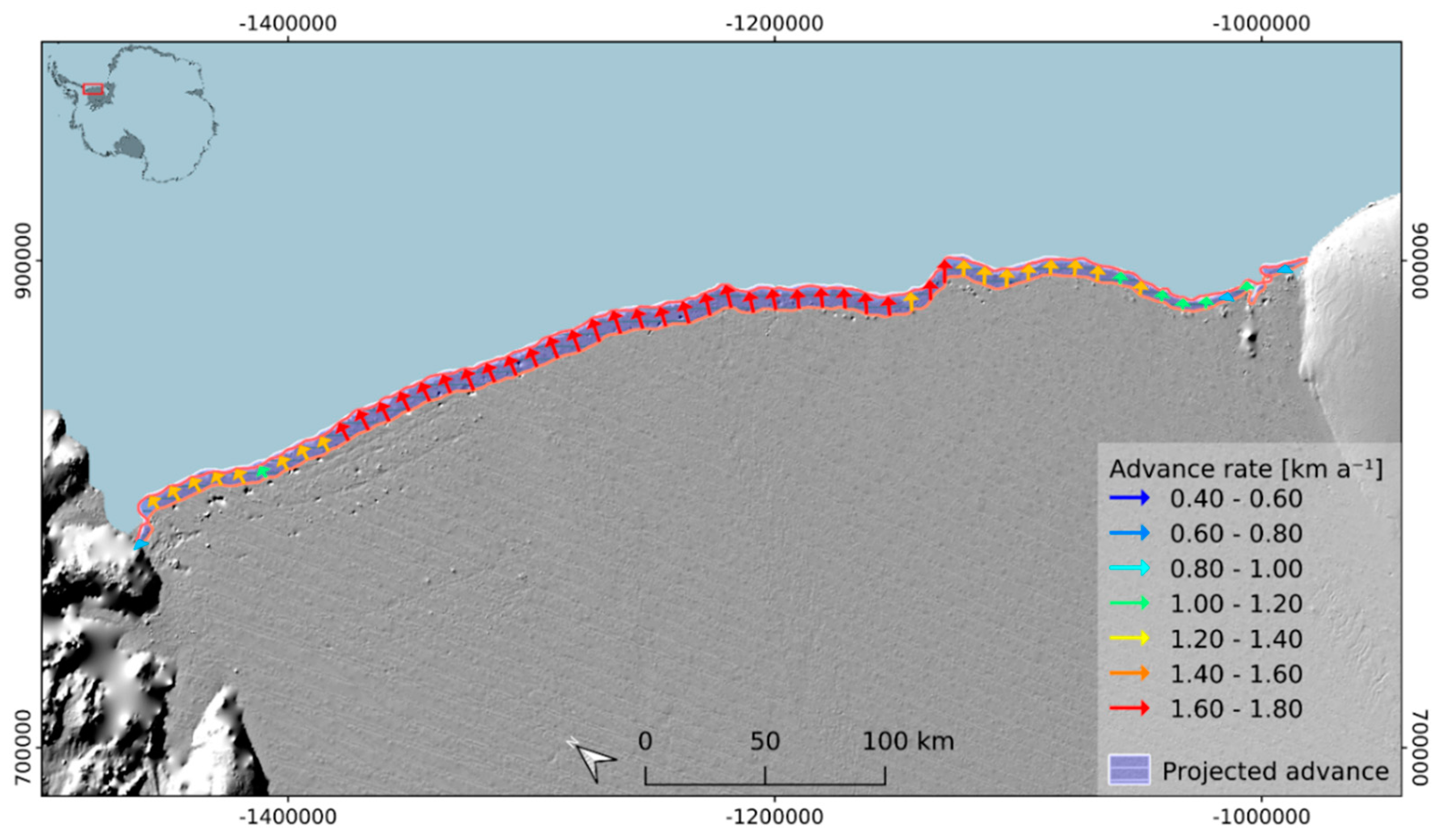
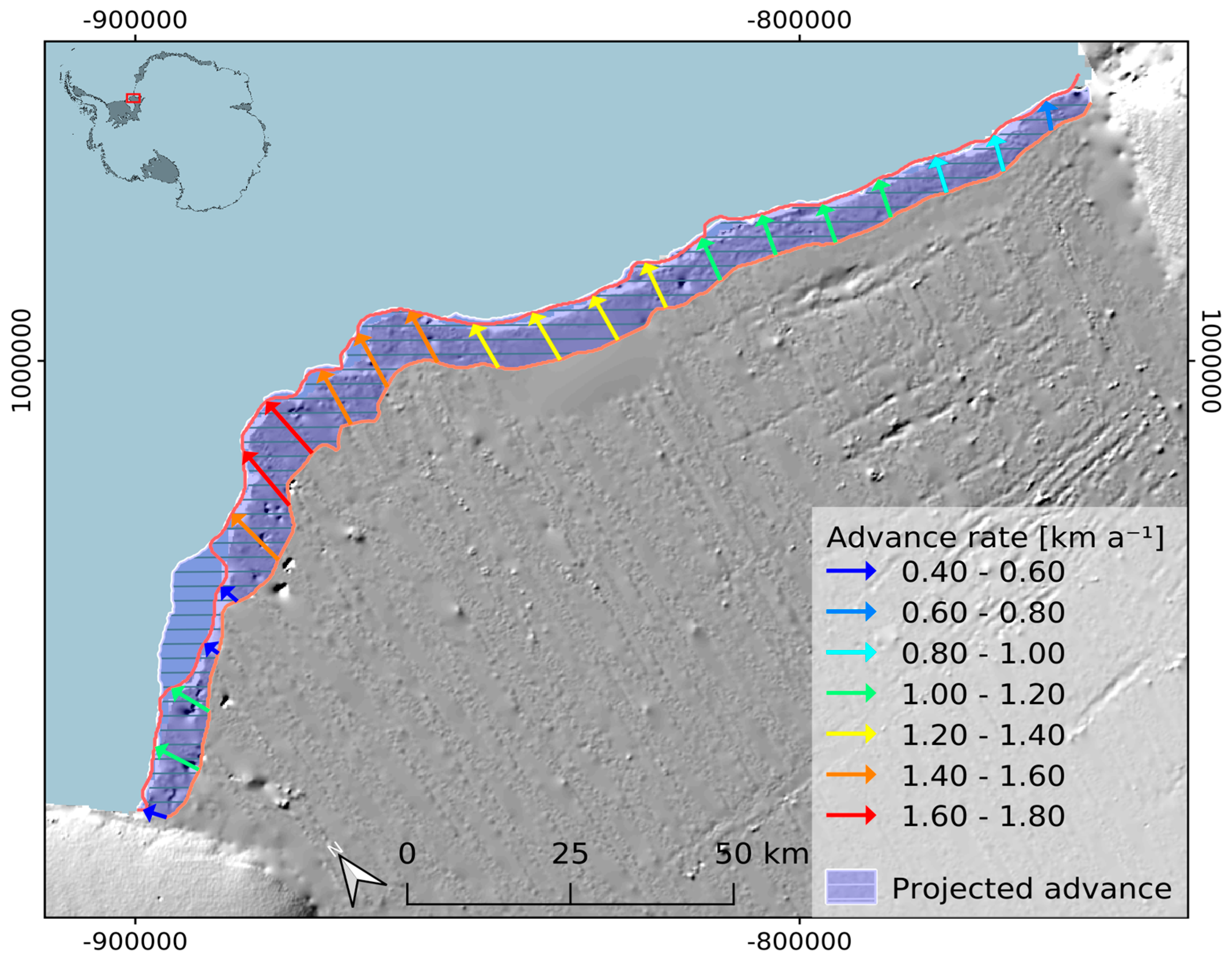
3.1. Calving Front Migration
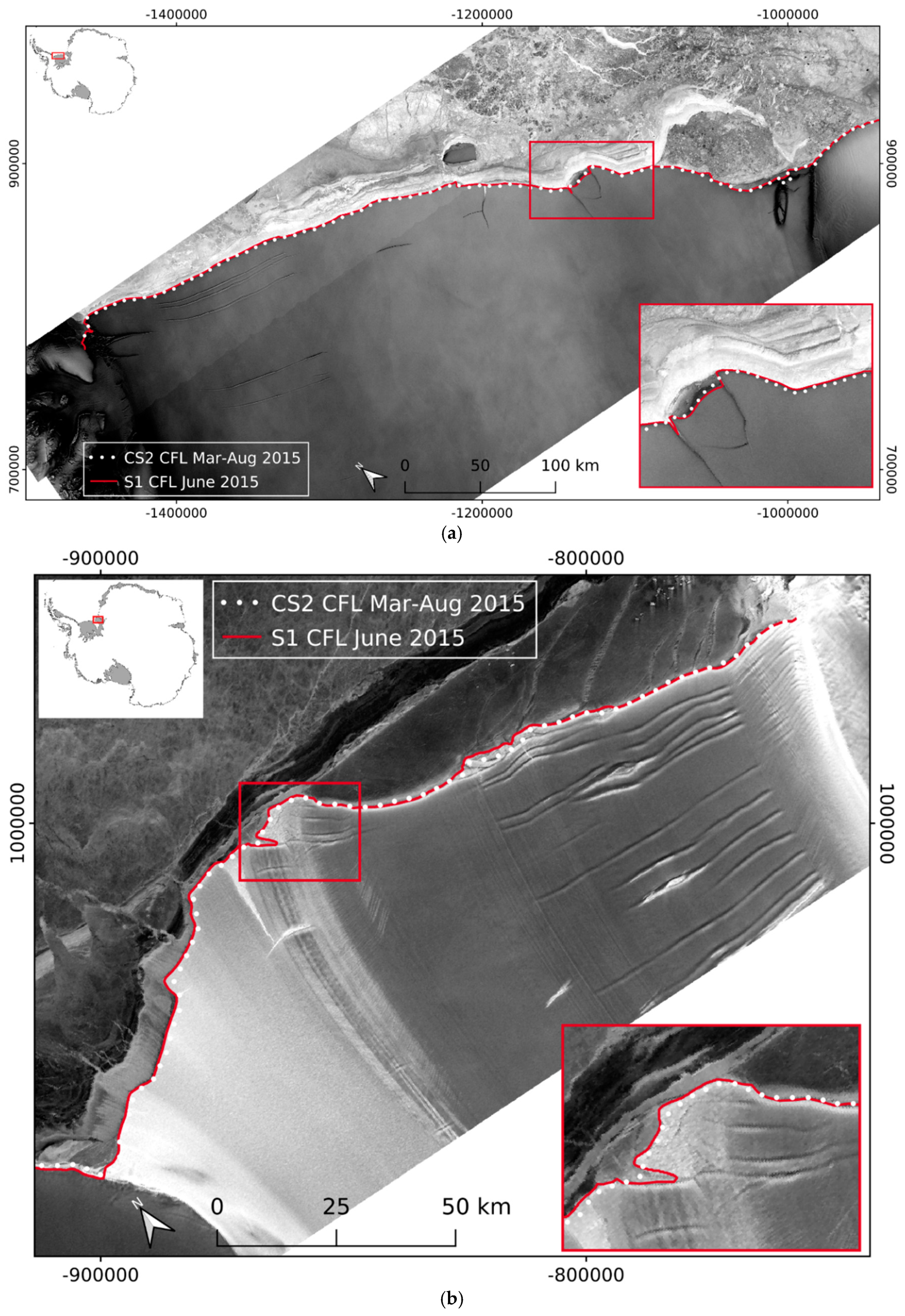
3.2. Intercomparison with Manually Derived CFLs from Sentinel-1
3.3. Area Change and Iceberg Calving Rate Results
4. Discussion
5. Conclusions
Author Contributions
Funding
Acknowledgments
Conflicts of Interest
Data Availability
References
- Depoorter, M.A.; Bamber, J.L.; Griggs, J.A.; Lenaerts, J.T.M.; Ligtenberg, S.R.M.; Van den Broeke, M.R.; Moholdt, G. Calving fluxes and basal melt rates of Antarctic ice shelves. Nature 2013, 502, 89–92. [Google Scholar] [CrossRef] [PubMed]
- Rignot, E.; Jacobs, S.S.; Mouginot, J.; Scheuchl, B. Ice-shelf melting around Antarctica. Science 2013, 341, 266–270. [Google Scholar] [CrossRef] [PubMed]
- Lazzara, M.A.; Jezek, K.C.; Scambos, T.A.; MacAyeal, D.R.; Van der Veen, C.J. On the recent calving of icebergs from the Ross Ice Shelf. Polar Geogr. 1999, 23, 201–212. [Google Scholar] [CrossRef]
- Hogg, A.E.; Gudmundsson, G.H. Impacts of the Larsen-C Ice Shelf calving event. Nat. Clim. Chang. 2017, 7, 540. [Google Scholar] [CrossRef]
- Rott, H.; Skvarca, P.; Nagler, T. Rapid collapse of Northern Larsen Ice Shelf, Antarctica. Science 1996, 271, 788–792. [Google Scholar] [CrossRef]
- Rack, W.; Rott, H. Pattern of retreat and disintegration of Larsen B Ice Shelf, Antarctic Peninsula. Ann. Glaciol. 2004, 39, 505–510. [Google Scholar] [CrossRef]
- Glasser, N.F.; Scambos, T.A. A structural glaciological analysis of the 2002 Larsen B ice-shelf collapse. J. Glaciol. 2008, 54, 3–16. [Google Scholar] [CrossRef]
- Rott, H.; Rack, W.; Skvarca, P.; De Angelis, H. Northern Larsen Ice Shelf, Antarctica: Further retreat after collapse. Ann. Glaciol. 2002, 34, 277–282. [Google Scholar] [CrossRef]
- De Angelis, H.; Skvarca, P. Glacier surge after ice shelf collapse. Science 2003, 299, 1560–1562. [Google Scholar] [CrossRef]
- Scambos, T.A.; Bohlander, J.A.; Shuman, C.A.; Skvarca, P. Glacier acceleration and thinning after ice shelf collapse in the Larsen B embayment, Antarctica. Geophys. Res. Lett. 2004, 31, L18402. [Google Scholar] [CrossRef]
- Scambos, T.A.; Berthier, E.; Shuman, C.A. The triggering of subglacial lake drainage during rapid glacier drawdown: Crane Glacier, Antarctic Peninsula. Ann. Glaciol. 2011, 52, 74–82. [Google Scholar] [CrossRef]
- Favier, L.; Pattyn, F.; Berger, S.; Drews, R. Dynamic influence of pinning points on marine ice-sheet stability: A numerical study in Dronning Maud Land, East Antarctica. Cryosphere 2016, 10, 2623–2635. [Google Scholar] [CrossRef]
- Fürst, J.J.; Durand, G.; Gillet-Chaulet, F.; Tavard, L.; Rankl, M.; Braun, M.; Gagliardini, O. The safety band of Antarctic ice shelves. Nat. Clim. Chang. 2016, 6, 479–482. [Google Scholar] [CrossRef]
- Baumhoer, C.A.; Dietz, A.J.; Dech, S.; Kuenzer, C. Remote Sensing of Antarctic Glacier and Ice-Shelf Front Dynamics—A Review. Remote Sens. 2018, 10, 1445. [Google Scholar] [CrossRef]
- Mottram, R.; Simonsen, S.B.; Svendsen, S.H.; Barletta, V.R.; Sandberg Sørensen, L.; Nagler, T.; Wuite, J.; Groh, A.; Horwath, M.; Rosier, J.; et al. An integrated view of Greenland Ice Sheet mass changes based on models and satellite observations. Remote Sens. 2019, 11, 1407. [Google Scholar] [CrossRef]
- Krieger, L.; Floricioiu, D. Automatic glacier calving front delineation on TerraSAR-X and Sentinel-1 SAR imagery. In Proceedings of the 2017 IEEE International Geoscience and Remote Sensing Symposium (IGARSS), Fort Worth, TX, USA, 23–28 July 2017; pp. 2817–2820. [Google Scholar] [CrossRef]
- Mohajerani, Y.; Wood, M.; Velicogna, I.; Rignot, E. Detection of Glacier Calving Margins with Convolutional Neural Networks: A Case Study. Remote Sens. 2019, 11, 74. [Google Scholar] [CrossRef]
- Liu, H.; Jezek, K.C. A Complete High-Resolution Coastline of Antarctica Extracted from Orthorectified Radarsat Sar Imagery. Photogramm. Eng. Remote Sens. 2004, 70, 605–616. [Google Scholar] [CrossRef]
- Liu, H.; Jezek, K.C. Automated extraction of coastline from satellite imagery by integrating Canny edge detection and locally adaptive thresholding methods. Int. J. Remote Sens. 2004, 25, 937–958. [Google Scholar] [CrossRef]
- Jezek, K.C. RADARSAT-1 Antarctic Mapping Project: Change-detection and surface velocity campaign. Ann. Glaciol. 2002, 34, 263–268. [Google Scholar] [CrossRef]
- Scambos, T.A.; Haran, T.M.; Fahnestock, M.A.; Painter, T.H.; Bohlander, J. MODIS-based Mosaic of Antarctica (MOA) data sets: Continent-wide surface morphology and snow grain size. Remote Sens. Environ. 2007, 111, 242–257. [Google Scholar] [CrossRef]
- Fricker, H.A.; Young, N.W.; Allison, I.; Coleman, R. Iceberg calving from the Amery Ice Shelf, East Antarctica. Ann. Glaciol. 2002, 34, 241–246. [Google Scholar] [CrossRef]
- Rignot, E. Ice-shelf changes in Pine Island Bay, Antarctica, 1947–2000. J. Glaciol. 2002, 48, 247–256. [Google Scholar] [CrossRef]
- Miles, B.W.J.; Stokes, C.R.; Jamieson, S.S.R. Simultaneous disintegration of outlet glaciers in Porpoise Bay (Wilkes Land), East Antarctica, driven by sea ice break-up. Cryosphere 2017, 11, 427–442. [Google Scholar] [CrossRef]
- Rott, H.; Abdel Jaber, W.; Wuite, J.; Scheiblauer, S.; Floricioiu, D.; Van Wessem, J.M.; Nagler, T.; Miranda, N.; Van den Broeke, M.R. Changing pattern of ice flow and mass balance for glaciers discharging into the Larsen A and B embayments, Antarctic Peninsula, 2011 to 2016. Cryosphere 2018, 12, 1273–1291. [Google Scholar] [CrossRef]
- Gourmelen, N.; Escorihuela, M.J.; Shepherd, A.; Foresta, L.; Muir, A.; Garcia-Mondéjar, A.; Drinkwater, M.R. CryoSat-2 swath interferometric altimetry for mapping ice elevation and elevation change. Adv. Space Res. 2018, 62, 1226–1242. [Google Scholar] [CrossRef]
- Chuter, S.J.; Bamber, J.L. Antarctic ice shelf thickness fromCryoSat-2 radar altimetry. Geophys. Res. Lett. 2015, 42, 10721–10729. [Google Scholar] [CrossRef]
- Rosier, S.H.R.; Hofstede, C.; Brisbourne, A.M.; Hattermann, T.; Nicholls, K.W.; Davis, P.E.D.; Anker, P.G.D.; Hillenbrand, C.-D.; Smith, A.M.; Corr, H.F.J. A new bathymetry for the southeastern Filchner-Ronne Ice Shelf: Implications for modern oceanographic processes and glacial history. J. Geoph. Res. Oceans 2018, 123, 4610–4623. [Google Scholar] [CrossRef]
- Hogg, A.E.; Shepherd, A.; Gilbert, L.; Muir, A.; Drinkwater, M.R. Mapping ice sheet grounding lines with CryoSat-2. Adv. Space Res. 2018, 62, 1191–1202. [Google Scholar] [CrossRef]
- Ferrigno, J.G.; Gould, W.G. Substantial changes in the coastline of Antarctica revealed by satellite imagery. Polar Rec. 1987, 23, 577. [Google Scholar] [CrossRef]
- MacAyeal, D.R.; Padman, L.; Drinkwater, M.R.; Fahnestock, M.; Gotis, T.T.; Gray, A.L.; Kerman, B.; Lazzara, M.; Rignot, E.; Scambos, T.; et al. Effects of Rigid Body Collisions and Tide-forced Drift on Large Tabular Icebergs of the Antarctic. 2002. Available online: http://geosci.uchicago.edu/~drm7/research/Icebergs_of_Y2k.pdf (accessed on 23 July 2019).
- Larour, E.; Rignot, E.; Aubry, D. Modelling of rift propagation on Ronne Ice Shelf, Antarctica, and sensitivity to climate change. Geophys. Res. Lett. 2004, 31, L16404. [Google Scholar] [CrossRef]
- Wingham, D.J.; Francis, C.R.; Baker, S.; Bouzinac, C.; Brockley, D.; Cullen, R.; De Chateau-Thierry, P.; Laxona, S.W.; Mallow, U.; Mavrocordatos, C.; et al. CryoSat: A mission to determine the fluctuations in Earth’s land and marine ice fields. Adv. Space Res. 2006, 37, 841–871. [Google Scholar] [CrossRef]
- Howat, I.M.; Porter, C.; Smith, B.E.; Noh, M.-J.; Morin, P. The Reference Elevation Model of Antarctica. Cryosphere 2019, 13, 665–674. [Google Scholar] [CrossRef]
- Gourmelen, N.; Goldberg, D.; Snow, K.; Henley, S.; Bingham, R.G.; Kimura, S.; Hogg, A.; Shepherd, A.; Mouginot, J.; Lenaerts, J.T.M.; et al. Channelized melting drives thinning under a rapidly melting Antarctic ice shelf. Geophys. Res. Lett. 2017, 44, 9796–9804. [Google Scholar] [CrossRef]
- Goldberg, D.; Gourmelen, N.; Kimura, S.; Millan, R.; Snow, K. How accurately should we model ice shelf melt rates? Geophys. Res. Lett. 2019, 46, 189–199. [Google Scholar] [CrossRef]
- Smith, W.H.F.; Wessel, P. Gridding with continuous curvature splines in tension. Geophysics 1990, 55, 293–305. [Google Scholar] [CrossRef]
- Mayer-Gürr, T.; Pail, R.; Gruber, T.; Fecher, T.; Rexer, M.; Schuh, W.-D.; Kusche, J.; Brockmann, J.-M.; Rieser, D.; Zehentner, N.; et al. The combined satellite gravity field model GOCO05s. Geophys. Res. Abstr. 2015, 17, 12364. [Google Scholar]
- Canny, J. A computational approach to edge detection. IEEE Trans. Pattern Anal. Mach. Intell. 1986, 8, 679–698. [Google Scholar] [CrossRef]
- Paterson, W.S.B. The Physics of Glaciers, 3rd ed.; Elsevier: Oxford, UK, 1994. [Google Scholar]
- Vieli, A.; Funk, M.; Blatter, H. Flow dynamics of tidewater glaciers: A numerical modelling approach. J. Glaciol. 2001, 47, 595–606. [Google Scholar] [CrossRef]
- Liu, Y.; Moore, J.C.; Cheng, X.; Gladstone, R.M.; Bassis, J.N.; Liu, H.; Wen, J.; Hui, F. Ocean-driven thinning enhances iceberg calving and retreat of Antarctic ice shelves. Proc. Natl. Acad. Sci. USA 2015, 112, 3263–3268. [Google Scholar] [CrossRef]
- Nagler, T.; Rott, H.; Hetzenecker, M.; Wuite, J.; Potin, P. The Sentinel-1 Mission: New Opportunities for Ice Sheet Observations. Remote Sens. 2015, 7, 9371–9389. [Google Scholar] [CrossRef]
- Ligtenberg, S.R.M.; Kuipers-Munneke, P.; Van den Broeke, M.R. Present and future variations in Antarctic firn air content. Cryosphere 2014, 8, 1711–1723. [Google Scholar] [CrossRef]
- Van den Broeke, M.; Van de Berg, W.; Van Meijgaard, E. Firn depth correction along the Antarctic grounding line. Antarct. Sci. 2008, 20, 513–517. [Google Scholar] [CrossRef]
- The IMBIE Team. Mass balance of the Antarctic Ice Sheet from 1992 to 2017. Nature 2018, 558, 219–222. [Google Scholar] [CrossRef] [PubMed]
- IPCC. Summary for Policymakers. IPCC Special Report on the Ocean and Cryosphere in A Changing Climate, Pörtner, H.-O., Roberts, D.C., Masson-Delmotte, V., Zhai, P., Tignor, M., Poloczanska, E., Mintenbeck, K., Nicolai, M., Okem, A., Petzold, J., et al., Eds.; 2019; In press. [Google Scholar]
- Dehecq, A.; Gourmelen, N.; Shepherd, A.; Cullen, R.; Trouvé, E. Evaluation of CryoSat-2 for height retrieval over the Himalayan range. In Proceedings of the CryoSat-2 Third User Workshop, Dresden, Germany, 12–14 March 2013. [Google Scholar]


© 2019 by the authors. Licensee MDPI, Basel, Switzerland. This article is an open access article distributed under the terms and conditions of the Creative Commons Attribution (CC BY) license (http://creativecommons.org/licenses/by/4.0/).
Share and Cite
Wuite, J.; Nagler, T.; Gourmelen, N.; Escorihuela, M.J.; Hogg, A.E.; Drinkwater, M.R. Sub-Annual Calving Front Migration, Area Change and Calving Rates from Swath Mode CryoSat-2 Altimetry, on Filchner-Ronne Ice Shelf, Antarctica. Remote Sens. 2019, 11, 2761. https://doi.org/10.3390/rs11232761
Wuite J, Nagler T, Gourmelen N, Escorihuela MJ, Hogg AE, Drinkwater MR. Sub-Annual Calving Front Migration, Area Change and Calving Rates from Swath Mode CryoSat-2 Altimetry, on Filchner-Ronne Ice Shelf, Antarctica. Remote Sensing. 2019; 11(23):2761. https://doi.org/10.3390/rs11232761
Chicago/Turabian StyleWuite, Jan, Thomas Nagler, Noel Gourmelen, Maria Jose Escorihuela, Anna E. Hogg, and Mark R. Drinkwater. 2019. "Sub-Annual Calving Front Migration, Area Change and Calving Rates from Swath Mode CryoSat-2 Altimetry, on Filchner-Ronne Ice Shelf, Antarctica" Remote Sensing 11, no. 23: 2761. https://doi.org/10.3390/rs11232761
APA StyleWuite, J., Nagler, T., Gourmelen, N., Escorihuela, M. J., Hogg, A. E., & Drinkwater, M. R. (2019). Sub-Annual Calving Front Migration, Area Change and Calving Rates from Swath Mode CryoSat-2 Altimetry, on Filchner-Ronne Ice Shelf, Antarctica. Remote Sensing, 11(23), 2761. https://doi.org/10.3390/rs11232761