Abstract
The Greenland ice sheet is a major contributor to sea level rise, adding on average 0.47 ± 0.23 mm year to global mean sea level between 1991 and 2015. The cryosphere as a whole has contributed around 45% of observed global sea level rise since 1993. Understanding the present-day state of the Greenland ice sheet is therefore vital for understanding the processes controlling the modern-day rates of sea level change and for making projections of sea level rise into the future. Here, we provide an overview of the current state of the mass budget of Greenland based on a diverse range of remote sensing observations to produce the essential climate variables (ECVs) of ice velocity, surface elevation change, grounding line location, calving front location, and gravimetric mass balance as well as numerical modelling that together build a consistent picture of a shrinking ice sheet. We also combine these observations with output from a regional climate model and from an ice sheet model to gain insight into existing biases in ice sheet dynamics and surface mass balance processes. Observations show surface lowering across virtually all regions of the ice sheet and at some locations up to −2.65 m year between 1995 and 2017 based on radar altimetry analysis. In addition, calving fronts at 28 study sites, representing a sample of typical glaciers, have retreated all around Greenland since the 1990s and in only two out of 28 study locations have they remained stable. During the same period, two of five floating ice shelves have collapsed while the locations of grounding lines at the remaining three floating ice shelves have remained stable over the observation period. In a detailed case study with a fracture model at Petermann glacier, we demonstrate the potential sensitivity of these floating ice shelves to future warming. GRACE gravimetrically-derived mass balance (GMB) data shows that overall Greenland has lost 255 ± 15 Gt year of ice over the period 2003 to 2016, consistent with that shown by IMBIE and a marked increase compared to a rate of loss of 83 ± 63 Gt year in the 1993–2003 period. Regional climate model and ice sheet model simulations show that surface mass processes dominate the Greenland ice sheet mass budget over most of the interior. However, in areas of high ice velocity there is a significant contribution to mass loss by ice dynamical processes. Marked differences between models and observations indicate that not all processes are captured accurately within models, indicating areas for future research.
1. Introduction
The Greenland ice sheet is a major contributor to present day observed sea level rise [1,2] and a changing Arctic climate will likely continue to have a profound impact on the ice sheet mass budget in the future. Greenland has been experiencing some of the highest rates of climate change on the planet [3], with observed temperature increases of 2 K since records began in the 1870s [4]. The contribution to sea level rise from the Greenland ice sheet is determined by the total mass budget that results from two main processes: the melt and runoff of surface snow and ice and a dynamic component due to iceberg calving and ice-ocean interactions at ocean terminating glaciers.
The mass budget of the ice sheet as a whole is driven by precipitation at the surface of the ice sheet, which is balanced at the surface by ice melt and runoff. As meltwater and rainfall over the surface snow can refreeze in the snowpack [5] or be retained in liquid firn aquifers or englacially, liquid water (from melt or rainfall) does not automatically run off and this significantly complicates the calculation of the surface mass balance (SMB). The SMB is also sometimes referred to as climatic mass budget or surface mass balance. The dynamic component of the mass budget is a mass loss component resulting from iceberg calving and ocean driven melting that has been only relatively poorly observed in the field (for example., [6]). More minor contributions to the mass budget come from basal melting but this process is not considered in detail here.
The relative contribution to the total mass budget of the two main components of the budget is important as it determines both the regional sea level rise fingerprint and the rate at which the ice sheet can respond to further climate change. The ice sheet’s total mass change has been estimated using a range of different methods including radar and laser altimetry, synthetic aperture interferometry as part of the mass budget method and gravimetry. In the first Ice Sheet Mass Balance Inter-comparison Exercise (IMBIE, [2]), the average Greenland mass budget from four independent methods was −237 Gt year between 2000 and 2011, which is a contribution of 0.65 mm year to mean sea level rise; and −263 Gt year between 2005 and 2011, which is a contribution of 0.72 mm year to mean sea level rise. This accounts for a little less than a third of the average 3.1 mm year observed sea level rise between 1993 and 2017. As each measurement technique is sensitive to different processes and there is high inter-annual variability in precipitation, melt, calving fluxes and other processes, the total mass budget of the Greenland ice sheet is sensitive to the time period chosen and methods used including also assumptions about for example, glacio-isostatic adjustments, definition of basins, models used for data interpretation and many other processes as for example noted by Enderlin et al. [7]. In addition, measurement uncertainties as well as the reliance on numerical models of key processes such as SMB leads to significant uncertainty in estimates of total mass budget. Among other factors, SMB derived from regional climate models is reliant on model physics that determine how much precipitation falls and where [8]. Precipitation is also strongly influenced by model resolution [9]. Radiation schemes largely determine how much snow and ice melts and these are highly sensitive to cloud parameterisation choices [10,11] and albedo [5,12] as well as model resolution and choice of boundary forcing. Even simple choices such as of ice sheet masks and which topographic datasets are used have significant impact on estimates of SMB [13]. As SMB is used to force ice sheet models, the uncertainties can propagate into ice sheet models as for example shown by Adalgeirsdottir et al. [14]. The use of models is necessary to interpret remotely sensed data and in particular for partitioning mass change by different processes. Improving models is complicated by a lack of ground-based observation stations, especially over longer time scales. For this reason, the availability of remote sensing observations is vital to monitoring the present status of the ice sheet as well as for initialising and assimilating into models. There has however, been a significant increase in the amount of data available within the earth sciences including in and around the Greenland cryosphere in recent years as documented by for example the Promice (Programme for monitoring the Greenland ice sheet) automatic weather stations on the ice sheet as well as the NASA MEaSUREs data and IceBridge (e.g., [7,15]).
In this article we summarise the current state of Greenland ice sheet mass balance and evaluate the importance of different ice sheet processes, whether resulting from ice sheet dynamics, surface mass balance or submarine melt using both observations and numerical models. The European Space Agency’s climate change initiative (ESA CCI) for the Greenland ice sheet has made available extensive pre-processed remotely sensed datasets for scientific research. By consolidating, standardising and integrating satellite remote sensing data, high quality datasets are now accessible to scientists, policymakers and other stakeholders. This data has been used to identify significant trends and changes in ice dynamics in Greenland including identifying significant changes in ice velocity at large outlet glaciers [16], assessing the causes of surface elevation change across the ice sheet [17,18,19,20] as well as assessing the importance of different processes controlling seasonal velocity changes on the ice sheet [21]. The availability of this data is invaluable in communicating the effects of climate change on the cryosphere and the likely impacts on sea level rise and human societies. The essential climate variables (ECVs) specific to Greenland focus attention on the most significant processes that lead to changes in ice sheet properties and therefore sea level rise. They allow both detailed process studies and are a monitoring tool to determine the present day state of the Greenland ice sheet. They also indicate the likely direction of future evolution and sources of uncertainty, particularly when combined with regional climate and ice sheet model outputs. Surface elevation change (SEC) reflects changes in both mass input from snowfall and mass output from melt and runoff as well as the importance of dynamical changes leading to drawdown or thickening of ice related to changes in ice velocity (IV). Calving front location (CFL) and grounding line location (GLL) at floating glacier termini reflect glacier retreat rates that can be driven by both ocean processes and internal ice dynamics. Gravimetrically derived mass balance (GMB) data ties all of these processes together and can give an overall ice sheet and basin scale estimate of total mass change. All remote sensing data and model output is available for download (see Supplementary materials). Combining these datasets with numerical models is a powerful means of partitioning observed changes by different processes in order to both assess the baseline of ice sheet changing and the likely factors driving ice sheet mass loss. A number of scientific studies have already published important results for Greenland based partly or fully on the Greenland ice sheet CCI data [18,19,20,22], but combining the observations with numerical modelling reveals the power of the dataset to clarify important and outstanding issues in Greenland ice sheet science. Aside from simple model evaluation using satellite data, the use of numerical models in combination with satellite observations takes three forms in this study. Firstly, we use model outputs to estimate and correct the direct contribution of different physical processes to mass budget, for example by using solid and liquid precipitation, melt, sublimation, evaporation and temperature derived from a high resolution regional climate model, to correct surface elevation change data for firn compaction [23] and convert into altimetric mass balance [17]. Secondly, we use observational data in combination with models to infer the importance of second order processes, for example by comparing surface mass balance derived from RCMs with GMB data. This allows us to partition mass loss from the Greenland ice sheet on a basin scale and to assess where improvements in modelling processes important for ice sheet mass budget need to be made. Thirdly, we use observational data to drive model projections, for example with the use of ice velocity data to drive models of ice fracture and iceberg calving. These hybrid model-data products show great potential in improving estimates of sea level rise, both rate and magnitude, derived from ice sheet models and RCMs.
2. Methods and Datasets
In this paper we briefly review the five main data products developed in the CCI project and describe the techniques used to derive them. We also give a brief introduction to the RCM HIRHAM5 and the ice sheet model PISM used in the analysis and application of the data. In combination with ice dynamics modelling and regional climate modelling, the observations allow us to assess the present state of the Greenland ice sheet and partition the contribution of different processes, and regions of Greenland, to sea level rise as well as indicating uncertainties in model formulations and arising due to inadequate process understanding.
2.1. Ice Velocity
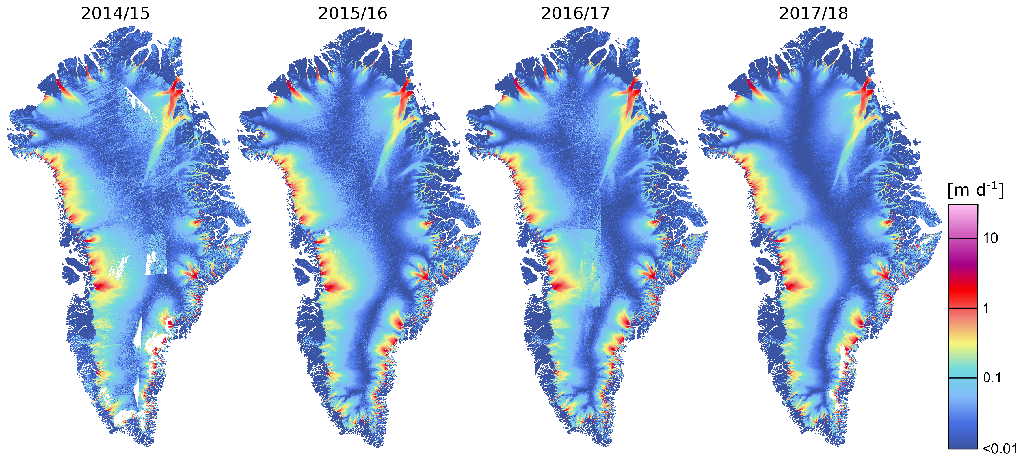
The annual velocity maps and ice velocity time series of outlet glaciers provide essential information for studying temporal fluctuations and long-term trends. They also provide key input for ice dynamic and climate modelling. The data set produced by the CCI has a high temporal resolution with multiple repeats giving high quality data over the ice sheet and outlet glaciers. Within the framework of the ESA CCI programme, a system for automatic generation of ice velocity maps from repeat pass Copernicus Sentinel-1 SAR data was developed [22]. The systematic acquisition planning of Sentinel-1 in Greenland is designed to cover the entire ice sheet margin at repeat intervals of 6 to 12 days augmented by annual ice sheet-wide winter campaigns. Taking advantage of this, annual ice velocity maps of the Greenland ice sheet as well as continuous time series of major outlet glaciers have been produced covering the entire Sentinel-1 period (2014–present). Ice motion is derived from Sentinel-1 Single Look Complex (SLC) image pairs acquired in Interferometric Wide (IW) swath mode applying both coherent and incoherent iterative offset tracking. The IW mode is the standard operation mode over land surfaces including inland ice. Applying Terrain Observation by Progressive Scans (TOPS) acquisition technology, it provides a spatial resolution of about 3 m × 22 m in slant range and azimuth, respectively, with a swath width of 250 km. Ice velocity maps with 250 m grid spacing are produced at 6- to 12-day intervals and are annually combined and averaged to compile a virtually gapless mosaic of ice sheet-wide mean velocity. Annual maps run from October to October and are thus equivalent to a glaciological SMB year. To date three consecutive annual Sentinel-1 IV maps have been produced as part of Grennland ice sheet CCI. Production of the 2017/18 map is pending but the 2017/18 winter campaign map is finished (Figure 1). The maps provide detailed snapshots of contemporary ice flow in Greenland.
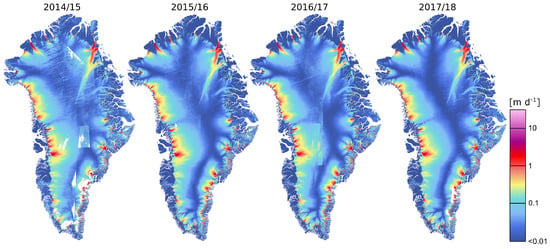
Figure 1.
Greenland ice sheet climate change initiative (CCI) annual ice velocity maps derived from Sentinel-1 SAR data 2014–2017 and winter campaign map 2017/18.
Quality assessment of the IV retrieval algorithm was performed through internal consistency checks (for example, checking how the algorithm performs on bedrock outcrops that are assumed stationary), and intercomparisons with other algorithms through a dedicated round-robin [24]. The velocity data is validated against independent datasets from ground-based in-situ GPS, higher resolution sensors (TerraSAR-X and COSMO-SkyMed) and available published datasets (MEaSUREs, e.g., [3,25]. A pixel-by-pixel intercomparison with the latest available winter campaign map 2017/18 shows a mean bias of 0.001 m/d and an RMSE of 0.04 m/d for both easting and northing components based on more than 33 million pixels [26].
2.2. Calving Fronts
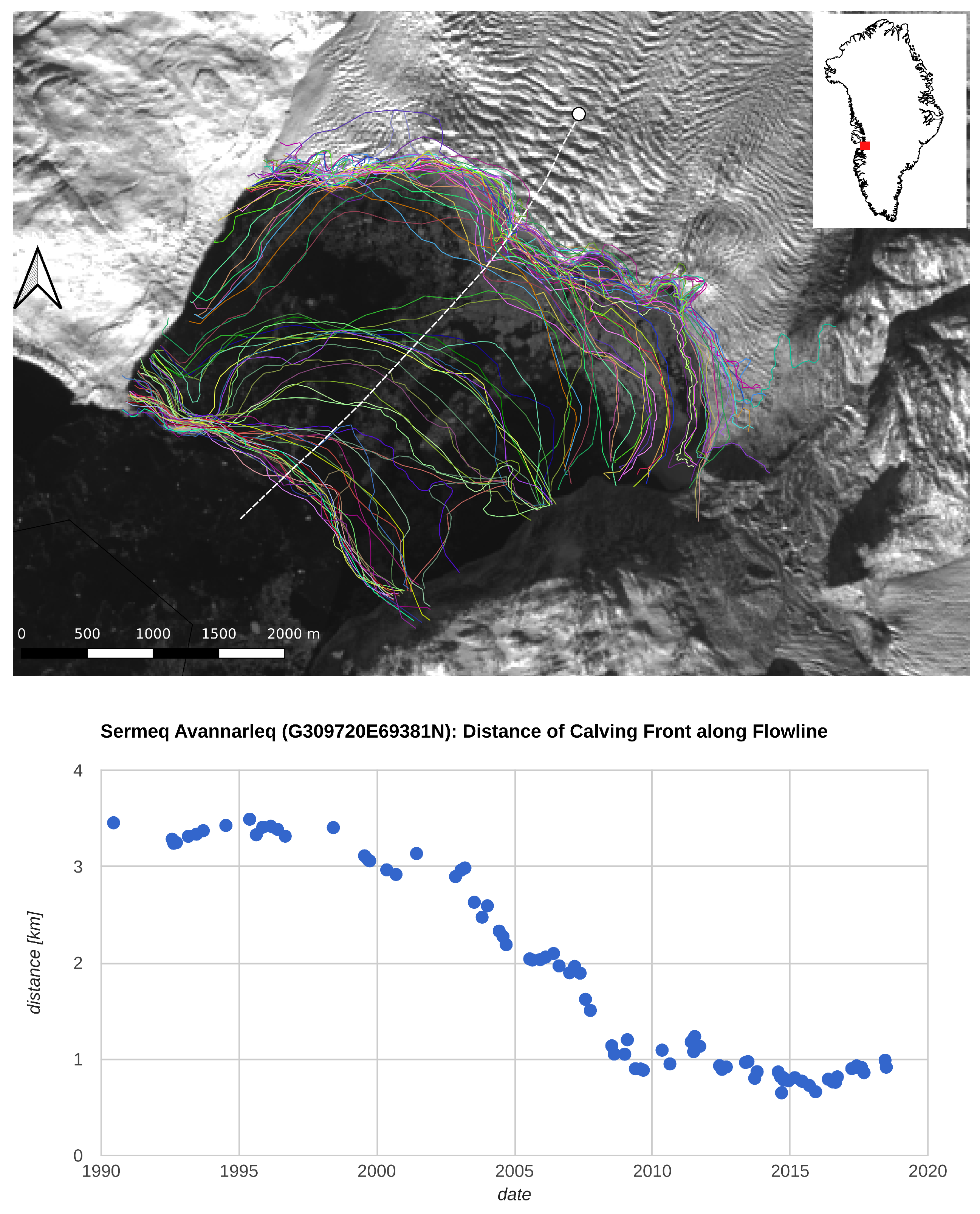
The calving front location (CFL) marks the ever-changing terminus position of a tidewater glacier subject to ice advance and iceberg calving [27]. The CFL is a basic glacier parameter, required for purposes such as mapping glacier extent, calculating areal change or calving rates and as model domain boundary. Monitoring CFL temporal evolution is important as prolonged retreat of the calving front is a sign of changing boundary conditions and/or dynamic instability. The CFL product covers 28 key outlet glaciers around the Greenland perimeter and nearly three decades in time (1990–present). Calving fronts are extracted, at annual to seasonal intervals, through manual delineation of the ice-ocean boundary using geocoded satellite images in a GIS environment. Source data include primarily SAR imagery (ERS-1/2, Envisat, ALOS PALSAR, Sentinel-1), with temporal gaps filled using optical data (Landsat-5/7/8, Sentinel-2). The nominal ground resolution of the images varies between 10–30 m. To assure accurate geocoding and avoid systematic shifts in CFL of glaciers subject to strong elevation changes, the CFL is in reference to a stationary geoid (EGM96) rather than topographic height from a DEM. CFLs are available as a collection of annotated shapefiles, with detailed metadata on, amongst others, sensor and ice conditions, in the Greenland ice sheet CCI database (see link at the end of the paper). Figure 2 shows an example of the CFL product for Sermeq Avannarleq glacier in West Greenland, depicted on a Landsat-8 image as well as time sequence of the ice front along a flowline. Prolonged retreat of the glacier terminus started in the late 1990s and it stabilized in 2010 at a new location approximately 2.5 km upstream. Errors in extracted ice fronts are generally within a few pixels and depend on factors such as sensor resolution and geocoding but also the seasonal presence of ice mélange in front of the glacier, which can hamper the detection of the ice front. Seasonal signals of retreat and readvance are also seen at many of these glacier fronts, making the long time series invaluable in assessing the state of the glacier dynamics.
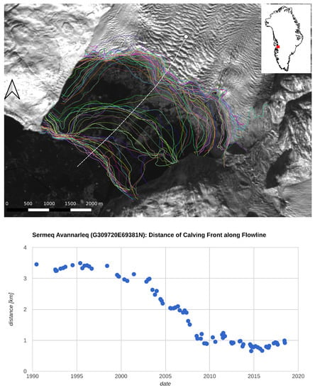
Figure 2.
(Top) CFLs of Sermeq Avannarleq Glacier in West Greenland from 1990 to 2018 shown as coloured lines (background: Landsat-8 image acquired at 7 October 2014, USGS). (Bottom) temporal evolution of CFL plotted as distance along the central flowline (dashed white line in left figure).
2.3. Grounding Lines
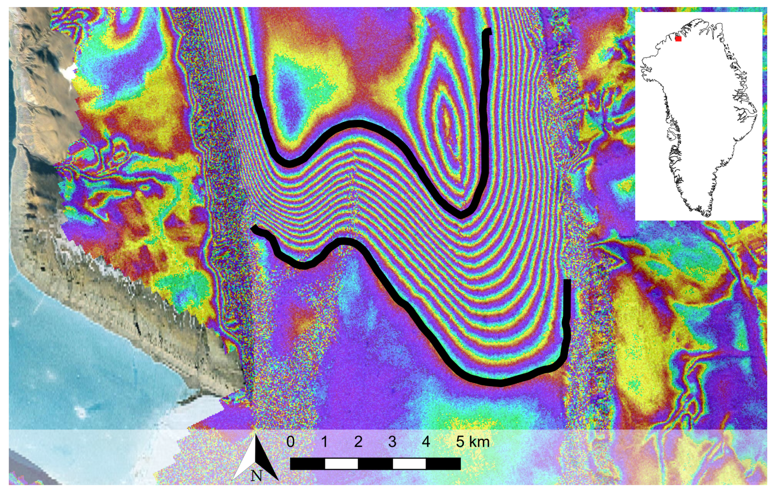
The Greenland ice sheet CCI project provides grounding line locations (GLL) for five key glaciers with floating termini in north Greenland: 79 glacier (also known as Nioghalvfjerds glacier), Hagen, Petermann, Ryder and Zachariæ Isstrøm. The grounding line marks the transition from grounded to floating ice and, particularly in basins with large overdeepenings, is a sensitive indicator of the stability of outlet glaciers [28]. The collapse of large floating ice shelves can lead to substantial acceleration and rapid retreat of outlet glaciers with a coincident increase in ice sheet mass loss [29]. Locating the grounding line is therefore critical for determining the mass flux of a marine based outlet glacier or ice sheet and monitoring changes in grounding line positions allows us to identify unstable regions. The GLL product is derived from InSAR data by mapping the lower and upper boundaries of the tidal flexure zone visible in double difference interferograms. These boundaries mark the seaward and landward limit of the tidal flexure zone respectively and serve as a proxy for the grounding zone [30,31]. Repeat pass data of ERS-1/2 acquired in 1995–1996 and Sentinel-1A (2015–2018) were used to map the grounding zone of the glaciers at two distinct epochs. The accuracy depends primarily on grounding zone geometry (slope), tidal amplitude, ice flow velocity and the quality of the interferogram (SNR, coherence, feature clarity) and uncertainties vary from 200 m to locally more than 1.5 km [32]. Improved precision can be achieved if multiple interferograms are available; however, it is difficult to separate between horizontal displacement due to ice flow and vertical displacement due to the tidal signal, especially on fast moving outlets. The launch of Sentinel-1B, in April 2016, has reduced the repeat pass period of the Sentinel-1 mission from 12 to 6 days reducing temporal decorrelation and providing significant improvements. We apply advanced interferometric processing, using pre-determined IV to aid the co-registration, in the formation of interferograms from Sentinel-1 TOPS mode data to account for the 6- to 12-day image acquisition interval and high flow speed (up to 3 m). Figure 3 shows an interferogram of the grounding zone of Ryder Glacier in north Greenland derived from 6-day repeat pass SAR data of Sentinel-1A and 1B acquired at 6, 12 and 18 January 2017. The grounding zone can be recognized as a distinct band of fringes in the interferogram caused by tidal deformation around a hinge as also shown by Hogg et al. [16].

Figure 3.
Geocoded double difference interferogram of the grounding zone of Ryder Glacier derived from repeat pass SAR data of Sentinel-1A and 1B acquired at 6, 12 and 18 January 2017 (background: Google Earth). Thick black lines indicate the lower and upper boundary of the tidal flexure zone. Inset shows location of Ryder Glacier in North Greenland.
2.4. Surface Elevation Change
The surface elevation change (SEC) dataset is based on satellite radar altimeter observations from satellites ERS-1, ERS-2, Envisat and Cryosat-2, covering the period of 1992–2017. The time series of observations is averaged as 5-year running mean estimates, to smooth interannual variability due to weather. The SEC estimation uses a mission specific combination of cross-over-, repeat-track- and least-squares-methods to estimate the temporal evolution of surface elevation at a common 5 km uniformed grid for the entire Greenland ice sheet. Full details in the mission specific set-up for deriving surface elevation change including errors are given in the the review of Sandberg Sørensen et al. [20]. If the reader is interested in more mission specific papers we refer to Sørensen et al. [18,19,33,34,35,36]. The observed SEC is compared with RCM and ISM results (see Section 3.1 and Section 3.3) to infer the importance of different processes.
2.5. Gravimetric Mass Balance from GRACE
The ESA Greenland Ice Sheet CCI provides estimates of ice mass balance derived from the joint NASA/DLR GRACE (Gravity Recovery & Climate Experiment) mission [37]. Operational between 2002 and 2017, the GRACE mission consisted of two identical spacecrafts flying about 220 km apart in a polar orbit originally at 480 km above the Earth, mapping the Earth’s gravity field each month. GRACE (and its successor GRACE-FO) is the only remote sensing sensor that directly measures total mass change, and thereby observes the total ice mass balance (or equivalent sea-level rise). The monthly solutions (level 2 products) are provided as spherical harmonic coefficients by different processing centres such as CSR (Center for Space Research at University of Texas, Austin, TX, USA), GFZ (GeoforschungsZentrum Potsdam, Germany), JPL (Jet Propulsion Laboratory, Pasadena, California, USA ) and more recently also by the Technical University of Graz (ITSG-Grace2016). The maximum spherical harmonic degree varies between the processing centres and releases (e.g., degree and order 60/96 for CSR RL06 or 60/90/120 for ITSG-Grace2016). As part of the ESA Greenland ice sheet CCI project, gravimetrically derived mass balance, also known as gravimetric mass balance (GMB), products are generated using both ITSG-Grace2016 [38] (2002–2017) and the new CSR RL06 solutions [39] (2003–2016). Moreover, independent GMB products are prepared by DTU Space (DTU) and TU Dresden (TUDR) using different approaches. The GMB products comprise mass change time series for eight drainage basins [40] and the entire Greenland ice sheet as well as gridded mass balance estimates over running 5-year periods.
DTU applies an inversion technique to derive monthly mass changes. Gravity observations at satellite altitude are used to solve for point masses on an icosahedron grid, where each point mass represents an area with a radius of ∼20 km. The ice mass changes over the whole Greenland ice sheet are derived including the peripheral glaciers, which cannot discriminate in the ∼300 km resolution of GRACE. A detailed description of the approach is given in Barletta et al. [41]. TUDR estimates monthly mass changes by applying a regional integration approach per grid cell of a km2 grid. For each grid cell a tailored sensitivity kernel was designed, which minimizes the sum of GRACE errors, derived from empirical error variance-covariance information, and signal leakage [42]. Mass change time series per drainage basin are derived by simply integrating the corresponding point masses or grid cells.
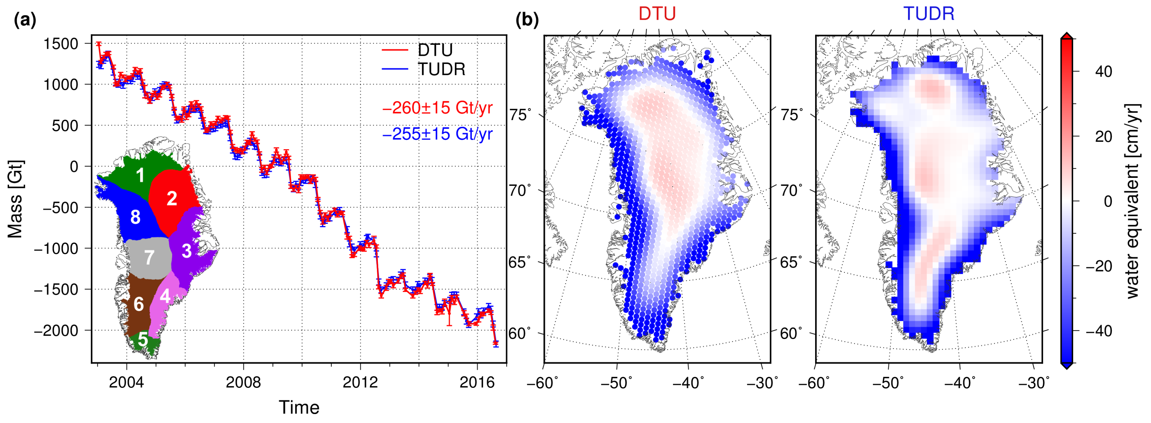
Figure 4 shows two types of GMB products derived by the different approaches and based on the CSR RL06 solution series (maximum degree and order 96). Differences in the spatial patterns of the 5-year trends originate from differing degrees of smoothing inherent to the applied methodologies. Nevertheless, the mass balance estimates, i.e., linear trends, for the entire Greenland ice sheet agree within their uncertainties. Trend differences are largely caused by differing GIA model corrections applied in both products. While DTU has applied the model by [43] based on the ICE-5G deglaciation history, TUDR has applied the ICE-6G(VM5a) [44] model prediction. Both model corrections differ by −6.3 Gt year for the entire Greenland ice sheet. Comparable products derived from the ITSG-Grace2016 solutions exhibit a high level of agreement compared to the CSR-based products, for example, the Greenland ice sheet mass balance estimates from both DTU products (based on CSR RL06 and ITSG-Grace2016) differ by only 3 Gt year.
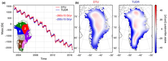
Figure 4.
GMB products provided by the ESA Greenland ice sheet CCI project. (a) Mass change time series for the entire Greenland ice sheet generated by DTU (red) and TUDR (blue). (b) Ice mass trends for 2007–2011 provided by DTU (left) and TUDR (right). All products are based on monthly solutions from the CSR RL06 series. Numbers indicate mass balance estimates and the corresponding uncertainties.
2.6. Regional Climate Model HIRHAM5
The Regional Climate Model HIRHAM5 as described in Langen et al. [5], Mottram et al. [45] is used in this study as climate forcing. Published studies (e.g., Enderlin et al. [46], Sasgen et al. [47], van den Broeke et al. [7]) use surface mass balance estimates derived from regional climate models such as RACMO, MAR and HIRHAM to assess the relative importance of surface and dynamic processes to ice sheet mass change by subtracting discharge of ice from modelled surface mass balance. The relatively high resolution and reasonable performance of such SMB models means that basin scale ice dynamics can in principle be resolved for the Greenland ice sheet by comparing GMB with SMB. In this study we compare the results from the HIRHAM5 RCM with published results from the RACMO2.3 RCM [1,47]. HIRHAM5 is run at 0.05 degrees (5.5 km) resolution on a rotated polar grid, and forced on the lateral boundaries with temperature, relative humidity, wind components and pressure at all 31 levels in the atmosphere every 6 hours from the ERA-Interim climate reanalysis dataset [48]. At the lower model boundary, sea surface temperatures and sea ice are applied daily and are also derived from ERA-Interim data. The climate model was developed at the Danish Meteorological Institute with physical schemes modified from ECHAM5 physics [49] to be suitable for application in polar regions [50,51]. The dynamical equations are derived from the HIRLAM7 numerical weather prediction model in both HIRHAM and RACMO [52] but they have different physics schemes [53]. The atmospheric radiative and turbulent fluxes drive a surface energy balance model to calculate melt rates. The SMB is calculated from the sum of the precipitation, sublimation and evaporation and runoff. The SMB model includes a multi-layer firn model that accounts for retention and refreezing of meltwater within the snowpack [5,51]. The effects of retention and refreezing are important to account for in calculating surface elevation change as well as having implications for total mass balance. As melt, that can be detected for example by passive microwave sensors [54], can refreeze or be retained within the snowpack and firn layers, the total melt generated does not necessarily lead to surface runoff or a mass loss from the system. Modelled SMB combined with GMB allows the partitioning of mass loss from Greenland into atmospherically driven melt and runoff and dynamically influenced calving and basal melt [2,47,55,56].
In this study we also use the SMB calculated in HIRHAM5, together with surface temperatures, to force the parallel ice sheet model (PISM). Ice sheet models are used to derive rates of dynamic mass change and are typically forced with a simplified surface forcing based on temperature and precipitation or, as in this study with a physically based SMB model using a surface energy budget method.
2.7. Ice Sheet Modelling with PISM
Given the vast amount of feedback mechanisms and interactions involving ice sheets in the climate system, ice sheet modelling and estimating future rates of ice loss is a major challenge [57,58]. Ice sheet dynamics have been identified as a major source of uncertainty in sea level rise projections by IPCC authors in the fifth assessment report [3]. Ice sheet models are available at a range of different degrees of complexity, including simpler shallow ice and shallow shelf models through higher order Blatter-Pattyn formulations to Full-Stokes ice sheet models [29,59]. Each model type has different limitations and strong points and is suitable for different types of simulations spanning a variety of temporal and spatial scales. Regardless of model complexity, proper boundary and initial conditions are necessary. These require high-quality observational data to be available. In addition, in order to validate the models and constrain model parameters, observational data sets are essential. Here, we use ice velocity and surface elevation data to evaluate simulations of the ice sheet with the Parallel Ice Sheet Model (PISM).
PISM is an open-source thermodynamically coupled, polythermal hybrid stress balance ice sheet model [60,61], which combines the Shallow Ice Approximation (SIA) [62] and the Shallow Shelf Approximation (SSA) [63,64]. We used an experimental set-up and values for the flow law determined by detailed experiments carried out by Aschwanden et al. [65]. The effective viscosity of glacier ice, , is given by
E is the flow enhancement factor, is the effective stress, A is the enthalpy-dependent rate factor and is a small constant regularizing the flow law at low effective stresses, thereby avoiding problems with infinite viscosity at zero deviatoric stress. For the simulations presented here, and for both the SIA and the SSA case (following the calibration by Aschwanden et al. [65]). In PISM, the flow velocity is given as a combination of the velocities according to the Shallow Ice Approximation (SIA), , and the Shallow Shelf Approximation (SSA), , [64];
where and
Calving is accounted for using a mask reflecting the initial ice geometry but with no further ice dynamical feedback implemented in the model. In order to examine the effects of sliding on the ice flow, different values for the yield stress of the basal till have been tested, from a value of Pa to Pa, the former being a very strong value, that ensures little or no sliding to amplify the flow [66]. All other model parameters related to sliding are kept constant.
The ice sheet model is run over Greenland at a uniform 2 km grid resolution, optimised for model performance within computational resource constraints. The effect of grid resolution on outlet velocities has been examined by Aschwanden et al. [65], who concluded that, in general, outlet velocity improves with smaller resolution and a minimum grid resolution of 2 km is needed in order to obtain correct orders of magnitude for the fast-flowing outlets. Initial bedrock and ice surface topography is from Bamber et al. [67] and the model is driven by monthly fields of surface mass balance and 2 m temperatures from the regional climate model HIRHAM5 (Section 2.6) for the period 1980–2017. Boundary conditions at the ice-ocean interface are constant in both space and time. Sub-shelf ice temperature is set to pressure-melting point and the sub-shelf melt rate is assumed to be proportional to a constant heat flux from the ocean into the ice. Prior to the 1980–2017 simulation, we made a spinup simulation consisting of a glacial cycle run following the SeaRISE experiments [68] at 10 km grid resolution followed by runs at progressively higher model resolution (10 km–5 km–2 km). Test runs with constant forcing changing only resolution of model (and forcing fields) and allowing bed topography to reflect the resolution change typically show a short transient with a quite steep decrease in ice mass when resolution changes, reflecting an increase in the number of resolved outlets. During spinup, the model is run until the ice mass is stable for each resolution. PISM is driven at the surface boundary by a constant annual cycle based on multi-year monthly means of the first 15 years of the HIRHAM5 1980–2017 time slice (1980–1995) in order to bring the ice sheet close to equilibrium with the 20th century climate before running the model to the present day to derive ice velocity and surface elevation changes from the model to compare with observations.
3. Results and Discussion
3.1. Surface Elevation Change in Models and Observations
The relatively short period of observations, compared with the long timescales of ice sheet dynamics makes for challenging evaluation of ice sheet surface elevation change due to ice dynamics. In Figure 5 five year means of observed surface elevation change (SEC) in the upper panel are compared with the change in modelled SMB output from the HIRHAM5 regional climate model. The model includes firn processes such as refreezing and densification and is therefore equivalent to the observed surface elevation change. The lower panel shows the PISM modelled change in surface elevation driven by the same SMB product from HIRHAM. In this way the relative contributions of surface and dynamical processes to changes in SEC are decomposed with the help of the models. The upper panel of Figure 5 shows the 5-year running mean estimates, where especially the later part of the time series shows negative elevation change on the Greenland ice sheet, in particularly at the margins and in agreement with the literature [69,70].
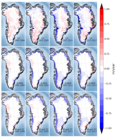
Figure 5.
(Upper panel) Surface elevation change of the Greenland ice sheet from radar altimetry. (Middle panel) Change in surface mass balance with respect to the reference period (1982–1992). (Lower panel) Change in volume as modelled by PISM when forcing PISM with HIRHAM5 surface mass balance and temperature.
The observations show an initial small increase in elevation over much of the ice sheet in the early part of the record but over the full period there has been an absolute decline in surface elevation, demonstrating the importance of long-term observations. There are some exceptions in the east and south where the trend to overall decrease in elevation is reversed through the period of observations. The decrease in surface elevation is particularly marked around the margins of the ice sheet [71] especially on the western side and around the basins of significant active calving glaciers, for example Jakobshavn Isbrae in the west and Helheim and Kangerlussuaq glacier basins in the east where surface elevation changes greater than 1 m per year are observed. In these locations, ice dynamics from fast flowing glaciers (see Figure 1) are likely to contribute to significant elevation change. Comparison between the SEC observed from radar altimetry (upper panel) with the modelled SMB (middle panel) and modelled SEC from the ISM (lower panel) suggests that surface mass processes of precipitation and melt dominate the observed SEC over the vast majority of the interior of the ice sheet. This supports analysis by [7] who also found SMB processes dominate the recent ice sheet mass budget. Around the margins of the ice sheet the modelled SMB from the RCM and SEC observations show a similar pattern of elevation change both in sign and in spatial extent. However, it is also noteworthy that the majority of the ice sheet interior shows a small surface increase in all four periods from observations; this is not reflected in the modelled SMB model, where the RCM may have a dry precipitation bias [5]. The observed surface elevation increase in this region may also result either from biases in the correction of snow density or from ice sheet dynamic processes related to colder, stiffer glacial period ice, as suggested by Colgan et al. [72]. The ice sheet dynamical model also does not capture this surface increase, though this may be due to uncertainties in the initialisation of the model as shown by Adalgeirsdottir et al. [14].
In the regions of fast flowing outlet glaciers that show a surface lowering much greater than derived from the SMB modelling, the role of ice dynamics is likely to be much more important. However, while the PISM model results also show the strong influence of the surface mass balance forcing from HIRHAM the match between model surface elevation change and observed in some of these regions is less apparent. The ice sheet model under-predicts the SEC in some of these areas and in some cases even has the wrong sign, for example at the terminus of Jakobshavn glacier. This is likely to be at least in part a result of the model resolution inadequately capturing basal topography [65] though may also reflect process parameter uncertainty that gives lower ice sheet velocities than observed in some locations as discussed in the following section. The lack of a dynamic calving parameterisation, a long-standing problem in ice sheet modelling [27], may also contribute to this underestimate in SEC as the model underestimates the increase in ice velocity gradients that lead to dynamic thinning [73] as calving rates increase. Work by [74] also indicates that increased basal and frontal melting at outlet glaciers can lead to enhanced dynamic thinning at glaciers with termini grounded in deep water. This process is not yet included in the PISM ice sheet model version used in this study and may thus also explain the mismatch between elevation change from the model and the satellite observations.
3.2. Modelled and Observed Ice Velocities
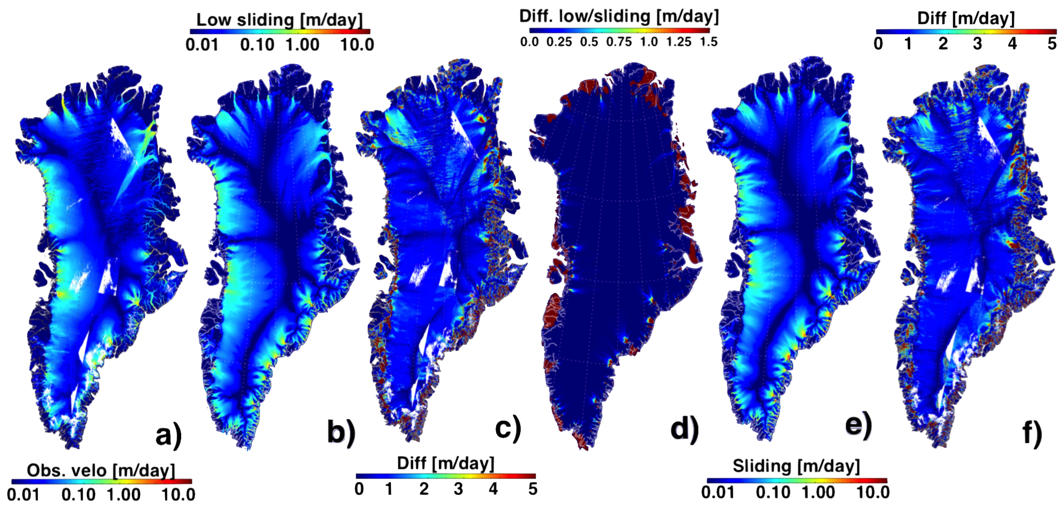
In ice sheet models, numerous parameters influence the observed dynamics of the ice and comparisons between observations and model results may assist in constraining model parameters. As an example, the effect of different sliding parameters on ice velocities have been examined. In Figure 6 the mean modelled ice velocities for the winter 2014–2015 (Oct–Mar) are compared to the corresponding observed ice velocity. Figure 6b shows the results for the low sliding case, while Figure 6e shows the enhanced sliding case. In both cases, overall structure of the flow field looks reasonable, even though the modelled velocities are too low. Ice streams are mostly properly located, even though the North Eastern Greenland Ice Stream (NEGIS) is less well represented. This is, however, a consistent feature of many ice sheet models since NEGIS dynamics are believed to be heavily influenced by geothermal heat anomalies [75,76,77] an effect that is currently not well accounted for in this model setup. One solution is to do an inversion with the model based on surface velocities to obtain basal friction, and then use this for the simulations. However, as it requires a consistent surface velocity covering the entire Greenland ice sheet, not just a single area, it would then be difficult to use the surface velocities as independent validation of the ice sheet model and is beyond the scope of this current study. In this set of experiments, PISM’s ice streams are generated by bedrock topography and a combination of sliding over the base and shear deformation of a thin till and ice layer at the base [60]. When sliding is included, see Figure 6e, the overall ice velocity increases and the individual ice streams become more focused. Figure 6d shows the difference in the modelled velocities. From the difference plot it is evident that the overall velocity of the ice changes very little in the two cases, but the velocity in the ice streams increases significantly and focuses the flow. Using the ice velocity data to tune the sliding enhancement factor provides a better correspondence with the observed ice velocities.
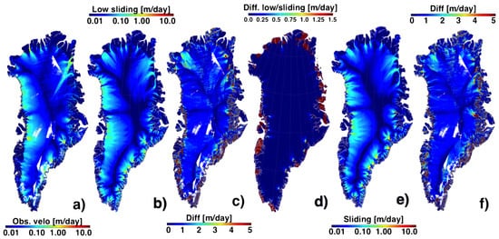
Figure 6.
Ice surface velocity in the winter of 2014–2015 (Oct–Mar). (a) Mean observed ice velocity. (b) Modelled ice velocity in the case of low sliding. (c) Difference in observed and low sliding model velocity (a vs. b). (d) The difference between the modelled ice velocities. (e) Modelled ice velocity with sliding included. (f) Difference in observed and sliding included model velocity (a vs. e).
3.3. Total Ice Sheet Mass Budget down to the Basin Scale
As Figure 4 showed, there has been a long-term downward trend in the total mass budget of the Greenland ice sheet, at least since the start of the GRACE era. The methods of Barletta et al. [41] and Groh and Horwath [42] applied to the GMB data give an average mass loss of 255 and 260 ± 15 Gt year respectively, though the contribution of each basin to this figure varies considerably. The GMB data can be used to determine how much of the mass loss is related to surface processes and how much to ice dynamics but it can also be used to assess how different models represent mass budget processes.
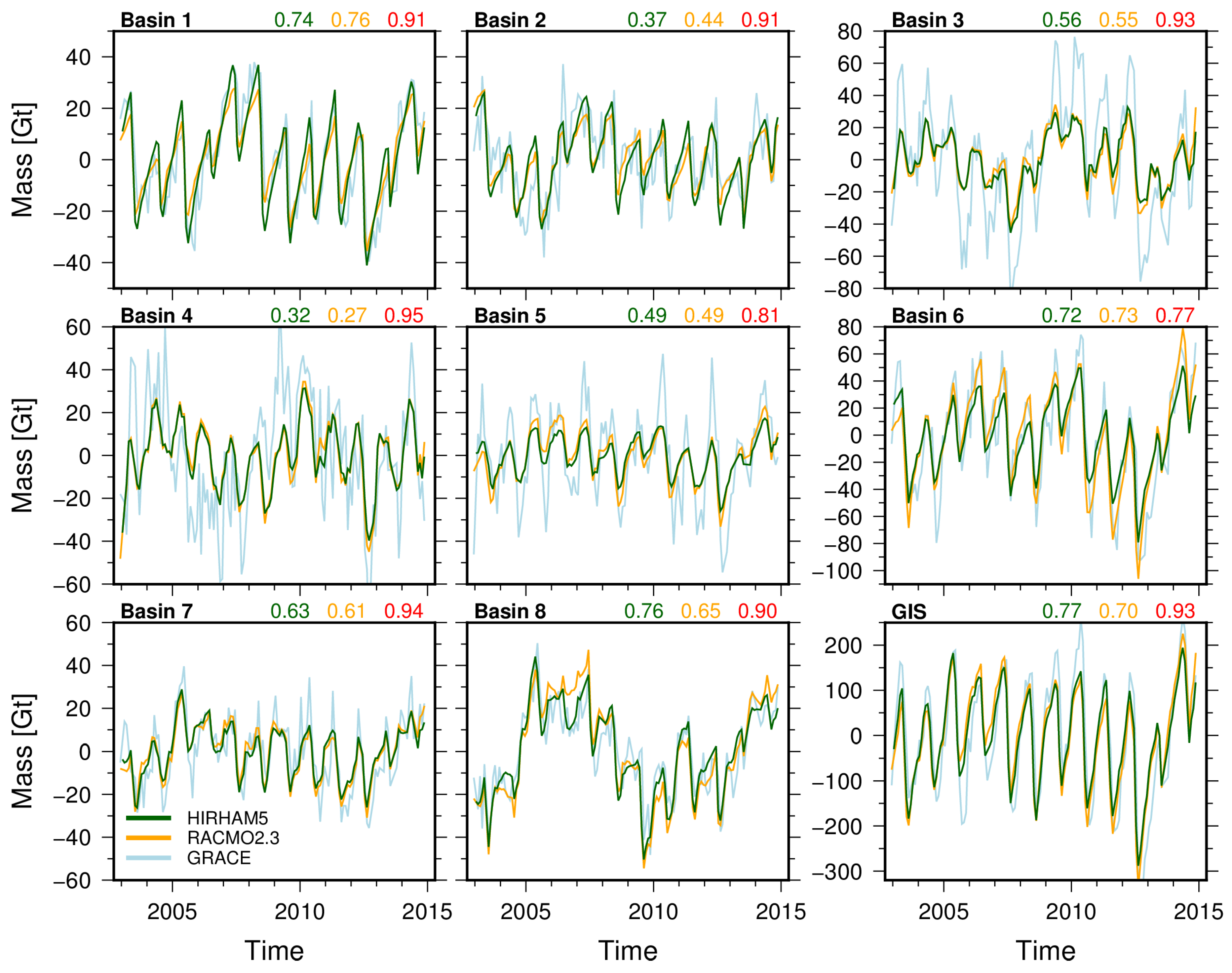
To compare surface mass changes modelled by HIRHAM5 and RACMO2.3 [10] with those observed by GRACE, cumulative SMB anomalies are calculated from the monthly SMB values of both models. Long-term signal components are removed by calculating residuals with regard to a linear model (for the SMB) and a quadratic (for the GMB) model. In this way, the impact of differing reference periods used for deriving the cumulative SMB anomalies and of ice-dynamical mass changes included in the GMB products are largely removed. Figure 7 compares residual mass changes for eight drainage basins and the whole Greenland ice sheet. The Nash-Sutcliffe model efficiency coefficient indicates the level of agreement between the GMB products and the model predictions as well as between both models.
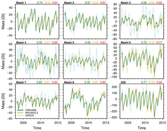
Figure 7.
Intercomparison of mass changes from GRACE (Greenland ice sheet CCI GMB product) and two regional climate models (HIRHAM5 and RACMO2.3) for different drainage basins (cf. inset in Figure 4) and the entire Greenland ice sheet. Mass changes are given w.r.t. a linear and quadratic model and exclude the long-term signal. Numbers indicate the Nash-Sutcliffe model efficiency coefficients for: GRACE vs. HIRHAM5 (green), GRACE vs. RACMO2.3 (orange) and HIRHAM5 vs. RACMO2.3 (red).
It is important to emphasise that there are uncertainties in the GRACE-derived estimates [78], e.g., caused by errors in the GRACE monthly solutions or by signal leakage from adjacent regions, as well as uncertainties in the SMB estimates [5,47] and seasonal fluctuations in ice dynamics [79]. These uncertainties complicate interpretation of the data. As the GMB data also accounts for ice dynamics, we would not necessarily expect a good agreement between modelled SMB and GMB data, especially in basins with high ice velocities and active calving fronts but in other basins a closer match between SMB and GMB should be expected. Overall there is good agreement between models and the GMB data for the ice sheet as a whole with some interesting regional variations as the statistics in Figure 7 confirm. The higher amplitude positive mass balance from GRACE in basins 3, 4 and 5 in eastern, south eastern and southern Greenland respectively, coincide with regions showing the highest precipitation inputs in Greenland. This suggests that the distribution of precipitation over the ice sheet is a significant source of uncertainty in both models and in terms of decomposing the GRACE land and ice signals. However, the high amplitude mass loss in the GRACE signal compared to the RCM data is especially apparent in basins 3, 4 and 5. These basins have large calving outlet glaciers and the GRACE data therefore suggests that glacier dynamics and ocean driven processes are enhancing mass loss in these regions. Basin 4 in southeast Greenland in particular has a large number of actively calving glaciers. The large mass loss recorded by the GMB from GRACE but not in the RCMs from 2005 to 2008 coincides with a period of retreat and active calving discussed further below.
The low surface elevation change calculated from the SMB model compared with the observed surface elevation change in the high interior of the ice sheet indicated that modelled precipitation from RCMs may be biased low over much of the interior. There is relatively little observational data for accumulation rates across Greenland. Analysis of field data collected along the Q-transect (the Qasimiut ice lobe) in southern Greenland [53], one of the few consistent time series of observations of accumulation, demonstrates that in basin 5, both RACMO and HIRHAM5 regional climate models overestimate precipitation over the ice sheet close to the margin and underestimate precipitation further inland as a result of the bias. Hermann et al. [53] point out that the precipitation bias has a consequent impact on the modelled melt rate. Melt at the surface of glaciers is strongly determined by the albedo. Snow has a higher albedo than bare glacier ice so the acceleration in melting that occurs when ice is exposed occurs later in the season in the models compared to the observations. The overestimate of snowfall from the models in this location leads to an underestimate in snow and ice melt during the melt season compared to that observed at stake sites on the glacier. The bias in mass loss in the RCMs compared to the GMB in this region may thus be partly explained by biases in precipitation as well as ice dynamic processes in basin 5. As some of the highest melt rates and highest snowfall rates have been recorded by automatic weather stations on the ice sheet in Greenland in basin 5, analysis of local effects as in Hermann et al. [53], also demonstrates the value in supplementing satellite based observations and models with field measurement campaigns.
Interestingly, in basins 1 and 2, where calving and ice dynamics are not as large contributors to mass loss as in other regions, modelled SMB and GMB data products match rather well. However, there are some significant differences between the two RCMs in some years in these regions as well as in region 8 in northwestern Greenland. We hypothesise that some of the variation between modelled SMB is due to the albedo effect and differing albedo parameterisations as well as perhaps different precipitation rates in the two models in these locations as documented in Noel et al. [10]. Northern Greenland has low precipitation rates and once darker glacier ice is exposed after fresh snow with a higher albedo melts away, large amounts of ice can be lost [80]. A small difference in precipitation in one model compared to the other, or different albedo parametrisations that substantially vary melt and runoff between the models, can thus have a large impact in these two basins. Differences in cloud parameterisations may well also result in a similar effect [11]. The regional scale analysis here also demonstrates that during the high mass loss year of 2012, around 25% of the mass loss came from basin 6 in western Greenland, driven by high melt rates. An underestimate in melt rates in HIRHAM5, and likely in other RCMs, particularly in the region of basin 6 during the heat wave of 2012 was identified by Fausto et al. [81] who compared weather station data on the ice sheet from the PROMICE network with model output. Their analysis suggested that this underestimate resulted from a bias in roughness lengths leading to underestimates of sensible and latent heat fluxes. Conversely, analysis by [82] showed relatively consistent and reliable performance by several different SMB models including HIRHAM and RACMO at a field site within this basin, suggesting that local factors can significantly influence model performance. Our analysis thus shows the value of detailed observations of mass change from field and satellite observations in interpreting and improving process understanding in Greenland and points to areas where the physical processes within regional climate modelled SMB need to be improved.
3.4. Calving Front Location and Ice Sheet Mass Budget
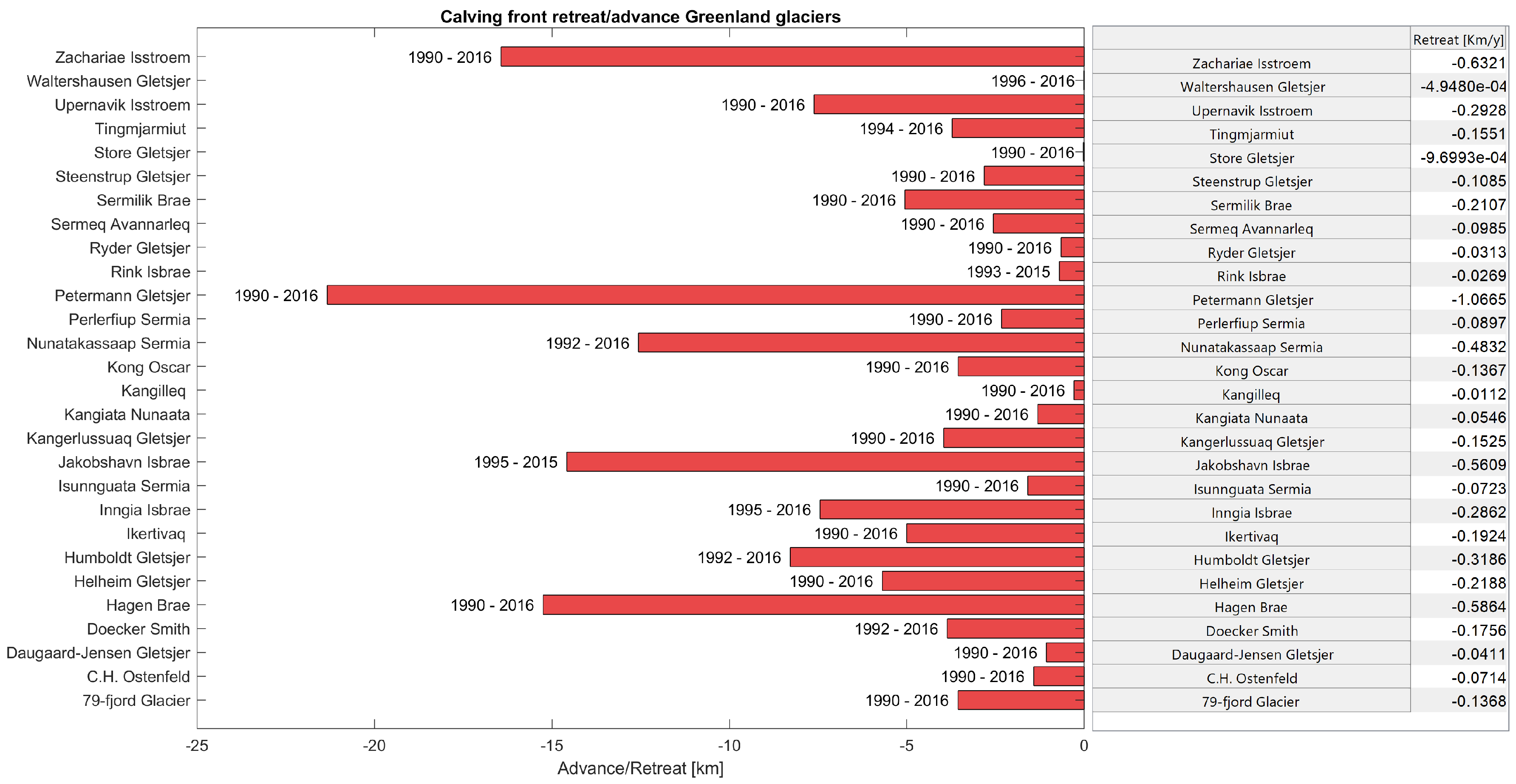
As the analysis of the GMB data compared with RCM data in Figure 7 shows, calving and ice-ocean interactions are an important component of the Greenland ice sheet mass budget. Since the start of the ESA-CCI project, outlet glacier retreat rates and associated increased calving rates have been a significant contribution to the observed mass loss from the Greenland ice sheet. Ref. [1,7,47] suggest that around one third of ice lost from the Greenland ice sheet is the result of iceberg calving and related processes. Out of the 28 glaciers monitored by the CCI project, all except two underwent significant retreat during the period 1990 to 2016 (Figure 8), though at very different rates when averaged over the long term. The time series in the calving front location (CFL) dataset are at least 20 years and in some cases almost 30 years suggesting that the consistent retreat of glaciers observed around Greenland is the result of widespread climate change in the region. While the 28 study glaciers are only a small sample, the pattern of calving front retreat is consistent with the other datasets we discuss here and with other studies in the literature (for example, [79]) and shows that the Greenland ice sheet is retreating both due to increased melt and runoff and due to dynamically controlled and ocean driven processes.
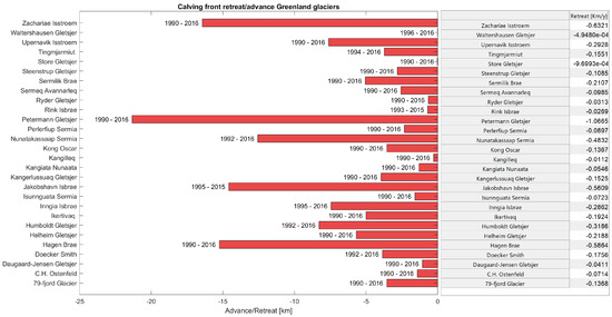
Figure 8.
Total calving front change for each of 28 outlet glaciers between the 1990s and 2016 (left). Each is given as the 2016 position minus the initial position. The annually averaged rate of position change over the period is given in the table (right).
As calving rates and calving front location are controlled by multiple processes (see below and also [27]), the total location change and retreat rate are sensitive to the start and end dates chosen. As Figure 9 shows, CFL is often at a stable position for a decade or longer, before a calving retreat that leads to a rapid change in position before establishing a new stable location. At Petermann glacier for example, the CFL gradually moves forward before a single calving event shortened the ice shelf dramatically, after which the CFL again started to move forward again. The normally episodic nature of changes in CFL emphasises the need for long-term monitoring to understand the behaviour of calving fronts and distinguish if retreat is within the bounds of natural variability or due to an external climate change forcing.
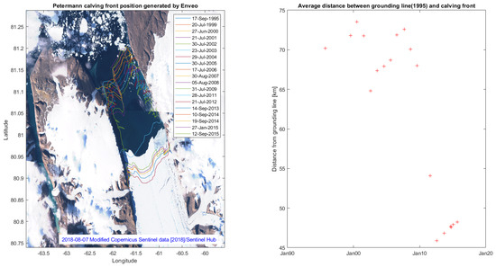
Figure 9.
(left) Petermann glacier calving front location between 1995 and 2015. (right) Average distance between a reference grounding line of 1995 and the calving front of Petermann glacier.
Significant outstanding research questions on calving outlet glaciers include how much of an influence surface and submarine melting of the glacier front have on calving front positions and the implementation of calving physics in ice sheet models. This is not a trivial problem and often relies on overly simplified empirical functions [73]. New process models, however, are now capable of detailed understanding of the key processes and are helping to improve calving laws [83] but as [84] show, substantial uncertainty around the rate and magnitude of future mass loss from the Greenland ice sheet due to calving will persist in the next round of the coupled model intercomparison project (CMIP6). The CFL dataset therefore presents significant possibilities for future work parameterising and evaluating calving losses from ice sheet models.
Most of the calving outlet glaciers in Greenland are tidewater type, that is with usually only a short and transiently floating calving front [27]. However, floating ice shelves similar to those found in Antarctica do exist in Greenland although typically confined within fjords [85]. During the course of the CCI project 2 of the 5 remaining floating ice shelves, Hagen Bræ and Zachariæ Isstrøm had significant retreat rates leaving only Petermann, Ryder and 79 glaciers with large and intact floating ice shelves at the present day. These glaciers with floating ice shelves are significant because each of these glaciers drain relatively large proportions of the ice sheet. The break-up of ice shelves that stabilise the outlet glaciers can lead to accelerations in ice velocity and therefore higher rates of sea level rise [29], but different glaciers respond in different ways to changes at the front [86] and careful modelling studies in combination with good observational data are required to understand the important processes [87]. For example, Rathmann et al. [21] showed different seasonal accelerations at neighbouring glaciers Zachariæ Isstrøm and 79 glacier in response to very similar runoff rates. Part of the differences were explained by different hydrological regimes but there is also a possibility that response to a climate forcing may be delayed by other glaciological processes such as differing bed topographies, geothermal heat flux or past strain histories. Similarly, Hogg et al. [16] showed that the grounding line at Petermann glacier has been mostly stable over the last half decade suggesting that the glacier is likely in equilibrium with the present day climate. However, more recently Rückamp et al. [88] showed an important link between calving retreat and increases in ice velocity at Petermann glacier as well as a retreat in the grounding line location, suggesting that longer time series of data are important to assess stability of ice shelves. By combining multiple datasets including the ice velocity, grounding line and calving front location with modelled surface runoff and an ice fracture model Rosier et al. [89], in review assess how stable the Petermann glacier ice shelf actually is (Figure 9). We here give a short overview as a case study in using multiple data types to gain insight into glacier processes.
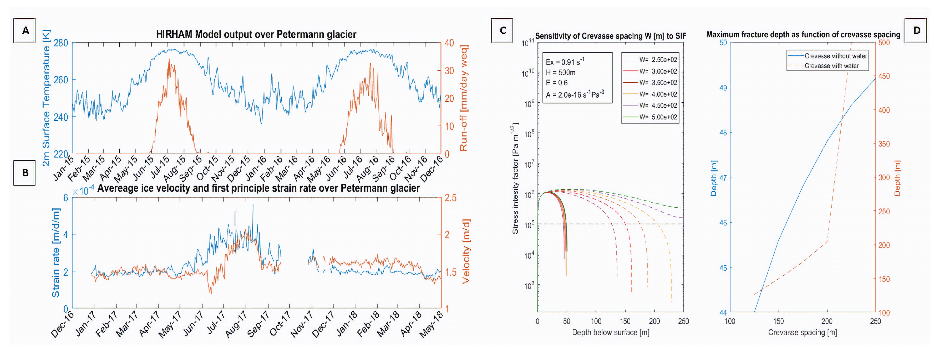
Analysis of the ice velocity dataset shows that velocity increases significantly in summer, likely due to melt water at the bed of the grounded part of Petermann glacier, reducing the basal pressure (Figure 10A). Increasing melt and runoff due to climate warming is therefore a plausible mechanism that can lead to increased calving and retreat of the calving fronts. Ice velocity data is used to derive strain rates that are further used to calculate crevasse penetration depths as described in [90] (Figure 10B). Crevasse depth models have been implemented as a parameterisation in ice sheet models to determine calving front location and the associated dynamic feedbacks by, for example Nick et al. [73]. The CCI ice velocity data products are therefore an ideal opportunity to derive strain rates and constrain estimates of calving activity.
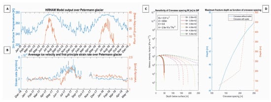
Figure 10.
(A) HIRHAM modelled 2-m temperature (blue) and run-off (orange) averaged over the Petermann glacier. (B) Sentinel-1 ice velocity (orange) and first principle strain rate (blue) averaged over the Petermann glacier. (C) Stress intensity factor at different depths for varying crevasse spacing. Solid lines correspond to dry crevasses. Dashed lines to crevasses with a water level of 10 m below the surface. (D) Depth a crevasse reaches when the stress intensity factor equals the fracture toughness. Dry crevasses (blue), water filled crevasses (orange).
Using Glen’s flow law [91] the principle stresses are calculated from the strain rates. We then apply a linear elastic fracture mechanics formulation to calculate the penetration depth of a crevasse for the given tensile stress based on [90,92]. Apart from the internal stresses, the maximum depth of a crevasse, and therefore whether calving can also occur is also controlled by the spacing between crevasses and the presence of water in crevasses as shown in Figure 10C,D. The stress intensity factor (shown in Figure 10C) is a quantitative measure that shows the stress state of a fracture considering the applied loading and fracture geometry. When the stress intensity factor reaches an empirically derived threshold known as fracture toughness, the fracture is considered unstable allowing it to propagate the entire thickness of the ice shelf rapidly. In Figure 10 we use a value of 100 MPa for the fracture toughness, based on analysis by [90]. Fracture spacing, W, is important in this analysis. The closer spaced crevasses (W < 400m) penetrate to shallower depths whereas the more widely spaced crevasses (W > 450m) lead to unstable propagation through the full ice shelf thickness. The presence of water in crevasses enhances crevasse penetration and can lead to fractures propagating through the entire thickness of the ice sheet [27,90]. At Petermann glacier in northern Greenland, liquid water in crevasses is present only during the summer months when there is liquid run-off present, nonetheless as Figure 10D shows even closely spaced crevasses filled with water can penetrate the full ice shelf thickness and at lower strain rates than dry crevasses. The sensitivity of the fracture depth to water suggests that under a warming climate with greater melt water production at the surface, the ice shelf may well be vulnerable to break up as other glaciers in this region have also collapsed, for example, the retreat at C.H. Ostenfeldt glacier shown in Figure 8 and described along with other Greenland glaciers by Hill et al. [85].
It follows that with increasing air temperatures, a higher density of lakes can form increasing the volume of water available for hydro fracturing and causing an increase in the ice tongue instability. However, this effect can be mitigated by drainage of excess water through surface rivers and basal channels [93,94]. Figure 10 therefore only shows the potential effect increasing runoff can have on the stability of the Petermann ice shelf. Equally, higher velocities, leading to higher strain rates could lead to deeper fractures, though this effect is reduced if more crevasses open since the crevasse spacing also affects the depth of an individual fracture. The final fracture depth is dependent on the ice thickness by the ratio of crevasse depth over ice thickness. A thicker ice shelf means that the ratio is smaller and, all other things considered equal, would reduce the final fracture depth. This is however only the case in the situation where there is enough water available for hydro fracturing, in the case that no water is present the final fracture depth would increase slightly relative to the thinner ice shelf. As [95] showed that basal melting is also important at Petermann glacier in reducing ice shelf thickness, ocean forcing that increases basal melt rates may at least initially and somewhat paradoxically help to stabilise fracture propagation via the geometric effect.
Regional climate change projections for example, [45,56], show a significant increase in melt water runoff across Greenland under two different climate change scenarios, particularly in northern Greenland. This indicates that floating ice shelves like Petermann glacier are vulnerable to future retreat, a conclusion supported by Nick et al. [86] and a possible explanation for the loss of the other ice shelves around Greenland. Extending this analysis at Petermann glacier to other outlet glaciers covered by the CCI Greenland ice sheet datasets could also give a wider indication of the potential stability of outlet glaciers. As the analysis of the GMB data in Figure 7 shows, calving and submarine processes are likely to be very important mass budget components in basins 3 and 4 in particular and to a lesser extent basins 5 and 7.
4. Outlook
In this review paper we have given an overview of the current mass budget of the Greenland ice sheet based on models and remote sensing observations. As Figure 4 clearly shows the total mass of the ice sheet has consistently declined over the GRACE period. Combining observations and models demonstrates that both surface mass balance processes and ice dynamics, including calving processes and ocean interactions are contributing to this mass loss. The ESA CCI Greenland Ice Sheet observational datasets have proved to be a powerful tool in understanding and improving estimates of ice sheet mass budget and the contribution to sea level rise as well as pinpointing areas where process understanding needs to be improved. The continuation of the generated datasets in the future and extension back in time where possible using data from older sensors is planned as part of the CCI+ project due to commence in 2019. The existing data products will be enhanced with an ice mass flux and discharge data set that combines remote sensing and model data to give a continually updated reconciled Greenland ice sheet mass budget as used, for example, in [2]. The successful launch of GRACE Follow-On (GRACE-FO) in May 2018 will also extend the time series of ice sheet total mass balance and allow for better assessments of regional variability. Similarly, continuing advances in the development of the next generation of RCMs such as the non-hydrostatic model HARMONIE-AROME already used for very high resolution (2.5 km) operational weather modelling in Greenland will help to improve estimates of SMB [12,96]. The development of new climate reanalysis such as MERRA-2 replay analyses and the Copernicus Arctic Reanalysis currently in production have great potential to derive more accurate SMB reconstructions and will also help to reduce process uncertainty. The analysis in this paper also demonstrates the value of on ice sheet observations from weather stations and stake measurements of surface mass balance [53]. Interpreting the mismatch between satellite data and model output is greatly assisted by the presence of reliable field data and thus helps to develop the science of ice sheet change further.
Our analysis of the variability within and between datasets also points to the importance of further improving models of surface mass balance, particularly with respect to precipitation and accumulation rates. Similarly, enhanced understanding and parameterisation of ice-ocean interactions will improve estimates of future sea level rise from Greenland.
5. Conclusions
The Greenland ice sheet has now been observed by satellite and documented in detail for almost three decades. The wealth of detailed information processed and made freely by the ESA climate change initiative has contributed to and will continue to contribute to significant advances in understanding processes of ice sheet change. In this study we summarise the present state of the mass budget of the Greenland ice sheet and the relative contributions from different processes.
Over the period 2003–2016 we find a gravimetric mass balance derived from GRACE for Greenland including the peripheral glaciers and ice caps of −255 ± 15 Gt year. Mass loss is driven mostly by surface mass balance processes though with a significant dynamical component in some ice sheet basins. After the significant acceleration in mass loss rate in the GRACE-era up to the record mass loss in the summer of 2012, Greenland has since seen a decrease in the short-term mass loss trend.
Combining data with models is a powerful way to enhance process understanding. Decomposing GMB into basins and comparing with RCM-derived SMB suggests models tend to overestimate precipitation over the ice sheet in some key basins and may also underestimate melt rates. At the same time, differences between RCM-derived SMB suggests that parameterisations within the models can lead to significant regional biases in mass budget estimates. Improved field data as well as improved parameterisations will help to solve some of these problems.
Surface elevation has reduced across almost all of the ice sheet with a small increase in elevation in the central highest altitude parts of the ice sheet. While RCMs mostly agree with the broad trends in SEC, the inability of RCMs to reproduce the small increase in SEC in the interior and particularly in eastern Greenland suggests that precipitation is underestimated by RCMs and/or that ice dynamic processes are partly responsible.
Analysis of model simulations from both regional climate models and ice sheet models demonstrate that SMB is driving most of the elevation change in the interior and at the margins of the ice sheet. However, drainage basins with fast-moving outlet glaciers demonstrate significant dynamic drawdown related to ice discharge and potentially basal and frontal melting. Some of these basins are modelled adequately by the ice sheet model PISM used in this study. Other basins were not well represented in PISM suggesting that running high resolution models and developing and implementing dynamic feedbacks and ocean driven melting related to calving retreat are necessary for ice sheet models to be able to accurately simulate ice dynamics.
The active retreat followed by stabilisation of a number of calving outlets is well documented [7] and correlates with the dynamically derived SEC and with areas of relatively high velocity in the ice velocity dataset.
Analysis of grounding lines suggests that the few remaining ice shelves are currently relatively stable [16] but analysis of the strain distribution across the ice shelf points to the importance of strain rates and surface melt water in enhancing fracture propagation. Increases in melt and/or strain rates due to increases in velocity gradients in the future may therefore lead to increased instability and likely collapse of the remaining ice shelves around Greenland [97]. Other metrics of ice shelf state such as ice shelf thickness, areal extent of meltwater ponding and basal melt channelization may prove to be better indicators of ice shelf stability in Greenland, given the different topographic configurations found in Greenland compared to the generally better studied Antarctic ice shelves [94].
Continued independent validation and comparison, along with focused field work and enhanced modelling of calving and ice dynamics will lead to more accurate ECV products. All of the data products reported here indicate significant impact on and response of the Greenland ice sheet to climate change. This allows us to define the current changes in Greenland as a baseline for the important processes likely to drive future ice sheet change and consequent sea level rise.
Supplementary Materials
Data Availability: All ESA CCI data products are available from the CCI data portal. http://esa-icesheets-greenland-cci.org/. HIRHAM5 regional climate model simulation data can be downloaded from the link given here: http://polarportal.dk/en/groenlands-indlandsis/nbsp/links/.
Author Contributions
R.M. and S.B.S. conceived and designed the outline for the paper. R.M. ran the HIRHAM5 regional climate model and analysed the output. S.B.S. and L.S.S. derived altimetry results. A.G. and V.R.B. estimated the Mass Balance from GRACE with input from M.H. S.H.S. performed ice sheet model study and comparisons between ice sheet model output and observations. R.F. lead the ESA CCI project for the Greenland ice sheet. T.N. and J.W. derived the ice velocity results. J.R. and R.M. developed and ran the calving and ice fracture model. A.S. and C.S.H. contributed fruitful and enlightening discussions around data presented here. All authors contributed to writing the paper and analyzing the results.
Acknowledgments
The authors acknowledge the ESA Climate change initiative for the Greenland ice sheet funded via ESA-ESRIN contract number 4000104815/11/I-NB. A.G., S.B.S. and V.B. also acknowledge funding by the European Space Agency in the framework of the Sea Level Budget Closure CCI Project funded via ESA-ESRIN contract number 4000119910/17/I-NB. HIRHAM5 regional climate model simulations were carried out by R.M. as part of the ice2ice project, a European Research Council project under the European Community’s Seventh Framework Programme (FP7/ 2007-2013)/ ERC grant agreement 610055. Development of PISM is supported by NASA grant NNX17AG65G and NSF grants PLR-1603799 and PLR-1644277. We thank the research group at IMAU, University of Utrecht for the RACMO2.3 regional climate model output used in Section 3.3.
Conflicts of Interest
The authors declare no conflict of interest.
References
- Van den Broeke, M.R.; Enderlin, E.M.; Howat, I.M.; Kuipers Munneke, P.; Noël, B.P.Y.; van de Berg, W.J.; van Meijgaard, E.; Wouters, B. On the recent contribution of the Greenland ice sheet to sea level change. Cryosphere 2016, 10, 1933–1946. [Google Scholar] [CrossRef]
- Shepherd, A.; Ivins, E.R.; Geruo, A.; Barletta, V.R.; Bentley, M.J.; Bettadpur, S.; Briggs, K.H.; Bromwich, D.H.; Forsberg, R.; Galin, N.; et al. A Reconciled Estimate of Ice-Sheet Mass Balance. Science 2012, 338, 1183–1189. [Google Scholar] [CrossRef] [PubMed]
- Vaughan, D.G.; Comiso, J.C.; Allison, I.; Carrasco, J.; Kaser, G.; Kwok, R.; Mote, P.; Murray, T.; Paul, F.; Ren, J.; et al. Observations: Cryosphere. Clim. Chang. 2013, 2103, 317–382. [Google Scholar]
- Cappelen, J. Greenland-Dmi Historical Climate Data Collection 1784-2017; Danish Meteorological Institue Report 18-04; Danish Meteorological Institute: Copenhagen, Denmark, 2017. [Google Scholar]
- Langen, P.L.; Fausto, R.S.; Vandecrux, B.; Mottram, R.H.; Box, J.E. Liquid Water Flow and Retention on the Greenland Ice Sheet in the Regional Climate Model HIRHAM5: Local and Large-Scale Impacts. Front. Earth Sci. 2017, 4. [Google Scholar] [CrossRef]
- Rignot, E.; Fenty, I.; Xu, Y.; Cai, C.; Kemp, C. Undercutting of marine-terminating glaciers in West Greenland. Geophys. Res. Lett. 2015, 42, 5909–5917. [Google Scholar] [CrossRef] [PubMed]
- Enderlin, E.M.; Howat, I.M.; Jeong, S.; Noh, M.J.; Angelen, J.H.; Broeke, M.R. An improved mass budget for the Greenland ice sheet. Geophys. Res. Lett. 2014, 41, 866–872. [Google Scholar] [CrossRef]
- Akperov, M.; Rinke, A.; Mokhov, I.I.; Matthes, H.; Semenov, V.A.; Adakudlu, M.; Cassano, J.; Christensen, J.H.; Dembitskaya, M.A.; Dethloff, K.; et al. Cyclone Activity in the Arctic From an Ensemble of Regional Climate Models (Arctic CORDEX). J. Geophys. Res. Atmos. 2018, 123, 2537–2554. [Google Scholar] [CrossRef]
- Lucas-Picher, P.; Wulff-Nielsen, M.; Christensen, J.H.; Aðalgeirsdóttir, G.; Mottram, R.; Simonsen, S.B. Very high resolution regional climate model simulations over Greenland: Identifying added value: RCM SIMULATIONS FOR GREENLAND. J. Geophys. Res. Atmos. 2012, 117. [Google Scholar] [CrossRef]
- Noel, B.; van de Berg, W.; van Meijgaard, E.; Kuipers Munneke, P.; van de Wal, R.; van den Broeke, M. Evaluation of the updated regional climate model RACMO2.3: summer snowfall impact on the Greenland Ice Sheet. Cryosphere 2015, 9, 1831–1844. [Google Scholar] [CrossRef]
- Van Tricht, K.; Lhermitte, S.; Lenaerts, J.T.M.; Gorodetskaya, I.V.; L’Ecuyer, T.S.; Noël, B.; van den Broeke, M.R.; Turner, D.D.; van Lipzig, N.P.M. Clouds enhance Greenland ice sheet meltwater runoff. Nat. Commun. 2016, 7, 10266. [Google Scholar] [CrossRef]
- Mottram, R.; Nielsen, K.P.; Gleeson, E.; Yang, X. Modelling Glaciers in the HARMONIE-AROME NWP model. Adv. Sci. Res. 2017, 14, 323–334. [Google Scholar] [CrossRef][Green Version]
- Vernon, C.L.; Bamber, J.L.; Box, J.E.; van den Broeke, M.R.; Fettweis, X.; Hanna, E.; Huybrechts, P. Surface mass balance model intercomparison for the Greenland ice sheet. Cryosphere 2013, 7, 599–614. [Google Scholar] [CrossRef]
- Adalgeirsdottir, G.; Aschwanden, A.; Khroulev, C.; Boberg, F.; Mottram, R.; Lucas-Picher, P.; Christensen, J.H. Role of model initialization for projections of 21st-century Greenland ice sheet mass loss. J. Glaciol. 2014, 60, 782–794. [Google Scholar] [CrossRef]
- Joughin, I.; Fahnestock, M.; Kwok, R.; Gogineni, P.; Allen, C. Ice flow of Humboldt, Petermann and Ryder Gletscher, northern Greenland. J. Glaciol. 1999, 45, 231–241. [Google Scholar] [CrossRef][Green Version]
- Hogg, A.E.; Shepherd, A.; Gourmelen, N.; Engdahl, M. Grounding line migration from 1992 to 2011 on Petermann Glacier, North-West Greenland. J. Glaciol. 2016, 62, 1104–1114. [Google Scholar] [CrossRef]
- Sørensen, L.S.; Simonsen, S.B.; Nielsen, K.; Lucas-Picher, P.; Spada, G.; Adalgeirsdottir, G.; Forsberg, R.; Hvidberg, C.S. Mass balance of the Greenland ice sheet (2003–2008) from ICESat data—The impact of interpolation, sampling and firn density. Cryosphere 2011, 5, 173–186. [Google Scholar] [CrossRef]
- Sørensen, L.S.; Simonsen, S.B.; Meister, R.; Forsberg, R.; Levinsen, J.F.; Flament, T. Envisat-derived elevation changes of the Greenland ice sheet, and a comparison with ICESat results in the accumulation area. Remote Sens. Environ. 2015, 160, 56–62. [Google Scholar] [CrossRef]
- Simonsen, S.B.; Sørensen, L.S. Implications of changing scattering properties on Greenland ice sheet volume change from Cryosat-2 altimetry. Remote Sens. Environ. 2017, 190, 207–216. [Google Scholar] [CrossRef]
- Sandberg Sørensen, L.; Simonsen, S.B.; Forsberg, R.; Khvorostovsky, K.; Meister, R.; Engdahl, M.E. 25 years of elevation changes of the Greenland Ice Sheet from ERS, Envisat, and CryoSat-2 radar altimetry. Earth Planet. Sci. Lett. 2018, 495, 234–241. [Google Scholar] [CrossRef]
- Rathmann, N.M.; Hvidberg, C.S.; Solgaard, A.M.; Grinsted, A.; Gudmundsson, G.H.; Langen, P.L.; Nielsen, K.P.; Kusk, A. Highly temporally resolved response to seasonal surface melt of the Zachariae and 79N outlet glaciers in northeast Greenland. Geophys. Res. Lett. 2017, 44, 9805–9814. [Google Scholar] [CrossRef]
- Nagler, T.; Rott, H.; Hetzenecker, M.; Wuite, J.; Potin, P. The Sentinel-1 Mission: New Opportunities for Ice Sheet Observations. Remote Sens. 2015, 7, 9371–9389. [Google Scholar] [CrossRef]
- Simonsen, S.B.; Stenseng, L.; Ađalgeirsdóttir, G.; Fausto, R.S.; Hvidberg, C.S.; Lucas-Picher, P. Assessing a multilayered dynamic firn-compaction model for Greenland with ASIRAS radar measurements. J. Glaciol. 2013, 59, 545–558. [Google Scholar] [CrossRef]
- Boncori, J.P.M.; Andersen, M.L.; Dall, J.; Kusk, A.; Kamstra, M.; Andersen, S.B.; Bechor, N.; Bevan, S.; Bignami, C.; Gourmelen, N.; et al. Intercomparison and Validation of SAR-Based Ice Velocity Measurement Techniques within the Greenland Ice Sheet CCI Project. Remote Sens. 2018, 10, 929. [Google Scholar] [CrossRef]
- Joughin, I. MEaSUREs Greenland Ice Sheet Velocity Map from InSAR Data, Version 2; National Snow and Ice Data Center: Boulder, CO, USA, 2015. [Google Scholar]
- Khvorostovsky, K. Algorithm Theoretical Baseline Document (ATBD) for the Greenland Ice Sheet CCI Project of ESA’s Climate Change Initiative, Version 3.2. Available online: http://esa-icesheets-greenland-cci.org/sites/default/files/documents/public/Phase (accessed on 30 May 2019).
- Benn, D.I.; Warren, C.R.; Mottram, R.H. Calving processes and the dynamics of calving glaciers. Earth-Sci. Rev. 2007, 82, 143–179. [Google Scholar] [CrossRef]
- Schoof, C. Ice sheet grounding line dynamics: Steady states, stability, and hysteresis. J. Geophys. Res. Earth Surf. 2007, 112. [Google Scholar] [CrossRef]
- Mouginot, J.; Rignot, E.; Scheuchl, B.; Fenty, I.; Khazendar, A.; Morlighem, M.; Buzzi, A.; Paden, J. Fast retreat of Zachariæ Isstrøm, northeast Greenland. Science 2015, 350, 1357–1361. [Google Scholar] [CrossRef] [PubMed]
- Rignot, E.; Velicogna, I.; van den Broeke, M.R.; Monaghan, A.; Lenaerts, J.T. Acceleration of the contribution of the Greenland and Antarctic ice sheets to sea level rise. Geophys. Res. Lett. 2011, 38. [Google Scholar] [CrossRef]
- Rignot, E.; Mouginot, J.; Scheuchl, B. Antarctic grounding line mapping from differential satellite radar interferometry: GROUNDING LINE OF ANTARCTICA. Geophys. Res. Lett. 2011, 38. [Google Scholar] [CrossRef]
- Nagler, T. Comprehensive Error Characterisation Report (CECR). Antarctic Ice Sheet cci project, ESA’s Climate Change Initiative, Version 3.0. 2018. Available online: http://esa-icesheets-antarctica-cci.org/index.php?q=webfm_send/84 (accessed on 30 May 2019).
- Davis, C.; Ferguson, A. Elevation change of the Antarctic ice sheet, 1995–2000, from ERS-2 satellite radar altimetry. IEEE Trans. Geosci. Remote Sens. 2004, 42, 2437–2445. [Google Scholar] [CrossRef]
- Johannessen, O.M. Recent Ice-Sheet Growth in the Interior of Greenland. Science 2005, 310, 1013–1016. [Google Scholar] [CrossRef]
- Khvorostovsky, K.S. Merging and Analysis of Elevation Time Series Over Greenland Ice Sheet From Satellite Radar Altimetry. IEEE Trans. Geosci. Remote Sens. 2012, 50, 23–36. [Google Scholar] [CrossRef]
- Levinsen, J.; Khvorostovsky, K.; Ticconi, F.; Shepherd, A.; Forsberg, R.; Sørensen, L.; Muir, A.; Pie, N.; Felikson, D.; Flament, T.; et al. ESA ice sheet CCI: derivation of the optimal method for surface elevation change detection of the Greenland ice sheet—Round robin results. Int. J. Remote Sens. 2015, 36, 551–573. [Google Scholar] [CrossRef]
- Tapley, B.; Bettadpur, S.; Watkins, M.; Reigber, C. The gravity recovery and climate experiment: Mission overview and early results. Geophys. Res. Lett. 2004, 31, L09607. [Google Scholar] [CrossRef]
- Mayer-Gürr, T.; Behzadpour, S.; Ellmer, M.; Kvas, A.; Klinger, B.; Zehentner, N. ITSG-Grace2016–Monthly and Daily Gravity Field Solutions from GRACE. GFZ Data Serv. 2016. [Google Scholar] [CrossRef]
- Bettadpur, S. UTCSR Level-2 Processing Standards Document for Level-2 Product Release 0006; Technical Report; University of Texas at Austin: Austin, TX, USA, 2018. [Google Scholar]
- Zwally, H.; Giovinetto, M.; Beckley, M.; Saba, J. Antarctic and Greenland Drainage Systems. Available online: http://icesat4.gsfc.nasa.gov/cryo_data/ant_grn_drainage_systems.php (accessed on 30 May 2019).
- Barletta, V.R.; Sørensen, L.S.; Forsberg, R. Scatter of mass changes estimates at basin scale for Greenland and Antarctica. Cryosphere 2013, 7, 1411–1432. [Google Scholar] [CrossRef]
- Groh, A.; Horwath, M. The method of tailored sensitivity kernels for GRACE mass change estimates. In Proceedings of the EGU General Assembly 2016, Vienna, Austria, 17–22 April 2016; Volume 18. [Google Scholar]
- Wahr, J.; Zhong, S. Computations of the viscoelastic response of a 3-D compressible Earth to surface loading: An application to Glacial Isostatic Adjustment in Antarctica and Canada. Geophys. J. Int. 2013, 192, 557–572. [Google Scholar] [CrossRef]
- Peltier, W.; Argus, D.; Drummond, R. Space geodesy constrains ice age terminal deglaciation: The global ICE-6G_C (VM5a) model: Global Glacial Isostatic Adjustment. J. Geophys. Res. Solid Earth 2015, 120, 450–487. [Google Scholar] [CrossRef]
- Mottram, R.; Boberg, F.; Langen, P.; Yang, S.; Rodehacke, C.; Christensen, J.H.; Madsen, M.S. Surface Mass balance of the Greenland ice Sheet in the Regional Climate Model HIRHAM5: Present State and Future Prospects. Low Temp. Sci. 2017, 75, 1–11. [Google Scholar] [CrossRef]
- Sasgen, I.; van den Broeke, M.; Bamber, J.; Rignot, E.; Sørensen, L.; Wouters, B.; Martinec, Z.; Velicogna, I.; Simonsen, S. Timing and origin of recent regional ice-mass loss in Greenland. Earth Planet. Sci. Lett. 2012, 333–334, 293–303. [Google Scholar] [CrossRef]
- Van den Broeke, M.; Bamber, J.; Ettema, J.; Rignot, E.; Schrama, E.; van de Berg, W.J.; van Meijgaard, E.; Velicogna, I.; Wouters, B. Partitioning Recent Greenland Mass Loss. Science 2009, 326, 984–986. [Google Scholar] [CrossRef]
- Dee, D.P.; Uppala, S.M.; Simmons, A.; Berrisford, P.; Poli, P.; Kobayashi, S.; Andrae, U.; Balmaseda, M.; Balsamo, G.; Bauer, D.P.; et al. The ERA-Interim reanalysis: Configuration and performance of the data assimilation system. Q. J. R. Meteorol. Soc. 2011, 137, 553–597. [Google Scholar] [CrossRef]
- Roeckner, E.; Oberhuber, J.M.; Bacher, A.; Christoph, M.; Kirchner, I. ENSO variability and atmospheric response in a global coupled atmosphere-ocean GCM. Clim. Dyn. 1996, 12, 737–754. [Google Scholar] [CrossRef]
- Rae, J.G.L.; Aðalgeirsdóttir, G.; Edwards, T.L.; Fettweis, X.; Gregory, J.M.; Hewitt, H.T.; Lowe, J.A.; Lucas-Picher, P.; Mottram, R.H.; Payne, A.J.; et al. Greenland ice sheet surface mass balance: Evaluating simulations and making projections with regional climate models. Cryosphere 2012, 6, 1275–1294. [Google Scholar] [CrossRef]
- Langen, P.L.; Mottram, R.H.; Christensen, J.H.; Boberg, F.; Rodehacke, C.B.; Stendel, M.; van As, D.; Ahlstrøm, A.P.; Mortensen, J.; Rysgaard, S.; et al. Quantifying Energy and Mass Fluxes Controlling Godthåbsfjord Freshwater Input in a 5-km Simulation (1991–2012). J. Clim. 2015, 28, 3694–3713. [Google Scholar] [CrossRef]
- Eerola, K. Twenty-one years of verification from the HIRLAM NWP system. Weather Forecast. 2013, 28, 270–285. [Google Scholar] [CrossRef]
- Hermann, M.; Box, J.E.; Fausto, R.S.; Colgan, W.T.; Langen, P.L.; Mottram, R.; Wuite, J.; Noël, B.; van den Broeke, M.R.; van As, D. Application of PROMICE Q-Transect in Situ Accumulation and Ablation Measurements (2000–2017) to Constrain Mass Balance at the Southern Tip of the Greenland Ice Sheet. J. Geophys. Res. Earth Surf. 2018, 123, 1235–1256. [Google Scholar] [CrossRef]
- Mote, T.L.; Anderson, M.R. Variations in snowpack melt on the Greenland ice sheet based on passive-microwave measurements. J. Glaciol. 1995, 41, 51–60. [Google Scholar] [CrossRef]
- Ettema, J.; van den Broeke, M.R.; van Meijgaard, E.; van de Berg, W.J.; Bamber, J.L.; Box, J.E.; Bales, R.C. Higher surface mass balance of the Greenland ice sheet revealed by high-resolution climate modeling. Geophys. Res. Lett. 2009, 36. [Google Scholar] [CrossRef]
- Fettweis, X.; Franco, B.; Tedesco, M.; van Angelen, J.H.; Lenaerts, J.T.M.; van den Broeke, M.R.; Gallae, H. Estimating the Greenland ice sheet surface mass balance contribution to future sea level rise using the regional atmospheric climate model MAR. Cryosphere 2013, 7, 469–489. [Google Scholar] [CrossRef]
- Vizcaino, M. Ice sheets as interactive components of Earth System Models: Progress and challenges. WIRES Clim. Chang. 2014, 5, 557–568. [Google Scholar] [CrossRef]
- Goelzer, H.; Robinson, A.; Seroussi, H.; van de Wal, R.S. Recent Progress in Greenland Ice Sheet Modelling. Curr. Clim. Chang. Rep. 2017, 3, 291–302. [Google Scholar] [CrossRef]
- Kirchner, N.; Hutter, K.; Jakobsson, M.; Gyllencreutz, R. Capabilities and limitations of numerical ice sheet models; a discussion for Earth-scientists and modelers. Q. Sci. Rev. 2011, 30, 3691–3704. [Google Scholar] [CrossRef]
- Bueler, E.; Brown, J.; Lingle, C. Exact solutions to the thermomechanically coupled shallow ice approximation: effective tools for verification. J. Glaciol. 2007, 53, 499–516. [Google Scholar] [CrossRef]
- Aschwanden, A.; Bueler, E.; Khroulev, C.; Blatter, H. An enthalpy formulation for glaciers and ice sheets. J. Glaciol. 2012, 58, 441–457. [Google Scholar] [CrossRef]
- Theoretical Glaciology: Mateial Science of Ice and the Mechanics of Glaciers and Ice Sheets; Number 1 in Mathematical Approaches to Geophysics; Springer: Berlin/Heidelberg, Germany, 1983.
- Morland, L. Plane and Radial Ice-Shelf Flow with Prescirpbed Temperature Profile. In Dynamics of the West Antarctic Ice Sheet; van der Veen, C.J., Oelemans, J., Eds.; D. Reidel Publishing Company: Dordrecht, The Netherlands, 1987. [Google Scholar]
- Bueler, E.; Brown, J. Shallow shelf approximation as a “sliding law” in a thermomechanically coupled ice sheet model. J. Geophys. Res. Earth Surf. 2009, 114. [Google Scholar] [CrossRef]
- Aschwanden, A.; Fahnestock, M.A.; Truffer, M. Complex Greenland outlet glacier flow captured. Nat. Commun. 2016, 7, 10524. [Google Scholar] [CrossRef]
- Khroulev, C.; PISM Authors. PISM, a Parallel Ice Sheet Model: User’s Manual. Available online: http://pism-docs.org/wiki/lib/exe/fetch.php?media=pism_manual.pdf (accessed on 31 May 2019).
- Bamber, J.; Layberry, R.; Gogenini, S. A new ice thickness and bed data set for the Greenland ice sheet1: Measurement, data reduction, and errors. J. Geophys. Res. 2001, 106, 33773–33780. [Google Scholar] [CrossRef]
- Nowicki, S.; Bindschadler, R.A.; Abe-Ouchi, A.; Aschwanden, A.; Bueler, E.; Choi, H.; Fastook, J.; Granzow, G.; Greve, R.; Gutowski, G.; et al. Insight into spatial sensitivities of ice mass response to environmental change from the SeaRISE ice sheet modeling project II: Greenland. J. Geophys. Res. 2013, 118, 1025–1044. [Google Scholar] [CrossRef]
- Velicogna, I.; Wahr, J. Acceleration of Greenland ice mass loss in spring 2004. Nature 2006, 443, 329–331. [Google Scholar] [CrossRef]
- Svendsen, P.; Andersen, O.; Nielsen, A. Acceleration of the Greenland ice sheet mass loss as observed by GRACE: Confidence and sensitivity. Earth Planet. Sci. Lett. 2013, 364, 24–29. [Google Scholar] [CrossRef]
- Krabill, W.; Hanna, E.; Huybrechts, P.; Abdalati, W.; Cappelen, J.; Csatho, B.; Frederick, E.; Manizade, S.; Martin, C.; Sonntag, J.; et al. Greenland Ice Sheet: Increased coastal thinning. Geophys. Res. Lett. 2004, 31. [Google Scholar] [CrossRef]
- Colgan, W.; Rajaram, H.; Abdalati, W.; McCutchan, C.; Mottram, R.; Moussavi, M.S.; Grigsby, S. Glacier crevasses: Observations, models, and mass balance implications: Glacier Crevasses. Rev. Geophys. 2016, 54, 119–161. [Google Scholar] [CrossRef]
- Nick, F.; Van Der Veen, C.; Vieli, A.; Benn, D. A physically based calving model applied to marine outlet glaciers and implications for the glacier dynamics. J. Glaciol. 2010, 56, 781–794. [Google Scholar] [CrossRef]
- Porter, D.F.; Tinto, K.J.; Boghosian, A.L.; Csatho, B.M.; Bell, R.E.; Cochran, J.R. Identifying Spatial Variability in Greenland’s Outlet Glacier Response to Ocean Heat. Front. Earth Sci. 2018, 6, 90. [Google Scholar] [CrossRef]
- Fahnestock, M.; Abdalati, W.; Joughin, I.; Brozena, J.; Gogineni, P. High Geothermal Heat Flow, Basal Melt, and the Origin of Rapid Ice Flow in Central Greenland. Science 2001, 294, 2338–2342. [Google Scholar] [CrossRef]
- Christanson, K.; Peters, L.E.; Alley, R.B.; Anandakrishnan, S.; Jacobel, R.W.; Riverman, K.L.; Muto, A.; Keisling, B.A. Dilatant till facilitates ice-stream flow in northeast Greenland. Earth Planet. Sci. Lett. 2014, 401, 57–69. [Google Scholar] [CrossRef]
- Rogozhina, I.; Petrunin, A.G.; Vaughan, A.P.; Steinberger, B.; Johnson, J.V.; Kaban, M.K.; Reinhard, C.; Rickers, F.; Thomas, M.; Koulakov, I. Melting at the base of the Greenland ice sheet explained by Iceland hotspot history. Nat. Geosci. 2016, 9, 366–369. [Google Scholar] [CrossRef]
- Wahr, J.; Swenson, S.; Velicogna, I. Accuracy of GRACE mass estimates. Geophys. Res. Lett. 2006, 33. [Google Scholar] [CrossRef]
- Moon, T.; Joughin, I.; Smith, B. Seasonal to multiyear variability of glacier surface velocity, terminus position, and sea ice/ice mélange in northwest Greenland. J. Geophys. Res. Earth Surf. 2015, 120, 818–833. [Google Scholar] [CrossRef]
- Tedesco, M.; Doherty, S.; Fettweis, X.; Alexander, P.; Jeyaratnam, J.; Stroeve, J. The darkening of the Greenland ice sheet: trends, drivers, and projections (1981–2100). Cryosphere 2016, 10, 477–496. [Google Scholar] [CrossRef]
- Fausto, R.; van As, D.; Box, J.; Colgan, W.; Langen, P. Quantifying the surface energy fluxes in South Greenland during the 2012 high melt episodes using in-situ observations. Front. Earth Sci. 2016, 4, 82. [Google Scholar] [CrossRef]
- Smith, L.C.; Yang, K.; Pitcher, L.H.; Overstreet, B.T.; Chu, V.W.; Rennermalm, A.K.; Ryan, J.C.; Cooper, M.G.; Gleason, C.J.; Tedesco, M.; et al. Direct measurements of meltwater runoff on the Greenland ice sheet surface. Proc. Natl. Acad. Sci. USA 2017, 114, E10622–E10631. [Google Scholar] [CrossRef] [PubMed]
- Benn, D.I.; Cowton, T.; Todd, J.; Luckman, A. Glacier Calving in Greenland. Curr. Clim. Chang. Rep. 2017, 3, 282–290. [Google Scholar] [CrossRef]
- Goelzer, H.; Nowicki, S.; Edwards, T.; Beckley, M.; Abe-Ouchi, A.; Aschwanden, A.; Calov, R.; Gagliardini, O.; Gillet-Chaulet, F.; Golledge, N.R.; et al. Design and results of the ice sheet model initialisation experiments initMIP-Greenland: An ISMIP6 intercomparison. Cryosphere 2018, 12, 1433–1460. [Google Scholar] [CrossRef]
- Hill, E.A.; Carr, J.R.; Stokes, C.R.; Gudmundsson, G.H. Dynamic changes in outlet glaciers in northern Greenland from 1948 to 2015. Cryosphere 2018, 12, 3243–3263. [Google Scholar] [CrossRef]
- Nick, F.; Luckman, A.; Vieli, A.; Van Der Veen, C.; Van As, D.; Van De Wal, R.; Pattyn, F.; Hubbard, A.; Floricioiu, D. The response of Petermann Glacier, Greenland, to large calving events, and its future stability in the context of atmospheric and oceanic warming. J. Glaciol. 2012, 58, 229–239. [Google Scholar] [CrossRef]
- Morlighem, M.; Williams, C.N.; Rignot, E.; An, L.; Arndt, J.E.; Bamber, J.L.; Catania, G.; Chauché, N.; Dowdeswell, J.A.; Dorschel, B.; et al. BedMachine v3: Complete Bed Topography and Ocean Bathymetry Mapping of Greenland From Multibeam Echo Sounding Combined With Mass Conservation. Geophys. Res. Lett. 2017, 4, 11051–11061. [Google Scholar] [CrossRef]
- Rückamp, M.; Neckel, N.; Berger, S.; Humbert, A.; Helm, V. Calving Induced Speedup of Petermann Glacier. J. Geophys. Res. Earth Surf. 2019. [Google Scholar] [CrossRef]
- Rosier, J.; Mottram, R.; Lhermitte, S.; Hetzenecker, M. Channelised melting and fracturing provide early warning of petermann ice shelf collapse. Sci. Adv. 2019. under review. [Google Scholar]
- Mottram, R.H.; Benn, D.I. Testing crevasse-depth models: A field study at Breidamerkurjokull, Iceland. J. Glaciol. 2009, 55, 746–752. [Google Scholar] [CrossRef]
- Glen, J.W. The Creep of Polycrystalline Ice. Proc. R. Soc. A Math. Phys. Eng. Sci. 1955, 228, 519–538. [Google Scholar] [CrossRef]
- Van der Veen, C. Fracture mechanics approach to penetration of surface crevasses on glaciers. Cold Regions Sci. Technol. 1998, 27, 31–47. [Google Scholar] [CrossRef]
- MacDonald, G.; Banwell, A.; MacAyeal, D.R. Seasonal evolution of supraglacial lakes on a floating ice tongue, Petermann Glacier, Greenland. Ann. Glaciol. 2018, 1–10. [Google Scholar] [CrossRef]
- Dow, C.F.; Lee, W.S.; Greenbaum, J.S.; Greene, C.A.; Blankenship, D.D.; Poinar, K.; Forrest, A.L.; Young, D.A.; Zappa, C.J. Basal channels drive active surface hydrology and transverse ice shelf fracture. Sci. Adv. 2018, 4, eaao7212. [Google Scholar] [CrossRef] [PubMed]
- Rignot, E.; Steffen, K. Channelized bottom melting and stability of floating ice shelves. Geophys. Res. Lett. 2008, 35. [Google Scholar] [CrossRef]
- Bengtsson, L.; Andrae, U.; Aspelien, T.; Batrak, Y.; Calvo, J.; de Rooy, W.; Gleeson, E.; Hansen-Sass, B.; Homleid, M.; Hortal, M.; et al. The HARMONIE—AROME Model Configuration in the ALADIN–HIRLAM NWP System. Mon. Weather Rev. 2017, 145, 1919–1935. [Google Scholar] [CrossRef]
- Münchow, A.; Padman, L.; Fricker, H.A. Interannual changes of the floating ice shelf of Petermann Gletscher, North Greenland, from 2000 to 2012. J. Glaciol. 2014, 60, 489–499. [Google Scholar] [CrossRef]
© 2019 by the authors. Licensee MDPI, Basel, Switzerland. This article is an open access article distributed under the terms and conditions of the Creative Commons Attribution (CC BY) license (http://creativecommons.org/licenses/by/4.0/).

