Article

Improving the AMSR-E/NASA Soil Moisture Data Product Using In-Situ Measurements from the Tibetan Plateau

1
State Key Laboratory of Remote Sensing Science, Institute of Remote Sensing and Digital Earth, Chinese Academy of Sciences, Beijing 100101, China
2
University of Chinese Academy of Sciences, Beijing 100049, China
3
Department of Geoscience and Remote Sensing, Delft University of Technology, 2628 CN Delft, The Netherlands
*
Author to whom correspondence should be addressed.
Remote Sens. 2019, 11(23), 2748; https://doi.org/10.3390/rs11232748
Submission received: 16 October 2019 / Revised: 11 November 2019 / Accepted: 15 November 2019 / Published: 22 November 2019
(This article belongs to the Special Issue Remote Sensing of Regional Soil Moisture)

Abstract

:
The daily AMSR-E/NASA (the Advanced Microwave Scanning Radiometer-Earth Observing System/the National Aeronautics and Space Administration) and JAXA (the Japan Aerospace Exploration Agency) soil moisture (SM) products from 2002 to 2011 at 25 km resolution were developed and distributed by the NASA National Snow and Ice Data Center Distributed Active Archive Center (NSIDC DAAC) and JAXA archives, respectively. This study analyzed and evaluated the temporal changes and accuracy of the AMSR-E/NASA SM product and compared it with the AMSR-E/JAXA SM product. The accuracy of both AMSR-E/NASA and JAXA SM was low, with RMSE (root mean square error) > 0.1 cm3 cm−3 against the in-situ SM measurements, especially the AMSR-E/NASA SM. Compared with the AMSR-E/JAXA SM, the dynamic range of AMSR-E/NASA SM is very narrow in many regions and does not reflect the intra- and inter-annual variability of soil moisture. We evaluated both data products by building a linear relationship between the SM and the Microwave Polarization Difference Index (MPDI) to simplify the AMSR-E/NASA SM retrieval algorithm on the basis of the observed relationship between samples extracted from the MPDI and SM data. We obtained the coefficients of this linear relationship (i.e., A0 and A1) using in-situ measurements of SM and brightness temperature (TB) data simulated with the same radiative transfer model applied to develop the AMSR-E/NASA SM algorithm. Finally, the linear relationships between the SM and MPDI were used to retrieve the SM monthly from AMSR-E TB data, and the estimated SM was validated using the in-situ SM measurements in the Naqu area on the Tibetan Plateau of China. We obtained a steeper slope, i.e., A1 = 8, with the in-situ SM measurements against A1 = 1, when using the NASA SM retrievals. The low A1 value is a measure of the low sensitivity of the NASA SM retrievals to MPDI and its narrow dynamic range. These results were confirmed by analyzing a data set collected in Poland. In the case of the Tibetan Plateau, the higher value A1 = 8 gave more accurate monthly AMSR-E SM retrievals with RMSE = 0.065 cm3 cm−3. The dynamic range of the improved retrievals was more consistent with the in-situ SM measurements than with both the AMSR-E/NASA and JAXA SM products in the Naqu area of the Tibetan Plateau in 2011.

Graphical Abstract

1. Introduction

Soil moisture is a key variable for energy balance research and climate change analysis. Particularly, long time series of soil moisture at a global level is very useful to understand the land-atmosphere exchange of energy and water [1]. We consider that a “long time series” must span a period of at least 30 years. Since the 1970s, with the development of passive microwave remote sensing, it has been possible to generate long time series of soil moisture data at a global level. At present, there are many available long time series of microwave radiometer data, e.g., the SMMR (the Scanning Multichannel Microwave Radiometer onboard Nimbus-7 satellite), the SSM/I (the Special Sensor Microwave-Image onboard the Defense Meteorological Satellite Program), the TRMM/TMI (the Tropical Rainfall Measuring Mission-Microwave Imager), the WindSat mission onboard Coriolis, the AQUA/AMSR-E (the Advanced Microwave Scanning Radiometer-Earth Observing System), the FY3/MWRI(the Microwave Radiation Imager onboard the China Feng Yun 3 Satellite), the GCOM-W/AMSR2 (the Advanced Microwave Scanning Radiometer 2), the SMOS/MIRAS (the Microwave Imaging Radiometer using Aperture Synthesis onboard the Soil Moisture Ocean Salinity satellite), and the SMAP (the Soil Moisture Active Passive) (Table 1) [1,2]. By applying multiple SM retrieval methods, such as semi-empirical regression and a single channel algorithm, the long time series of SM data have been generated (Table 1), although there are no publicly available SM products generated with the data acquired by the SMMR and SSM/I sensors. The spatial coverage of the TRMM/TMI sensor is not global, i.e., only from 40 S to 40 N. For the SMAP sensors, there are three kinds of SM products, the active microwave SM product with 3 km resolution (SM_A), the passive microwave SM product with 36 km resolution (SM_P), and the active-passive microwave SM product with 9 km resolution (SM_AP). However, the temporal coverage of the SM_A and SM_AP SM products is short, i.e., only the period from April 2015 to July 2015. Among the microwave sensors, the AMSR-E of the Earth Observing System (EOS) was jointly developed and launched by the U.S National Aeronautics and Space Administration (NASA) and the Japan National Space Development Agency [3]. The AMSR-E data are potentially applicable to retrieve global SM daily [3]. Observations by AMSR-E are widely used to retrieve SM, and a variety of SM products has been developed by applying, e.g., the land parameter retrieval method (LPRM), single-channel algorithm (SCA), and the look-up table (LUT) algorithm [4,5,6,7] (Table 1).
The AMSR-E/NASA SM is retrieved by applying a simplified radiative transfer model (RTM) to construct an analytical relationship between changes in the MPDI and changes in SM (Figure 1). The AMSR-E/JAXA SM is retrieved by using a fully physically based RTM to construct LUT (Figure 1). These two AMSR-E SM products are widely used in drought monitoring and research on land surface energy balance [8]. Both the simplified RTM and the fully physically based RTM are based on the same microwave RTM (Figure 1) [9]. The fully physically based (forward) RTM, applied to generate the AMSR-E/JAXA SM product, was developed by taking into account both the volume scattering in the soil using the dense media radiative transfer theory (DMRT) and the surface roughness effect using the advanced integral equation model (AIEM) [10]. In this forward model, the reflected downward radiation energy from vegetation and rainfall is neglected because the reflected radiation energy is much smaller than the emission from the surface [10]. The microwave RTM, applied to generate the AMSR-E/NASA SM product, was simplified (called simplified RTM) by assuming that the influence of atmospheric moisture is negligible and that the canopy temperature is equal to the soil temperature [3]. This model also assumes that the heterogeneous mixture of vegetation and soil within an AMSR-E pixel can be represented by effective or averaged quantities [9].
Some researchers evaluated the AMSR-E/NASA and JAXA SM products by using in-situ soil moisture measurements, and their findings document the poor sensitivity of the AMSR-E/NASA SM. Zeng et al., 2015 indicated that AMSR-E/NASA SM does not capture the soil moisture dynamics on the Tibetan Plateau [11]. Chen et al., 2013 showed that the AMSR-E/NASA algorithm yields a narrow SM range, which does not reflect the seasonal variation of soil moisture while the JAXA algorithm does, but with too large an amplitude [12]. These studies showed that the variation range of the AMSR-E/NASA SM time series is significantly narrower than in-situ measurements and does not reflect the SM change due to rainfall events. The accuracy of this product was even lower for the Tibetan Plateau [11,13,14]. Under dry conditions, the NASA SM was overestimated and underestimated under wet conditions [12,15]. More precisely, these studies showed that the AMSR-E/JAXA SM product does reflect to some extent the intra- and inter-annual variability of SM, but the SM is seriously overestimated for the Qinghai-Tibet Plateau in summer [12,16]. Therefore, it is necessary to deeply analyze the differences between the two retrieval algorithms and the temporal and spatial variations of the AMSR-E/NASA SM retrievals to understand the cause of the limited sensitivity of the NASA SM to the variability of precipitation.
The AMSR-E/NASA SM product was initially generated using a simplified RTM in combination with a minimization algorithm to retrieve SM from the microwave brightness temperature observations. The AMSR-E/NASA SM product is considered a standard soil moisture data set by the National Snow & Ice Data Center (NSIDC) [17]. The original retrieval method adopted the minimization of the difference between brightness temperature (TB) observed by the AMSR-E sensor in the C (6.9 GHz) and X (10.7 GHz) bands and brightness temperature simulated by a simplified RTM. This algorithm simultaneously retrieves the soil water content, vegetation water content and canopy temperature [4,9]. Due to serious radio-frequency interference in the C band, the SM retrieval algorithm was adapted and applied to the X band (10.7 GHz) radiance by introducing the MPDI, i.e., the difference between the vertical and horizontal brightness temperatures at a given frequency divided by their sum [5,17]. Njoku et al., 2003 indicated that MPDI is related to both soil and vegetation emittance and depends on surface temperature less than brightness temperature, while at higher frequency, the MPDI depends more on vegetation condition than on soil moisture [3]. To estimate SM, an annual minimum baseline MPDI for dry soil conditions was applied to retrieve long time series of the AMSR-E/NASA SM [5]. The evidence mentioned above suggests that this calibration might not be applicable to the actual variability in hydrological and surface conditions on the global land surface and prompted our study as explained below.
To compare the NASA and the JAXA AMSR-E SM retrievals, it should be taken into account that the JAXA retrieval approach is rather different. An improved RTM, i.e., the fully physically based RTM, is applied to simulate brightness temperature data at multiple frequencies and polarizations, which are then used to generate an LUT [9]. The LUT establishes a relationship between the brightness temperature observations and the bio-geophysical variables to be retrieved, i.e., soil moisture and vegetation water content [9,10,18]. To compare the sensitivity of the JAXA and NASA SM products to actual variability in hydrological conditions, we have followed the approach summarized here and described in detail in Section 3, Methodology. This approach led us to a simple yet effective way to improve the NASA SM product. We first show that the relationship between the SM and MPDI applied in the NASA algorithm is quasi-linear. The slope of this relationship is a measure of the sensitivity. When the higher values of the slope are applied to MPDI in the SM retrieval, the agreement with in-situ SM measurements improves significantly. Finally, this conclusion suggests that the NASA SM algorithm may be improved by using reliable estimates of the slope to calibrate the parameters in the relationship between SM and MPDI.
The objectives of this study are then 1) to evaluate the spatiotemporal variability of the AMSR-E/NASA SM and compare it with the AMSR-E/JAXA SM for the Tibetan Plateau; 2) to evaluate the accuracy of both the AMSR-E/NASA and AMSR-E/JAXA SM against in-situ SM measurements on the Tibetan Plateau; 3) to explain the very narrow range of the AMSR-E/NASA SM; 4) to improve the AMSR-E/NASA SM product by using the slope of the linear regression in the Naqu area on the Tibetan Plateau of China.

2. Study Area and Data

2.1. Study Area and In-Situ SM Data

In-situ SM data were collected in 2011 at the Naqu site on the Tibetan Plateau, included in the ISMN (International Soil Moisture Network) (Download link: https://ismn.geo.tuwien.ac.at/en/) [16]. A total of 56 locations within the Naqu site are currently available, and data from 50 locations are used in this study. In this study, the 50 sub-sites were divided into 12 groups (named Pixel 1, Pixel 2…, Pixel 12) according to the pixel boundaries of the AMSR-E/NASA SM product (Figure 2). Within Pixel 1, the variability of land cover types at the locations of our in-situ SM measurements (Figure 2A) was similar to the variability of land cover types in the 25 km × 25 km grid of the AMSR-E retrievals (Figure 2B). Most of our in-situ measurements were located in Pixel 1. We concluded that the in-situ SM measurements within Pixel 1 provided a reliable reference for our evaluation of the NASA and JAXA SM products. In Pixel 1 in 2011, there were 14 in-situ SM sites and fewer (i.e., <4) in-situ SM sites in the other pixels. This allowed us to divide the in-situ SM measurements in Pixel 1 into two subsets: one subset, including 7 sites, was used to validate the linear model and one sub-set, including the remaining 7 sites, was combined with sites in other pixels to estimate slope and offset of the linear relationship, i.e., 43 sites were used in the regression analysis.
The Naqu study area lies on the central Tibetan Plateau and it is hilly and mountainous, but the slopes are gentle [18,19,20]. The climate is cold semi-arid and it is affected by the Southeast Asian monsoon [12,16]. The annual mean temperature varies from −0.9 to −3.3 °C. The annual mean relative humidity ranges from 48% to 51%. The annual precipitation amount is about 400–500 mm [16,18]. The period from November to April is dry and windy [21] with low temperature. From May to September it is relatively warm, windy and sunny with precipitation accounting for 80% of the yearly total [16,22]. Therefore, there is an obvious seasonality in the evolution of soil moisture.
The GLOBCOVER 2009 map was released by ESA and the Université Catholique de Louvain (UCL) in 2010. In this study area, the GLOBCOVER 2009 map was used to show the land cover types on the Tibetan Plateau. The main land cover type in the Naqu area is low biomass alpine grasslands and shrubland, and accounts for 90% of the total study area, as seen in Figure 2 [23]. Thus, the attenuation of the microwave signal by vegetation is rather small [24], and atmospheric attenuation is also small due to low air mass and moisture. In addition, the study area is very sparsely populated; thus, radio frequency interference (RFI) is small [23], making SM retrieval easier. Analyses of soil texture at Naqu show that the sand and silt contents are relatively high, i.e., 50% and 46%, respectively, while the clay content is lower, i.e., about 10% on average. The organic carbon content is low, i.e., 3.6% [23].

2.2. AMSR-E/NASA and JAXA SM Products

Aqua is a NASA Earth Science satellite mission launched on 4 May 2002 that has six observing instruments on board including the AIRS (the Atmospheric Infrared Sounder), AMSU (the Advanced Microwave Sounding Unit), CERES (the Clouds and the Earth’s Radiant Energy System), MODIS (the Moderate Resolution Imaging Spectroradiometer), AMSR-E (the Advanced Microwave Scanning Radiometer-Earth Observing System), and HSB (the Humidity Sounder for Brazil) [25]. The objective of the NASA Aqua satellite mission is primarily to collect information about Earth’s water cycle including precipitation, evaporation, water vapor in the atmosphere, ice, snow cover, and soil moisture. In addition, observations on the vegetation cover, radiative energy fluxes, aerosols, and temperature can be retrieved from the AMSR-E data collected by Aqua [25]. The AMSR-E sensor onboard the NASA Aqua satellite is a microwave radiometer with 6 bands (6.92, 10.65, 18.7, 23.8, 36.5 and 89 GHz). The sun-synchronous orbit has equator overpasses at 1:30 AM and 1:30 PM local time. The AMSR-E sensor has dual polarization, H (horizontal) and V (vertical), and is widely used in the SM retrieval [8,9,26]. The level-1 (L1) brightness temperature data are generated by JAXA and then used to develop and generate the level-2 (L2) and level-3 (L3) data products [17]. In our study, the AMSR-E SM dataset is the L3 product based on brightness temperature observations along both the ascending and descending passes [27]. There are two data sources for the higher level data products, the NASA National Snow and Ice Data Center Distributed Active Archive Center (NSIDC DAAC, https://nsidc.org/data/amsre/data_summaries/index.html, AMSR-E/NASA) and the Japan Aerospace Exploration Agency (JAXA, https://gcom-w1.jaxa.jp/auth.html, AMSR-E/JAXA) [3,6,28,29].
The algorithms applied to retrieve the AMSR-E/NASA and AMSR-E/JAXA SM are different (Figure 1), although based initially on the same microwave RTM to describe the microwave emission by the land surface (Figure 1). This RTM includes many parameters describing soil, e.g., soil moisture and temperature, and vegetation properties, e.g., water content, optical depth, single scattering albedo, and temperature. The two SM retrieval algorithms differ in how these parameters are taken into account to retrieve land surface SM (Figure 1). The current AMSR-E/NASA SM is retrieved by applying a simplified RTM derived from a detailed microwave RTM by assuming: (a) negligible influence of atmospheric moisture and (b) canopy temperature equal to the soil temperature. This method uses the MPDI to effectively eliminate or reduce surface temperature effects. The algorithm first computes a vegetation/roughness parameter using the MPDI at both 10.7 GHz and 18.7 GHz [3]. Soil moisture is then computed using anomalies in the MPDI at 10.7 GHz from a baseline reference value. The baseline values for MPDI at 10.7 GHz are the observed minimum values at each grid during an annual cycle [30]. Conversely, the AMSR-E/JAXA SM is retrieved by applying an LUT generated using a fully physically based RTM, i.e., a forward model derived from the microwave RTM. The latter is derived by improving the original RTM to take into account volume scattering in the soil and the effect of surface roughness [10,31]. The LUT is generated for a large number of possible values of variables, e.g., soil moisture content, soil temperature, vegetation water content. Finally, the LUT is applied to determine these variables simultaneously, given the observations of brightness temperature at multiple frequencies and polarizations. Since the AMSR-E sensor malfunctioned in October 2011, the two SM products are available from 2002 to September 2011 only. Both SM products were resampled to a 25 km × 25 km grid. Additional information on the daily SM data set from 2002 to 2011 is provided in Table 1.

3. Methodology

In this study, the evaluation of the AMSR-E/NASA SM data product was done by applying two procedures. The first procedure was designed to compare the intra- and inter annual variability of AMSR-E/NASA and JAXA SM on the Tibetan Plateau. We also compared the AMSR-E/NASA and AMSR-E/JAXA SM data with in-situ SM measurements (Section 3.3). The second procedure was designed to analyze the possible reasons of the narrow intra- and inter-annual variation of the AMSR-E/NASA SM by estimating the relationship between the MPDI and SM in different cases, with and without using the in-situ SM measurements (Section 3.1 and Section 3.2).

3.1. The Simplified RTM and the AMSR-E/NASA Algorithm to Retrieve SM

The brightness temperature observed by a space-borne radiometer, TB, includes contributions from both the land surface (soil and vegetation) and the atmosphere [3], both the upwelling and down-welling atmospheric emittance [4,32]. The TB can be written as:
T B = T u + t a t m × ( T s f + r s f × T d )
where Tsf is the at-surface brightness temperature (K), Tu and Td are the respective upwelling and downwelling atmospheric emittance, tatm is the atmospheric transmittance, rsf is the surface reflectivity. Equation (1) is the initial RTM in Figure 1. At 6.9, 10.6 and 18 GHz, liquid cloud water affects the TOA (top-of-atmosphere) brightness temperature TB by less than 2 K [3]. Thus, the bias in the retrieved SM due to atmospheric effects is rather small. Neglecting the contribution of atmosphere and assuming tatm = 1, Tu and Td = 0 [5], TB in Equation (1) is equal to Tsf.
Assuming that the surface is homogeneous, the at-surface brightness temperature is related to the contributions from soil and vegetation through a linear mixture model (i.e., the zeroth order radiative transfer model) as:
T s f = T s × t v × ( 1 r s ) + T v × ( 1 a ) × ( 1 t v ) × ( 1 + r s × t v )
where Ts and Tv are the temperatures of soil and vegetation canopy, respectively (K), a is the single scattering albedo of vegetation, tv is the vegetation transmittance, rs is the soil reflectivity.
The vegetation transmittance (tv) can be related to the water content of vegetation (wv) as follows:
t v = e x p ( b v × w v × s e c θ )
where bv is a coefficient, θ is the incident angle.
The soil reflectivity (rs) can be deduced from the specular reflectivity (rsp) and the surface roughness parameter (h) as follows:
r s = r s p × e x p ( h × c o s θ 2 )
where h is a roughness parameter calculated as the surface root mean square height (m), rsp is the specular reflectivity, equal to either rsp,H or rsp,V:
r s p , H = | c o s θ ε s s i n θ 2 c o s θ + ε s s i n θ 2 | 2
r s p , V = | ε s × c o s θ ε s s i n θ 2 ε s × c o s θ + ε s s i n θ 2 | 2
where rsp,H and rsp,V are the specular reflectivity for horizontal (H) and vertical (V) polarization, respectively. Equations (5) and (6) are the Fresnel reflectivity equations. rsp,H and rsp,V are related to the dielectric constant of soil (i.e., ε s ). In this study, the Dobson dielectric model was used to simulate the relationship between the SM and ε s [28].
The original AMSR-E/NASA SM algorithm is a multi-frequency-polarization method, where the coefficients are determined by minimizing the difference between the brightness temperature simulated with the simplified RTM (Equations (2)–(6)) and the AMSR-E brightness temperature observations [3]. Njoku, et al. 2004 developed a simplified method to retrieve SM from AMSR-E brightness temperature data [17,28,29]. The updated AMSR-E NASA SM algorithm applies the MPDI values according to Equations (7)–(9) [17]. In this algorithm, MPDI (Equation (7)) is used to retrieve SM. Using a baseline MPDI value under a dry condition, i.e., MPDI*, and three empirical coefficients ( a 0 ,   a 1 and a 2 ), the SM can be calculated using the MPDI value at 10.7 GHz from the AMSR-E brightness temperature observations (Equation (7)). The value of MPDI* is the minimum value in each grid and each month and it is calculated by the AMSR-E NASA SM algorithm [5]. The SM can be retrieved as a function of MPDI:
S M t S M d r y = a 0 × g + a 1 × ( M P D I 10.7 t M P D I 10.7 d r y ) × e x p ( a 2 × g )
M P D I 10.7 = ( T B ( 10.7 V ) T B ( 10.7 H ) ) / ( T B ( 10.7 V ) + T B ( 10.7 H ) )
g = β 0 + β 1 × ( M P D I 10.7 )
where t is time in days, SMt is the time varying soil moisture; SMdry is the minimum soil moisture value, i.e. 0.05 cm3/cm3; M P D I 10.7 t is the MPDI value at 10.7 GHz on day t; M P D I 10.7 d r y is the annual minimum baseline MPDI for dry soil conditions. Here, g* is the so-called baseline parameter to account for the effects of leaf water content and surface roughness; it is estimated using the MPDI* values and can be interpreted as an equivalent vegetation water content (kg/m2). V and H indicate respective vertical and horizontal polarization; a 0 , a 1 , a 2 , β 0 and β 1 are empirical coefficients. Equations (7)–(9) constitute the simplified algorithm to retrieve the AMSR-E/NASA daily SM.
To retrieve the daily SM using Equations (7)–(9), there are five unknown parameters ( a 0 , a 1 , a 2 , β 0 , and β 1 ). Jackson et al. 2011 determined the values of a 0 , a 1 , a 2 , β 0 ,     and β 1 by calibration. The AMSR-E observations were collected over a region of naturally varying vegetation and roughness, with approximately uniform dry soil, that included portions of Chad, Sudan, and the Central African Republic [5]. More precisely, AMSR-E observations within these domains for a dry month (i.e., March 2004) with an assumed uniform value of soil moisture of 0.1 cm3/cm3 were used to estimate a 0 ,   a 1 , a 2 , β 0 , and β 1 [5,33].

3.2. Evaluation of the AMSR-E/NASA SM Retrieval Algorithm

We rearranged Equation (7) as:
S M t = S M d r y + a 0 × g a 1 × e x p ( a 2 × g ) × M P D I 10.7 d r y + a 1 × e x p ( a 2 × g ) × M P D I 10.7 t
and rewrote it as a linear function of MPDI at 10.7 GHz as:
S M t = A 0 + A 1 × M P D I 10.7 t ,   ( t = 1 , 2 , . , 365 )
where A 0   = S M d r y + a 0 × g a 1 × e x p ( a 2 × g ) × M P D I 10.7 d r y , A 1 = a 1 × e x p ( a 2 × g ) , t is the day of year (DoY).
We explored ex-post the relationship between the observed MPDI and retrieved AMSR-E/NASA SM by plotting monthly values (Figure 3).
This shows that especially the monthly averaged SM is a nearly linear function of the monthly averaged MPDI, i.e., the number of unknown parameters in retrieving soil moisture using Equations (7)–(9) can be reduced from five to two (A0 and A1 in Equation (12)) as shown below. Further, the observations show (Figure 3) that a linear relationship applies, notwithstanding the intra-annual variability in SM. Clearly, the value of A1 applied to the JAXA SM is much higher, i.e., more sensitive to MPDI, than the value applied to the NASA SM, at least in our study area (superscript t represents the month of the year, i.e., MoY):
S M t = A 0 + A 1 × M P D I 10.7 t ,   ( = 1 , 2 , , 12 )
Here, if the values of the A0 and A1 coefficients can be determined, SMt can be obtained from Equation (12). According to Equation (12), SMt is related only to the A0 and A 1 × M P D I 10.7 t . Therefore, the intra-annual variation of SMt is described correctly as a linear function of MPDI, i.e., the value of A1 determines the amplitude of the yearly variation in soil moisture. The value of A0 is the initial value of SM in one year. When the inter- and intra-annual variability in SM is low, a special case may occur where A0 is equal to 0 and A1 is equal to 1, i.e., the value of SMt is equal to the M P D I 10.7 t .

3.3. Comparison Strategy

In order to evaluate AMSR-E/NASA and AMSR-E/JAXA SM retrievals, we applied the mean absolute error (MAE) (Equation (13)), the RMSE (Equation (14)), and the correlation coefficient (R) (Equation (15)) to compare the satellite SM products with in-situ SM data [34],
M A E = t = 1 N ( S M t E S M t O ) N
R M S E = t = 1 N ( S M t E S M t O ) 2 N
R = C o v ( S M t E , S M t O ) σ S M t E × σ S M t O , { C o v : c o v a r i a n c e   σ : s t a n d a r d   d e v i a t i o n
where S M t E is the retrieved AMSR-E/NASA or AMSR-E/JAXA SM on day t; S M t O is the in-situ measured SM on day t; N is the number of total days of measurements. To ensure the reliability of validation, only sets of observations with more than 10 days (N >=10) were used in order to remove random errors. We also calculated the daily NASA, JAXA and in-situ SM relative anomalies ( S M t ) as follows:
S M t   =   ( S M t   S M ¯ ) / S M ¯
where t represents the day of year; S M ¯ is the average NASA SM or JAXA SM or in-situ SM in 2011.
In this study, we applied two different procedures to evaluate the AMSR-E NASA SM (Figure 4). In the first procedure, we compared the intra- and inter-annual variations and accuracies of AMSR-E/NASA and JAXA SM with in-situ SM measurements in the Naqu area (Procedure 1 in Figure 4). In the second procedure, we used two sets of brightness temperature data obtained in two different ways to calculate MPDI10.7 (MPDI Datasets 1 and 2 in Figure 4). Dataset 1 is simulated brightness temperature by applying the simplified RTM (Equations (2)–(6)) to the in-situ SM measurements. Dataset 2 is the AMSR-E Level 2A brightness temperature data that was resampled to a grid (i.e., the Equal-Area Scalable Earth, EASE-Grid) of approximately 25 km × 25 km using the distance-weighting method applied to AMSR-E L1 brightness temperature data. EASE-Grid is a global, cylindrical, equal-area projection, with 1383 columns × 586 rows. Then, the linear regressions (Equation (12)) between the SM and MPDI based on in-situ SM measurements (Dataset 1) or on AMSR-E/NASA SM (Dataset 2) were determined.
In this way, (A0, A1) were obtained for four different pairs: (a) AMSR-E/NASA MPDI + NASA SM; (b) AMSR-E/NASA MPDI + in-situ SM; (c) RTM MPDI + NASA SM; (d) RTM MPDI + in-situ SM. A different sensitivity to the seasonality in precipitation between AMSR-E/NASA SM and the measured SM will appear as a very different A1 value in the cases (a) and (c) compared with (b) and (d). Finally, monthly SM from AMSR-E Level 2A brightness temperature data were retrieved using all (A0, A1) pairs and evaluated against the in-situ SM measurements set aside for this evaluation (Procedure 2 in Figure 4).

4. Results

4.1. Intra- and Inter Annual Variation of AMSR-E/NASA and AMSR-E JAXA SM

Both the AMSR-E/NASA and the AMSR-E/JAXA SM data are daily from 2002 to 2011 with 25 km × 25 km resolution. The mean value obtained with the AMSR-E/NASA SM is almost constant with a value of 0.12 in Figure 5a,b. The intra-annual amplitude is very small and also almost constant through the years. AMSR-E/JAXA SM changes with the season as a sine or cosine function, with a mean value of 0.08 cm3/cm3 and an amplitude of 0.04 cm3/cm3. At times, the standard deviation of the AMSR-E/JAXA SM data is higher than that of the AMSR-E/NASA data, which implies a larger spatial variability in the response to the seasonality of hydrologic conditions. The standard deviation of the AMSR-E/NASA data remains close to 0.06 cm3/cm3 over time, while it changes with time and season in the AMSR-E/JAXA data with an average of 0.05 cm3/cm3 and an amplitude of 0.035 cm3/cm3 (Figure 5c,d). Therefore, the AMSR-E/JAXA SM data capture both the intra- and inter-annual variability better than the AMSR-E/NASA data. The AMSR-E/NASA SM has an unrealistically narrow dynamic range, given the hydrological conditions in the study area.

4.2. Evaluation of AMSR-E/NASA and AMSR-E/JAXA SM Products

We first applied Procedure 1 (see Figure 4) in our evaluation. There are large differences between the two data products in reflecting the actual intra- and inter-annual variation of SM (Figure 5). In this study, the AMSR-E/NASA or AMSR-E/JAXA SM products were compared with in-situ SM measurements in 2011 in the Naqu study area in space and time (Figure 6 and Figure 7) by evaluating the MAE, RMSE and R metrics (Table 2).
The AMSR-E/NASA SM hardly changes with the in-situ SM (Figure 6a,b), i.e., the AMSR-E/NASA SM is insensitive to actual soil moisture conditions. The AMSR-E/NASA SM is always smaller than 0.2 cm3 cm−3 during both ascending and descending orbits. Contrariwise, the spatial SM dynamic range of in-situ SM measurements is from 0 to 0.6 cm3 cm−3. Therefore, the SM dynamic range of the AMSR-E/NASA SM is inconsistent with the in-situ SM measurements. Compared to the AMSR-E/NASA SM product, the spatial SM dynamic range of AMSR-E/JAXA SM is larger, from 0 to 0.6 cm3 cm−3 (Figure 6c,d).
The temporal variability between AMSR-E/JAXA SM and in-situ measurements is similar, while the one of the AMSR-E/NASA SM is very different in all pixels. In this study, the in-situ measurements in Pixel 1 were used to illustrate the difference of temporal variability between AMSR-E/NASA SM and in-situ measurements (Figure 7). The in-situ measurements show that the SM content was very low in this area from January to April, i.e., less than 0.15 cm3 cm−3. Since April, SM increased gradually. The first small peak in SM appeared in May. This may be due to the melting of frozen soil as the temperature increased. The highest SM content was from June to August, and maximum SM was about 0.4 cm3 cm−3. The AMSR-E/JAXA SM largely overestimated the in-situ SM, especially from July to August, while underestimating the in-situ SM from January to April; AMSR-E/JAXA SM was more consistent with in-situ SM data. The AMSR-E/NASA SM slightly changes with time. The range of AMSR-E/NASA SM is from 0.05 to 0.20 cm3 cm−3.
Differences in the relative anomalies calculated using Equation (16) of AMSR-E/NASA, JAXA and in-situ SM were significant. The relative anomaly range for the AMSR-E/NASA SM, i.e., −0.4 to 0.7 is smaller than the relative anomaly range of JAXA SM or in-situ SM, which was in the range −0.9 to 2.1 (Figure 7). Conversely, the relative anomalies in the JAXA SM product are generally comparable with the in-situ SM and slightly larger in summer (Figure 7C).
We used the MAE, RMSE, and R metrics to evaluate the AMSR-E/NASA and AMSR-E/JAXA SM data (Table 2). The mean SM value of in-situ measurements within each pixel (Figure 2) was taken as the true SM value.
The RMSEs of AMSR-E/NASA and AMSR-E/JAXA SM were both higher than 0.06 cm3 cm−3 except in Pixel 6 where the RMSE of AMSR-E/JAXA SM was 0.04 cm3 cm−3. The minimum MAE for AMSR-E/JAXA SM was in Pixel 6, i.e., 0.03 cm3 cm−3 and the maximum R was 0.91 in Pixel 1. As regards the AMSR-E/NASA SM, the minimum RMSE was 0.07 cm3 cm−3 in Pixel 6, while the maximum R was 0.72 in pixels 1, 2 and 12. Overall, the accuracies of both SM data products were poor, especially of the AMSR-E/NASA SM. The RMSE averaged over all pixels of the AMSR-E/JAXA SM was less than that of the AMSR-E/NASA SM, i.e., 0.11 and 0.16 cm3 cm−3, respectively. Likewise, the mean R of the AMSR-E/JAXA SM product was higher than that of the AMSR-E/NASA SM, i.e., 0.85 and 0.62, respectively. The AMSR-E/JAXA SM, therefore, was more accurate than the AMSR-E/NASA SM, at least as regards the Naqu study area in 2011. All the standard deviation (std. dev) values of AMSR-E/NASA SM are very low, i.e., <0.019 cm3 cm−3 with an average of 0.015 cm3 cm−3. The std. dev values of AMSR-E/JAXA SM were very high, i.e., up to 0.078 cm3 cm−3 with an average of 0.129 cm3 cm−3. This also illustrates the narrow dynamic range of AMSR-E/NASA SM.

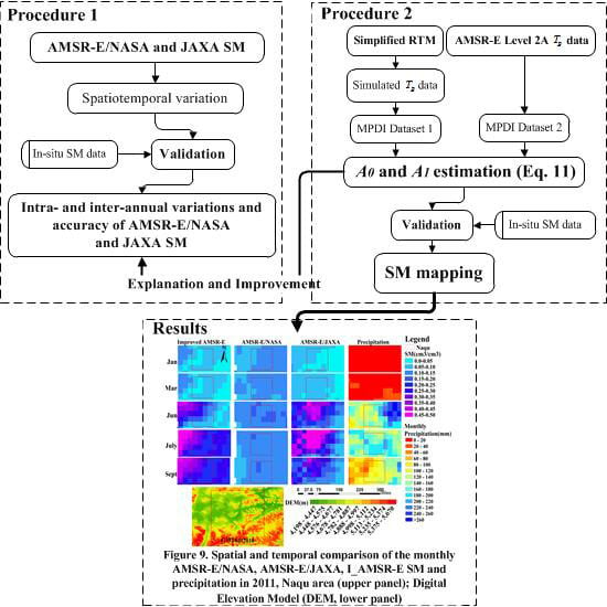
4.3. Improvement and Mapping of the AMSR-E/NASA SM Product

We applied Procedure 2 (Figure 4) to explore the possible causes of the poor accuracy of the AMSR-E/NASA SM. The analyses of the intra- and inter- annual variations of the AMSR-E/NASA and AMSR-E/JAXA SM products show that the shortcomings in the AMSR-E/NASA SM data are two-fold. On the one hand, the dynamic range of AMSR-E/NASA SM is very narrow, which does not reflect the actual intra- and inter-annual variation of precipitation (Figure 5, Figure 6 and Figure 7). On the other hand, the accuracy is poor (Table 2), with RMSE higher than 0.1 cm3 cm−3. The high RMSE values of AMSR-E/NASA are not only caused by the small dynamic range of AMSR-E/NASA soil moisture. The RMSE might have been smaller if the NASA SM would have been close to either high or low in-situ SM. The high RMSE shows that the accuracy is poor, i.e., RMSE = 0.16 cm3 cm−3, because the NASA SM is different from the in-situ SM throughout the year. It is necessary, therefore, to revisit the retrieval algorithm of the AMSR-E/NASA SM to identify the likely cause of such poor performance.
As explained in Section 3.1, we applied a simplified RTM (Equations (2)–(6)) to simulate the brightness temperature for both H and V polarized emission at 10.7 GHz. To model brightness temperature, some target properties and the observation geometry must be known. The sand and clay fractions were determined for soil samples. The soil texture is rather uniform at Naqu, and we used the mean soil textural fractions over all pixels in our numerical experiments [16]. According to the parameters of the AMSR-E sensor in Table 1, the incident angle is set as 55°. Because the Naqu area is fairly smooth with rolling hills, we estimated the surface roughness to be small, i.e., 0.03 m [16]. In summary, the area is characterized by low biomass, low vegetation water content, and similar temperature of soil and vegetation canopy. Thus, we can assume attenuation by the vegetation canopy to be low. Further, we assumed the water content of vegetation to be 1 kg/m2, the attenuation coefficient = 0.3, and single scattering albedo = 0. The in-situ measurements of SM were used in the simulation of MPDI by the simplified RTM (Equations (2)–(6)).
The monthly MPDI was calculated by applying Equation (12) to the brightness temperature data in Datasets 1 and 2 (Section 3.2 and Figure 4). As explained in Section 3.2, four different pairs of (A0, A1) were obtained (Table 3).
We used the in-situ SM data in Pixel 1, Pixel 2, Pixel 3, and Pixel 4, where we had most of our measurements, to analyze the relationship with MPDI (Figure 8). By fitting Equation (12) to both the AMSR-E/NASA and the in-situ SM data, we estimated the parameters A0 and A1 and further retrieved four sets of SM data (Figure 8). As regards the AMSR-E/NASA SM data, the A0 and A1 values were approximately the same in all pixels and equal to 1 and 0.06, respectively. As regards the in-situ data, however, we obtained A1 = 8. In other words, the value of A1 obtained by fitting Equation (12) to the AMSR-E/NASA SM product is too small and it explains the very small dynamic range. Accordingly, the model SM = 8*MPDI-0.36, i.e., (A0, A1) values obtained with the RTM MPDI + in-situ SM data (Table 1), is expected to perform better when applied to retrieve SM in our study area.
In principle, there are two different factors that can lead to large differences between the AMSR-E SM retrievals and in-situ SM measurements. First, the algorithm to retrieve SM may not be accurate, although the radiometry, i.e., the brightness temperature values, is correct. Second, the values of brightness temperature are not correct and, therefore, the MPDI values are also not correct. In this study, we assumed the brightness temperature observed by the AMSR-E sensor is correct and analyzed the AMSR-E/NASA SM retrieval algorithm.
The case (d) SM is closest to the in-situ SM data (Figure 8). In addition, by comparing case (b) with case (d), we found that the calculated SM values were close to in-situ SM measurements from January to June. From July to September, however, the SM values calculated by using case (b) SM = 8*MPDI-0.15 were much lower than the SM values calculated according to case (d) SM = 8*MPDI-0.36. The reason is that the MPDI values calculated with the AMSR-E Level 2A brightness temperature data are much lower than the MPDI values from simulated brightness temperature. The values of the AMSR-E Level 2A brightness temperature data, therefore, may not be accurate from July to September for the Tibetan Plateau. The reason may be that the TOA (top-of-atmosphere) radiance measured by AMSR-E is severely attenuated by vegetation, leading to a small difference between H and V polarization in the summer on the Tibetan Plateau.
To retrieve SM from AMSR-E Level 2A brightness temperature data from July to September, a correction for attenuation by vegetation or ex-post calibration must be applied. The good agreement of retrieved with measured SM in case (d) shows that the linear regression between the MPDI and in-situ SM data yields accurate SM retrievals and the MPDI values capture the seasonality in SM. In case (d), the brightness temperature data were simulated with the simplified RTM by applying a constant attenuation by vegetation. The same linear regression, i.e., Equation (17), applied to the AMSR-E brightness temperature observations yields accurate SM retrievals until June only. Our hypothesis is that in summer months, i.e., from July to September, vegetation biomass increases in response to snowmelt and monsoon precipitation. To estimate the correction, we opted for the simplest possible approach, i.e., by fitting a separate linear relationship to the AMSR-E MPDI values and SM measurements for all the calibration pixels and the summer months. This gave (Equation (17), July through September) a much higher and positive offset that provided the required correction. In summary, two different linear relationships must be applied to retrieve SM from the AMSR-E MPDI observations:
{ S M t = 0.15 + 8 × M P D I 10.7 t ,   ( t = 1 , 2 , 3 , 4 , 5 , 6 ) S M t = 0.05 + 8 × M P D I 10.7 t ,   ( t = 7 , 8 , 9 )  
where M P D I 10.7 t is the MPDI calculated from the AMSR-E Level 2A brightness temperature data; t is the month.
The SM retrieved from AMSR-E/NASA MPDI data by applying Equation (17) is indicated as I_AMSR-E SM. The three SM datasets, i.e., AMSR-E/NASA, AMSR-E/JAXA, and I_AMSR-E, were mapped in our Naqu study area in January, March, June, July, and September (Figure 9). There was almost no rainfall in January and March (Figure 9), while rainfall was higher in June and July. The AMSR-E/NASA SM, however, shows very limited changes from winter to summer, and SM is low from January to September. The seasonal variation of precipitation is not captured by the AMSR-E/NASA SM, while it is very evident in both the AMSR-E/JAXA SM and I_AMSR-E SM. In term of capturing the seasonal variation of soil moisture in the Naqu area, the AMSR-E/JAXA SM and I_AMSR-E SM performed better than the AMSR-E/NASA SM. In July, the I_AMSR-E SM was highest, followed by June and September. In January and March, SM was low. The I_AMSR-E SM, which fits the in-situ measurements rather well (Figure 8), remained lower than the AMSR-E/JAXA SM in June and July; this implies that our I_AMSR-E SM avoids both over- and underestimation in summer.
There are large differences in the spatial SM pattern (Figure 9) between AMSR-E/NASA, AMSR-E/JAXA and I_AMSR-E SM. AMSR-E/NASA SM is very flat and uniform in spatial distribution in the Naqu area. Compared with the AMSR-E/NASA SM spatial distribution in the Naqu area in June, the spatial dynamic range of AMSR-E/JAXA and I_AMSR-E SM is larger from 0.05 to 0.5 cm3 cm−3. Compared with the spatial pattern of precipitation in June, the precipitation is higher in the NE (Northeast) than in the NW (Northwest) portion of the Naqu area. On the other hand, both the AMRS-E/JAXA and I_AMSR-E SM are lower in the NE than in the NW portion of the Naqu area. The difference in the AMSR-E/NASA SM between the NE and NW portion is small. In comparing the spatial patterns of SM with precipitation, however, it should be taken into account that the NW portion is flatter with a large presence of water bodies, which explains the differences observed in Figure 9. We further note that our improved SM estimates (I_AMSR-E) correctly reflect the terrain, with a lower elevation catchment in the NW portion of the Naqu area.
In-situ SM measurements in Pixel 1 included 14 locations in 2011, which were divided into two sets: one subset was used to determine the linear regression (Figure 8 and Table 3), and the other subset was used for evaluation. Equation (12) was fitted to the 1st subset, i.e., 7 stations (Figure 8), while the 2nd subset was used to evaluate the I_AMSR-E SM and gave RMSE = 0.065 cm3 cm−3 (Figure 10). In conclusion, the I_AMSR-E SM compares to in-situ SM measurements better than both the AMSR-E/NASA SM (RMSE = 0.11 cm3 cm−3, Table 2) and AMSR-E/JAXA SM (RMSE = 0.10 cm3 cm−3, Table 2).

5. Discussion

The AMSR-E/NASA SM data product has an unrealistically narrow dynamic range given the hydrological conditions on the Tibetan Plateau [35,36]. By comparing the AMSR-E/NASA SM with the AMSR-E/JAXA SM, it appears that the AMSR-E/NASA SM is not sensitive to the large variations in hydrologic conditions characteristic of the Naqu site. The SM dynamic range of AMSR-E/NASA SM is very narrow and inconsistent with the in-situ measurements of SM. Our findings are confirmed by the evidence provided by [11,12]. Zeng et al., 2015 concluded that the AMSR-E/NASA SM product does not capture the soil moisture dynamics and that both AMSR-E/NASA and JAXA SM products gave relatively large RMSE values against in-situ SM measurements [11]. Chen et al., 2013 showed that the AMSR-E/NASA algorithm gave a dampened dynamic range of soil moisture while the AMSR-E/JAXA algorithm did reflect the seasonal variation of soil moisture but with too large amplitude. This implies that the AMSR-E/NASA and JAXA SM retrieval algorithms need to be improved to be applicable to the Tibetan Plateau [12]. The linear relationships between the monthly MPDI and NASA (JAXA) SM in Pixel 1 and Pixel 2 (Figure 11) show that the A1 value of NASA SM is approximately equal to 1, and the A1 value of JAXA SM is approximately equal to 8. The A1 values of 12 pixels (Figure 11e) of the relationships between the JAXA SM and MPDI were higher, i.e., over 7.67. On the other hand, for our 12 pixels, the A1 values of the relationships between the NASA SM and MPDI were very small, i.e., <1.924. This also illustrates that the AMSR-E/NASA SM does not reflect the dynamics of soil moisture but AMSR-E/JAXA can. Although the AMSR-E/NASA SM is considered a reference data set by the National Snow & Ice Data Center (NSIDC), the narrow dynamic range of SM seriously limits its application to drought and environmental change monitoring and other applications [13].
Two results given above point to the same possible cause. We have shown that a simple linear relationship (Equation (17)) with a slope equal to 8 gives accurate SM retrievals when the brightness temperature is calculated from in-situ SM measurements (Case d in Figure 8 and Table 3). When applying the same linear relationship to the AMSR-E brightness temperature data, the retrieved SM is severely underestimated in summer, i.e., under wet conditions, and the offset parameter in our linear relationship (Equation (17)) had to be recalculated to improve accuracy of the retrieved SM. Both slope and offset in Equation (17) are related to the g* parameter (Equation (9)), which should be evaluated for each month and location. We note that a time-dependent g* would correct for seasonal variations in attenuation by the vegetation canopy of soil emittance. Our results (Table 3) on the slope parameter A1 of the linear relationship (Equation (17)) show that the sensitivity of the NASA SM retrieval algorithm to actual soil moisture changes may not be adequate. These results indicated that the value of A1 in Equation (17) should be much higher, i.e., 8 instead of 1. This difference explains the unrealistically narrow dynamic range of the AMSR-E/NASA SM for the Tibetan Plateau. Zeng et al. (2015) noted that the parameters of the AMSR-/NASA SM retrieval algorithm were determined by calibration in specific regions, with the risk of the algorithm being not suitable to retrieve SM in other regions [11,12]. We are aware that the AMSR-E/NASA SM algorithm performed relatively well in Mongolia and the United States [5], although it did not provide accurate SM retrievals for the Tibetan Plateau [11,37]. It has been suggested by other authors that these parameters (Equations (7)–(9)) should be recalibrated in other areas besides the Tibetan Plateau to improve the accuracy of SM retrievals in these regions [11,13].
We have evaluated the AMSR-E/NASA SM just in one study area, i.e., Naqu on the Tibetan Plateau, but we concluded that the reason leading to the unrealistically narrow dynamic range of AMSR-E/NASA SM was the very low value, i.e., 1 instead of 8, of the parameter A 1 = a 1 · exp ( a 2 · g ) which is related as shown to the parameters in the AMSR-E/NASA SM algorithm. We believe there might be other areas, besides Naqu, potentially affected by the same problem; thus, we repeated our evaluation in a second experiment.
We chose an area in Poland, where the dynamic range of the AMSR-E/NASA SM is also small, notwithstanding a large seasonal variation in precipitation, and estimated our linear regression Equation (12) using in-situ SM measurements. More specifically, we evaluated the cases (a) and (b) in Table 1, which gave A1 = 4 when using the AMSR-E/NASA MPDI and NASA SM against A1 = 32 when using the AMSR-E/NASA MPDI and in-situ SM. This recalibration improved accuracy very significantly (Figure 12), and the improved SM retrievals perfectly captured the seasonality in precipitation (Figure 12). We note that also in this case, the AMSR-E/NASA SM remained nearly constant throughout the year and did not respond at all to the large variation in precipitation. As with the Naqu case, the large improvement in accuracy could be achieved by applying a higher A1 value in Equation (12). It might be useful to recall here that the parameter values in the relation between MPDI and parameter g* built-in the AMSR-E NASA algorithm come from the calibration established with observations in portions of Chad, Sudan and the Central African Republic. This might explain why A1=8 or larger A1 are obtained when using in-situ SM measurements instead of the AMSR-E/NASA SM retrievals. We may speculate further that this calibration did not capture adequately the sensitivity of MPDI to actual soil moisture conditions.
In conclusion, we believe there are likely other regions where the dynamic range of the AMSR-E/NASA SM is too narrow, given actual hydrologic conditions. In these regions, the coefficients in the AMSR-E/NASA SM algorithm are not suitable to retrieve SM and should be re-calibrated, leading to significantly higher accuracy.

6. Conclusions

This work shows an analysis, comparison and improvement of AMSR-E soil moisture data products in the Naqu area, Tibetan Plateau, in 2011. Our spatiotemporal analysis of AMSR-E/NASA and AMSR-E/JAXA SM products documented the differences in the two SM products. The dynamic range of the AMSR-E/NASA SM product is very narrow, which does not reflect the intra- and inter-annual variations in hydrologic conditions. The AMSR-E/NASA SM value was almost a constant, i.e., 0.12 cm3 cm−3 (Figure 5) throughout the year, while the AMSR-E/JAXA SM performed better than that. Furthermore, by fitting the MPDI values to AMSR-E/NASA and in-situ SM data, the values of the slope A1 (Equation (12)) were approximately equal to 1 and 8, respectively (Table 3). When A1 = 8, the SM estimated by the improved model (Equation (13)) was much closer to the in-situ SM measurements than the AMSR-E/NASA SM data, with RMSE = 0.065 cm3 cm−3 (Figure 10). The AMSR-E/NASA SM is generated with A1 = 1, i.e., too small, given the actual intra-annual soil moisture dynamic range in Naqu, Tibetan Plateau. In addition, from July to September in 2011, the calculated MPDI from AMSR-E brightness temperature data is small, leading to low SM calculated by using case b): SM = MPDI*8-0.15 in Table 2. The reason may be the influence of vegetation on the radiance measured by AMSR-E in this period, which leads to a small difference between H and V polarization. Therefore, there are two reasons of the narrow intra- and inter-annual variation of AMSR-E/NASA SM: the value of the A1 parameter is too small, and the calculated MPDI value from AMSR-E Level 2A brightness temperature data is small in summer.
By applying the method described in this study, we obtained A1 = 8 using in-situ SM measurements in the Naqu area, Tibetan Plateau and A1 = 32 using in-situ SM measurements in Poland. Therefore, in different regions, the A1 value is different and needs to be calibrated. In Figure 11, in Pixel 1 and Pixel 2, the A1 value obtained from the relationships built between the JAXA SM and MPDI is similar to the values obtained from the relationship between the in-situ SM measurements and MPDI i.e., A1 = 8. Therefore, in Pixel 1 and Pixel 2 of Naqu study area, JAXA SM instead of in-situ SM measurements might be used to re-calibrate the parameters in the NASA algorithm, since similar A1 values are obtained with in-situ SM measurements and with the JAXA SM products (see Figure 11). This suggests an option to re-calibrate the parameters in the NASA algorithm (Equations (7)–(9)). Particularly, this idea might be useful to calibrate the A1 value in other regions when no in-situ SM measurements are available. A broader perspective along the same line of thinking is to make use of the in-situ SM measurements collected at the ISMN sites and produce a global map of A1 towards improved accuracy of the NASA SM data.

Author Contributions

This study was designed and completed through collaboration among all the authors, Q.X., M.M. and L.J., Q.X. prepared and processed the AMSR-E/NASA, AMSR-E/JAXA and in-situ measurements datasets, performed the main analysis and wrote this manuscript. M.M. contributed important ideas, revising and editing multiple versions of this manuscript. L.J. provided key comments and revised this manuscript including figures and formulas.

Funding

This work was jointly supported by the Strategic Priority Research Program of the Chinese Academy of Sciences (Grant No. XDA19030203), the National Natural Science Foundation of China project (Grant No. 41661144022), the NRSCC—ESA Dragon—4 project (Grant N0.32439), and the MOST High Level Foreign Expert program (Grant No. G20190161018). And the APC was funded by the Strategic Priority Research Program of the Chinese Academy of Sciences (Grant No. XDA19030203).

Acknowledgments

Thanks are extended to Kun Yang et al. for providing in-situ soil moisture data for the Naqu area. The authors would like to thank the NSIDC for the AMSR-E/NASA soil moisture product and the Globe Portal System (G-Portal) for the AMSR-E/JAXA soil moisture product. We were very thankful the valuable comments from the reviewers that helped us to improve our manuscript.

Conflicts of Interest

All authors declare no conflict of interest.

References

  1. Karthikeyan, L.; Pan, M.; Wanders, N.; Kumar, D.N.; Wood, E.F. Four decades of microwave satellite soil moisture observations: Part 1. A review of retrieval algorithms. Adv. Water Resour. 2017, 109, 106–120. [Google Scholar] [CrossRef]
  2. Karthikeyan, L.; Pan, M.; Wanders, N.; Kumar, D.N.; Wood, E.F. Four decades of microwave satellite soil moisture observations: Part 2. Product validation and inter-satellite comparisons. Adv. Water Resour. 2017, 109, 236–252. [Google Scholar] [CrossRef]
  3. Njoku, E.G.; Jackson, T.J.; Lakshmi, V.; Chan, T.K.; Nghiem, S.V. Soil moisture retrieval from AMSR-E. IEEE Trans. Geosci. Remote Sens. 2003, 41, 215–229. [Google Scholar] [CrossRef]
  4. Njoku, E.; Koike, T.; Jackson, T.; Paloscia, S. Retrieval of Soil Moisture from AMSR Data; Vsp Publishing: Utrecht, The Netherlands, 1999; pp. 525–533. [Google Scholar]
  5. Jackson, T.J.; Cosh, M.H.; Bindlish, R.; Starks, P.J.; Bosch, D.D.; Seyfried, M.; Goodrich, D.C.; Moran, M.S.; Du, J.Y. Validation of advanced microwave scanning radiometer soil moisture products. IEEE Trans. Geosci. Remote Sens. 2010, 48, 4256–4272. [Google Scholar] [CrossRef]
  6. Koike, T.; Njoku, E.; Jackson, T.J.; Paloscia, S. Soil moisture algorithm development and validation for the ADEOS-II/AMSR. In Proceedings of the IGARSS 2000, IEEE 2000 International Geoscience and Remote Sensing Symposium, Taking the Pulse of the Planet: The Role of Remote Sensing in Managing the Environment. Proceedings (Cat. No.00CH37120), Honolulu, HI, USA, 24–28 July 2000. [Google Scholar]
  7. Paloscia, S.; Macelloni, G.; Santi, E.; Koike, T. A multifrequency algorithm for the retrieval of soil moisture on a large scale using microwave data from SMMR and SSM/I satellites. IEEE Trans. Geosci. Remote Sens. 2001, 39, 1655–1661. [Google Scholar] [CrossRef]
  8. Cho, E.; Su, C.; Ryu, D.; Kim, H.; Choi, M. Does AMSR2 produce better soil moisture retrievals than AMSR-E over Australia? Remote Sens. Environ. 2017, 188, 95–105. [Google Scholar] [CrossRef]
  9. Feng, X.; Li, J.; Cheng, W.; Fu, B.; Wang, Y.; Lü, Y.; Shao, M. Evaluation of AMSR-E retrieval by detecting soil moisture decrease following massive dryland re-vegetation in the Loess Plateau, China. Remote Sens. Environ. 2017, 196, 253–264. [Google Scholar] [CrossRef]
  10. Lu, H.; Koike, T.; Fujii, H.; Ohta, T.; Tamagawa, K. Development of a Physically-based Soil Moisture Retrieval Algorithm for Spaceborne Passive Microwave Radiometers and its Application to AMSR-E. J. Remote Sens. Soc. Jpn. 2009, 29, 253–262. [Google Scholar]
  11. Zeng, J.; Zhen, L.; Quan, C.; Bi, H.; Qiu, J.; Zou, P. Evaluation of remotely sensed and reanalysis soil moisture products over the Tibetan Plateau using in-situ observations. Remote Sens. Environ. 2015, 163, 91–110. [Google Scholar] [CrossRef]
  12. Chen, Y.; Yang, K.; Qin, J.; Zhao, L.; Tang, W.; Han, M. Evaluation of AMSR-E retrievals and GLDAS simulations against observations of a soil moisture network on the central Tibetan Plateau. J. Geophys. Res. Atmos. 2013, 118, 4466–4475. [Google Scholar] [CrossRef]
  13. Zeng, J.; Zhen, L.I.; Chen, Q.; Haiyun, B.I. A simplified physically-based algorithm for surface soil moisture retrieval using AMSR-E data. Front. Earth Sci. 2014, 8, 427–438. [Google Scholar] [CrossRef]
  14. Lacava, T.; Brocca, L.; Faruolo, M.; Matgen, P.; Moramarco, T.; Pergola, N.; Tramutoli, V. A multi-sensor (SMOS, AMSR-E and ASCAT) satellite-based soil moisture products inter-comparison. In Proceedings of the 2012 IEEE International Geoscience and Remote Sensing Symposium, Munich, Germany, 22–27 July 2012. [Google Scholar]
  15. Kang, C.S.; Kanniah, K.D. Validation of AMSR-E soil moisture product and the future perspective of soil moisture estimation using SMOS data over tropical region. In Proceedings of the 2013 IEEE International Geoscience and Remote Sensing Symposium—IGARSS, Melbourne, Australia, 21–26 July 2013. [Google Scholar]
  16. Yang, K.; Qin, J.; Zhao, L.; Chen, Y.; Han, M. A Multi-Scale Soil Moisture and Freeze-Thaw Monitoring Network on the Third Pole. Bull. Am. Meteorol. Soc. 2013, 94, 1907–1916. [Google Scholar] [CrossRef]
  17. Njoku, E.G.; Chan, S.K. Vegetation and surface roughness effects on AMSR-E land observations. Remote Sens. Environ. 2006, 100, 190–199. [Google Scholar] [CrossRef]
  18. Chen, Y.; Yang, K.; Qin, J.; Cui, Q.; Lu, H.; La, Z.; Han, M.; Tang, W. Evaluation of SMAP, SMOS, and AMSR2 soil moisture retrievals against observations from two networks on the Tibetan Plateau. J. Geophys. Res. Atmos. 2017, 122, 5780–5792. [Google Scholar] [CrossRef]
  19. Lu, H.; Koike, T.; Yang, K.; Hu, Z.; Xu, X.; Rasmy, M.; Kuria, D.; Tamagawa, K. Improving land surface soil moisture and energy flux simulations over the Tibetan plateau by the assimilation of the microwave remote sensing data and the GCM output into a land surface model. Int. J. Appl. Earth Obs. Geoinf. 2012, 17, 43–54. [Google Scholar] [CrossRef]
  20. Liu, Q.; Shi, J.; Du, J.; Zhang, S. Soil moisture retrieval by remote sensing and multi-year trend analysis of the soil moisture in Tibetan Plateau. In Proceedings of the 2012 IEEE International Geoscience and Remote Sensing Symposium, Munich, Germany, 22–27 July 2012. [Google Scholar]
  21. Zhao, T.J.; Zhang, L.X.; Shi, J.C.; Jiang, L.M. A physically based statistical methodology for surface soil moisture retrieval in the Tibet Plateau using microwave vegetation indices. J. Geophys. Res. 2011, 116, 5229. [Google Scholar] [CrossRef]
  22. Zhao, L.; Yang, K.; Qin, J.; Chen, Y.; Tang, W.; Lu, H.; Yang, Z. The scale-dependence of SMOS soil moisture accuracy and its improvement through land data assimilation in the central Tibetan Plateau. Remote Sens. Environ. 2014, 152, 345–355. [Google Scholar] [CrossRef]
  23. Yang, K.; Zhu, L.; Chen, Y.; Zhao, L.; Qin, J.; Lu, H.; Tang, W.; Han, M.; Ding, B.; Fang, N. Land surface model calibration through microwave data assimilation for improving soil moisture simulations. J. Hydrol. 2016, 533, 266–276. [Google Scholar] [CrossRef]
  24. Wang, L.; Li, Z.; Ren, X. The effects of vegetation in soil moisture retrieval using microwave radiometer data. In Proceedings of the IGARSS 2004. 2004 IEEE International Geoscience and Remote Sensing Symposium, Anchorage, AK, USA, 20–24 September 2004. [Google Scholar]
  25. Parkinson, C.L. Aqua: an Earth-Observing Satellite mission to examine water and other climate variables. IEEE Trans. Geosci. Remote Sens. 2003, 41, 173–183. [Google Scholar] [CrossRef]
  26. Du, J.; Kimball, J.S.; Jones, L.A.; Kim, Y.; Glassy, J.; Watts, J.D. A global satellite environmental data record derived from AMSR-Eand AMSR2 microwave earth observations. Earth Syst. Sci. Data Discuss. 2017, 9, 791–808. [Google Scholar] [CrossRef]
  27. Kolassa, J.; Gentine, P.; Prigent, C.; Aires, F.; Alemohammad, S.H. Soil moisture retrieval from AMSR-E and ASCAT microwave observation synergy. Part 2: Product evaluation. Remote Sens. Environ. 2017, 195, 202–217. [Google Scholar] [CrossRef]
  28. Njoku, E.; Chan, T.; Crosson, W.; Limaye, A. Evaluation of the AMSR-E data calibration over land. Holography 2004, 11, 1–28. [Google Scholar]
  29. Njoku, E.G.; Ashcroft, P.; Chan, T.K.; Li, L. Global survey and statistics of radio-frequency interference in AMSR-E land observations. IEEE Trans. Geosci. Remote Sens. 2005, 43, 938–947. [Google Scholar] [CrossRef]
  30. Mo, T.; Choudhury, B.J.; Schmugge, T.J.; Wang, J.R.; Jackson, T.J. A model for microwave emission from vegetation-covered fields. J. Geophys. Res. Ocean. 1982, 87, 11229–11237. [Google Scholar] [CrossRef]
  31. Lu, H.; Koike, T.; Fujii, H.; Ohta, T.; Tamagawa, K. Monitoring soil moisture change in North Africa with using satellite remote sensing and land data assimilaiton system. In Proceedings of the 2009 IEEE International Geoscience and Remote Sensing Symposium, Cape Town, South Africa, 12–17 July 2009. [Google Scholar]
  32. Li, L.; Njoku, E.G.; Im, E.; Chang, P.S.; Germain, K.S. A preliminary survey of radio-frequency interference over the U.S. in Aqua AMSR-E data. IEEE Trans. Geosci. Remote Sens. 2004, 42, 380–390. [Google Scholar] [CrossRef]
  33. Mladenova, I.; Lakshmi, V.; Jackson, T.J.; Walker, J.P.; Merlin, O.; de Jeu, R.A.M. Validation of AMSR-E soil moisture using L-band airborne radiometer data from National Airborne Field Experiment 2006. Remote Sens. Environ. 2011, 115, 2096–2103. [Google Scholar] [CrossRef]
  34. Xie, Q.; Meng, Q.; Zhang, L.; Wang, C.; Sun, Y.; Sun, Z. A Soil Moisture Retrieval Method Based on Typical Polarization Decomposition Techniques for a Maize Field from Full-Polarization Radarsat-2 Data. Remote Sens.-Basel. 2017, 9, 168. [Google Scholar] [CrossRef] [Green Version]
  35. Qi, Y.; Lu, L.; Jiang, L.; Tao, J.; Du, J.; Shi, J. Tibetan Plateau Soil Moisture Products Intercomparison and the Field Observations; American Geophysical Union Fall Meeting: Washington, DC, USA, 2002. [Google Scholar]
  36. Xi, J.; Wen, J.; Tian, H.; Zhang, T. Applicability evaluation of AMSR-E remote sensing soil moisture products in Qinghai-Tibet plateau. Trans. Chin. Soc. Agric. Eng. 2014, 30, 194–202. [Google Scholar]
  37. Zeng, J.; Zhen, L.; Quan, C.; Bi, H.; Ping, Z. A physically-based algorithm for surface soil moisture retrieval in the Tibet Plateau using passive microwave remote sensing. In Proceedings of the 2013 IEEE International Geoscience and Remote Sensing Symposium—IGARSS, Melbourne, Australia, 21–26 July 2013. [Google Scholar]
Figure 1. Overview of the algorithms used to retrieve the AMSR-E/NASA and AMSR-E/JAXA SM.
Remotesensing 11 02748 g001
Figure 2. Location and land cover types of the study area and in-situ sites in Naqu on the Tibetan Plateau. A: histogram of land cover types at the locations of in-situ SM measurements in Pixel 1; B: histogram of land cover types of Pixel 1 with 25 km × 25 km; land cover based on the GLOBCOVER 2009 map at 300 m × 300 m spatial resolution.
Remotesensing 11 02748 g002
Figure 3. Relationships between the monthly AMSR-E/NASA and JAXA SM values and monthly MPDI in the Naqu area of the Tibetan Plateau in 2011: (a) NASA SM, all pixels; (b) JAXA SM, all pixels.
Remotesensing 11 02748 g003
Figure 4. Flow chart of AMSR-E/NASA, JAXA SM product analysis and improving the AMSR-E SM product.
Remotesensing 11 02748 g004
Figure 5. The monthly mean SM and standard deviation of AMSR-E/NASA and AMSR-E/JAXA retrievals for the same 2000 pixels for the Tibetan Plateau from 2002 to 2011: (a) SM retrieved with data collected during ascending orbits and (b) descending orbits; (c) SM standard deviation for ascending orbits, and (d) descending orbits.
Remotesensing 11 02748 g005aRemotesensing 11 02748 g005b
Figure 6. Comparison of AMSR-E/NASA or JAXA SM products with in-situ SM measurements data in 2011: (a) AMSR-E/NASA during ascending orbits and (b) descending orbits; (c) AMSR-E/JAXA during ascending orbits, and (d) descending orbits.
Remotesensing 11 02748 g006aRemotesensing 11 02748 g006b
Figure 7. Intra-annual variation and relative anomaly of AMSR-E/NASA, JAXA SM data and in-situ SM measurements in Pixel 1, 2011: (A) AMSR-E/NASA during ascending orbits and (B) descending orbits; (C) AMSR-E/JAXA during ascending orbits, and (D) descending orbits.
Remotesensing 11 02748 g007aRemotesensing 11 02748 g007b
Figure 8. Monthly in-situ SM measurements and AMSR-E/NASA SM for the four cases in Table 1; Pixel 1 through Pixel 4 (A: Pixel 1; B: Pixel 2; C: Pixel 3; D: Pixel 4) in the Naqu area in 2011.
Remotesensing 11 02748 g008
Figure 9. Spatial and temporal comparison of the monthly AMSR-E/NASA, AMSR-E/JAXA, I_AMSR-E SM and precipitation in January, March, June, July and September in 2011, the Naqu area (upper panel); Digital Elevation Model (DEM, lower panel).
Remotesensing 11 02748 g009
Figure 10. Monthly I_AMSR-E, AMSR-E/NASA and JAXA SM retrievals and in-situ SM measurements in Pixel 1 in the Naqu area of the Tibetan Plateau in 2011.
Remotesensing 11 02748 g010
Figure 11. Relationships between the monthly AMSR-E/NASA and JAXA SM values and monthly MPDI in pixels 1 through 12, Naqu area in 2011; (a) NASA SM Pixel 1; (b) NASA SM Pixel 2; (c) JAXA SM Pixel 1; (d) NASA SM Pixel 2; (e) the A1 coefficient values.
Remotesensing 11 02748 g011
Figure 12. Poland study area SM in 2011, cases a) and b) in Table 1, AMSR-E/NASA SM product and in-situ SM measurements, and precipitation.
Remotesensing 11 02748 g012
Table 1. Summary of long time series of soil moisture data retrieved from passive microwave radiometer observations (SR: spatial resolution; IA: incidence angle).
Microwave SensorsSM ProductsPeriodIA (°)Frequency (GHz)SRUnitSpatial CoverageAlgorithms
SMMR/1978–198750.26.6, 10.7//Global/
SSM/I/1987–200753.119.35//Global/
TRMM/TMIL31997–201552.810.725 kmcm3/cm3180W-180E, 50S-50NLPRM (Owe et al., 2008)
AMSR-EJAXA2002–2011556.9, 10.7, 36.525 kmcm3/cm3GlobalLUT (Du et al., 2009)
NASA2002–2011556.9, 10.7, 36.525 kmcm3/cm3GlobalNjoku (Njoku et al., 2003 and 2006)
IRSA2002–2011556.9,10.725 kmcm3/cm3GlobalQP (Shi et al.2006)
VUA2002–2011556.9, 10.725 kmcm3/cm3GlobalLPRM (Owe et al., 2008)
WindSatL32003–201250.16.8, 10.725 kmcm3/cm3180W-180E, 64S-83NLPRM (Owe et al., 2008)
AMSR2L32012–present556.93, 7.3, 10.6525 kmcm3/cm3GlobalLPRM/LUT (Owe et al., 2008, Du et al., 2009)
MWRI/FY3L22011–present5310.6525 kmcm3/cm3GlobalQP (Shi et al.2006)
MIRAS/SMOSCATDS-L32010–present2.5–62.51.4125 kmcm3/cm3GlobalL-MEB (Kerr et al.,2012)
SMAPL32015–present401.41, 1.26 (SAR)3/9/36 kmcm3/cm3180W-180E, 85S-85N SCA (O’Neill et al.,2016)
Table 2. Calculated MAE, RMSE, and R of SM data in the Naqu area against in-situ SM measurements in 2011; st. dev are the standard deviation of each SM data product for each pixel, respectively.
AMSR-E/NASAAMSR-E/JAXA
MAERMSERStd. DevMAERMSERStd. Dev
Pixel 10.090.110.720.0170.060.100.910.128
Pixel 20.080.100.720.0160.070.090.880.143
Pixel 30.090.120.660.0140.070.110.800.175
Pixel 40.120.160.640.0190.090.100.880.123
Pixel 50.200.250.480.0130.120.150.820.175
Pixel 60.060.070.670.0170.030.040.870.101
Pixel 70.120.150.610.0180.070.100.830.105
Pixel 80.150.180.540.0140.090.110.860.118
Pixel 90.150.180.600.0120.120.150.880.085
Pixel 100.130.150.410.0150.080.100.860.078
Pixel 110.200.220.620.0140.100.120.840.167
Pixel 120.190.200.720.0180.070.090.790.145
Average0.130.160.620.0150.080.110.850.129
Table 3. Values of A0 and A1 parameters (see text for details on the estimation procedure).
CasesA1A0
(a) AMSR-E/NASA MPDI + NASA SM10.09
(b) AMSR-E/NASA MPDI + in-situ SM8−0.15
(c) RTM MPDI + NASA SM10.06
(d) RTM MPDI + in-situ SM8−0.36

