A Statistical Forest Reflectance Model

Abstract

The variability of forest reflectance among hemiboreal forests can be described with a few basis functions. Five basis functions describe almost 98% of variability of directional reflectance spectra in the optical spectral domain (400–1700 nm) in forest stands at the top of a canopy in nadir. A statistical forest reflectance model (SFRM) was developed, the input parameters of which are the forest parameters measured in the course of regular forest inventory. Nadir spectral reflectance of a forest stand is expressed in the SFRM as a linear combination of basis functions, the weights of which are linear combinations of the 15 stand parameters in the forest inventory database. Multiple correlations of the weights on the forest inventory parameters are determined separately for pine, spruce, and broadleaf forests. The basis functions are found from low altitude airborne measurements over managed forests in southeastern Estonia, where a forest management database is available. The model was validated against more than 3000 spectral signatures of forest stands from Sentinel-2 Multispectral Imager (MSI) measurements over a test site in southeastern Estonia. In most cases, the model predicts the forest reflectance spectrum at nadir with a relative error about 20–40%. The errors of reflectance values are less than 0.02 in most cases. The sole exception is the reflectance of broadleaf stands, which in near infrared bands of Sentinel-2 MSI is overestimated by 0.02–0.05.

1. Introduction

Interaction of solar radiation and vegetation controls the energy budget of vegetated ground, photosynthesis, and transpiration from the vegetation cover. Optical remote sensing of land cover is based on the measurements of scattered and reflected solar radiation. Interaction of solar radiation and vegetation is described with radiative transfer models. The development of physical radiative transfer models for vegetation canopies has become an effort spanning several decades [1,2,3,4]. Physical forest reflectance models describe the interaction of radiation with an extremely heterogeneous and variable forest canopy. Such models have a long list of input parameters, as a rule [3,4,5]. In model simulations, it is almost impossible to measure values of all necessary input parameters, whether in field campaigns or in the laboratory. The collection of input parameter values is challenging even where forest inventory data are available. Forest management inventory databases include stand parameters which foresters have found necessary for describing a forest stand. The set of parameters has taken shape over decades of practical inventory for forest management [6,7]. A number of forest parameters, such as species composition, age, breast-height diameter, tree height, basal area, stem volume, and site type, are provided in such databases. On the other hand, several optical and structure parameters which are needed in forest radiative transfer models are missing or difficult to estimate from forest inventory data [8]. Therefore, literature data or some expert guess must be used for such model input parameters. The situation becomes still more complex when trying to solve the inverse problem, of estimating some forest parameters from reflectance-spectra measurements. It appears that reflectance spectra of various forest stands are rather similar, and only a few forest parameters can be estimated in an inversion.

The dimensionality of remote sensing measurements has increased over time. While the most common optical vegetation characteristic, the normalized difference vegetation index (NDVI), is constructed from two spectral bands, and while the main optical satellite sensor, the Landsat Thematic Mapper, in land cover remote sensing over the past couple of decades had six optical spectral bands, the spectral resolution and the number of spectral bands of remote sensing sensors have in recent years, increased substantially. The current reality involves spectral resolutions under 10 nm, with the count of spectral bands now numbering from the tens up to a few hundred [9,10,11]. The result of that is the enormous size increase of remote sensing databases, and of required storage.

Computational methods of spectral analysis and inverse-problem solution encounter difficulties if the dimensionality of measurements becomes large. The inversion of very high dimensionality matrices is computationally intensive and subject to rounding errors. The existence of noise and spectral redundancy in the data can cause matrix inversion to fail. Observational data can be condensed through fitting to a model that depends on adjustable parameters. The model can be simply a convenient class of functions, with the fit supplying the appropriate coefficients. Such functions are called the basis functions [12]. The basic approach is the design of a merit function, as a measure of the agreement between data and model. Both the basis functions and their coefficients then have to be found through minimization of this merit function. This problem is solved through an application of general least squares [12]. A similar procedure was first used by Price [13] for the analysis of reflectance spectra of soil samples. The variability of the reflectance spectra of 564 soil samples in the wavelength range of 0.55–2.32 $\mathsf{\mu }$m and the dimensionality of $n=178$ was represented by the sum of four orthogonal basis functions. The spectral discrimination of these soils relied on at most four independent variables, and the space of measurements for the 564 soils was spanned by four fitting functions—tabulated basis vectors of dimensionality $n=178$.

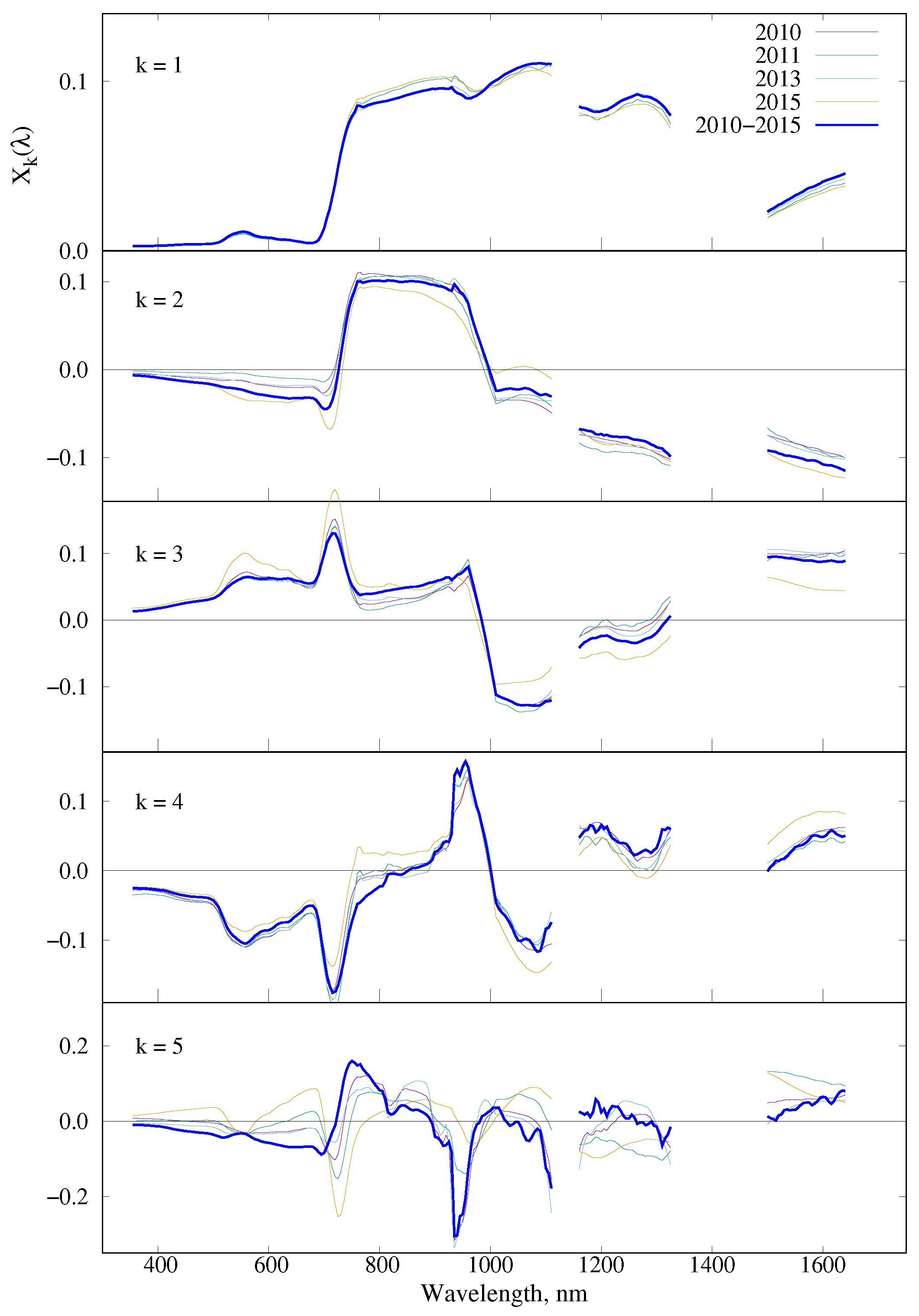
A similar approach can be used for forest reflectance. The forest reflectance spectra can be estimated by finding a set of basis functions which explains the variability of forest reflectance spectra, and determining the weights for these basis functions. We seek these weights as the function of forest inventory parameters which are the most comprehensive description of a managed forest stand, and are usually available for most of the stands. The weights of basis functions are expressed as the multiple regression of forest inventory parameters. In this way, a statistical model of forest reflectance (SFRM) is obtained, the input parameters of which are the stand parameters provided by the regular forest inventory. Basis functions are found by analyzing the variability of measured forest reflectance spectra over hemiboreal forests in southeastern Estonia for which a forest management inventory database is available. The results from a comparison of the simulated and the measured spectra are reported.

2. Material and Methods

Airborne measurements of directional reflectance in the spectral range 355–1640 nm were carried out over hemiboreal forests at the Järvselja test site in southeastern Estonia in 2010–2015. The coordinates of the test site are 58.3°N, 27.3°E. The landscape at the test site is a plain, with ground height 30–40 m asl. The site harbors mixed forests from the hemiboreal zone, with a moderately cool and moist climate. These forests are managed. Nevertheless, they can be characterized as remote and rural with low anthropogenic disturbances. Stands are pure or mixed, and composed mainly of silver birch (Betula pendula), Scots pine (Pinus sylvestris), Norway spruce (Picea abies), common alder (Alnus glutinosa), aspen (Populus tremula), gray alder (Alnus incana), and small-leaved lime (Tilia cordata). A forest management inventory database which follows the concepts by Burkhart and Tomé [6], Ferretti and Fisher [7] is available for the Järvselja Training and Experimental Forest district. The stand-wise inventory is in compliance with Estonian forest inventory regulations [14]. Forest stands are delineated using aerial photos, data from a previous inventory, and field visits, so as to yield a 1:10,000 map. A forest stand is a patch of forest homogeneous in species composition, age, tree height, tree density, and site type. The main forest inventory variables measured in the field for forest stand elements (a combination of tree species, dominance, and age) are height, stand basal area, and diameter of stems at breast height. Tree species composition in each social layer is calculated according to the wood volume of trees. Stand relative density is the ratio of stand basal area to the standard value according to forest height. The database is updated regularly. The primary forest parameters in the database are listed in

Table 1. The primary forest parameters.

Parameter	Range
Stand age	6–246 years
Percent of main species	30–100%
Stand height	1–36 m
Relative density of the upper layer	0–145%
Relative density of the lower layer	0–62%
Basal area of the upper layer	0–45 m${}^2$/ha
Basal area of the lower layer	0–17 m${}^2$/ha
Stem volume of the upper layer	0–623 m${}^3$/ha
Stem volume of the lower layer	0–162 m${}^3$/ha
Percent of birch	1–100%
Percent of aspen	1–100%
Percent of common alder	1–100%
Percent of gray alder	1–100%
Percent of pine	1–100%
Percent of spruce	1–100%

.

Although some additional tree species are listed in the database, their share in the forests under study is negligible.

Under the forest inventory rules, the minimum area of a stand is 0.1 ha. Growth conditions at the study site range from poor, where the site index H${}_{100}$ is less than 10 m, to very good, where H${}_{100}$ can be over 35 m. The site index H${}_{100}$ is the stand height at the stand age of 100 years. About 75% of the site area is comprised of forests, natural grasslands, and pastures. A more detailed description of the test site is provided by Kuusk et al. [15].

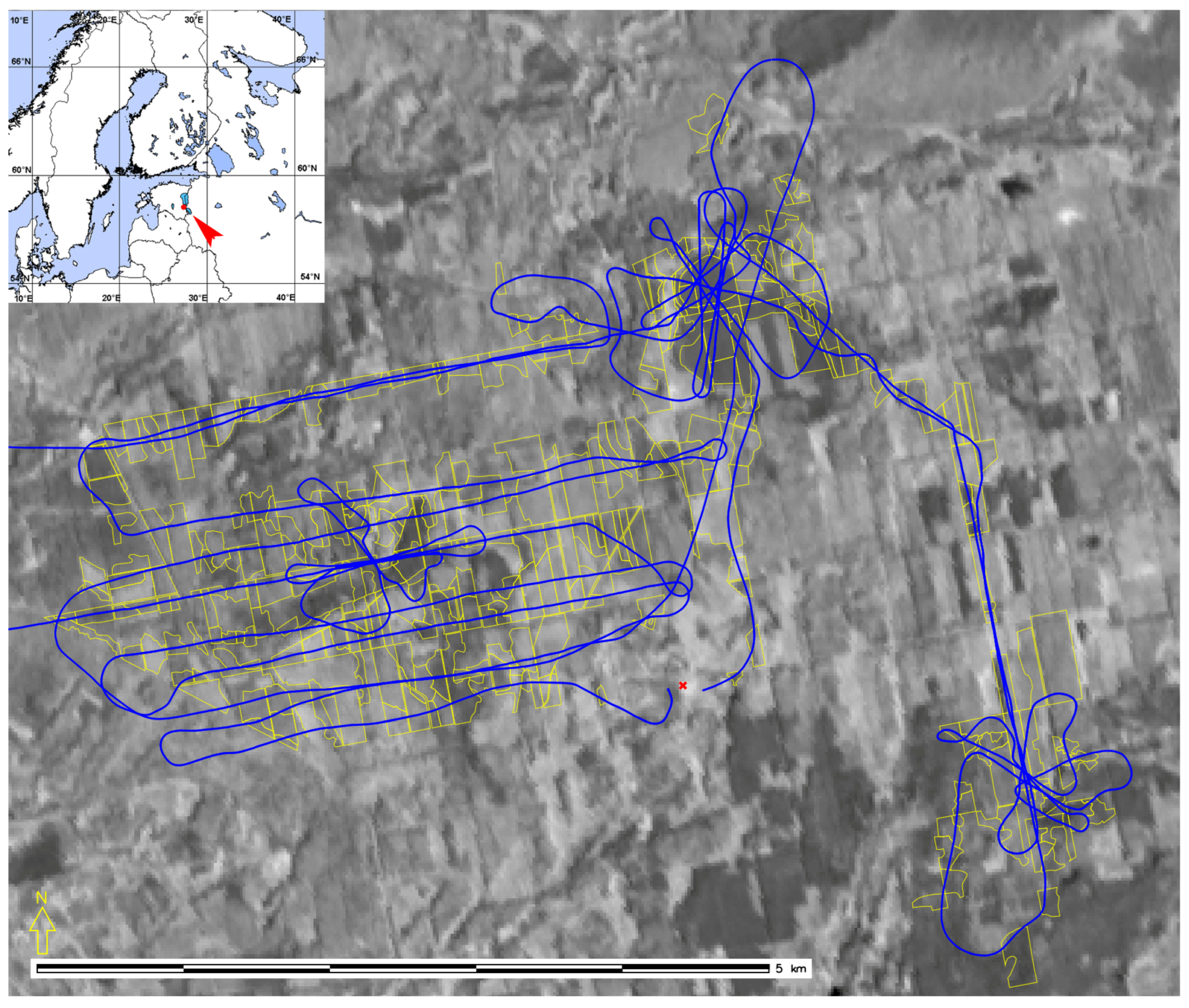
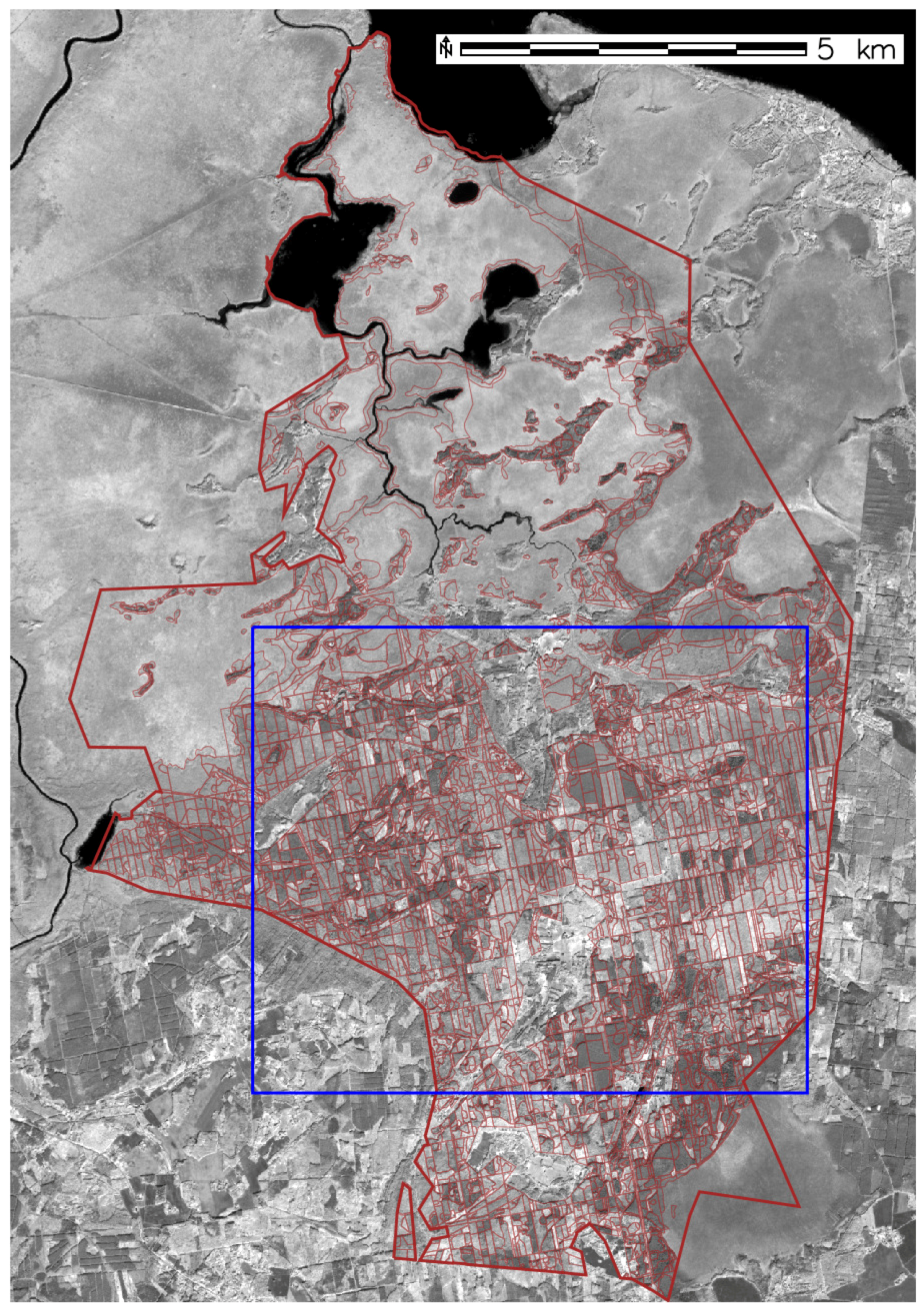
Helicopter measurements of reflectance spectra in the spectral domain 355–1640 nm over the study area were carried out using the spectrometers UAVSpec3 and UAVSpec4SWIR on 5 July 2010, 27 July 2011, 29 July 2013, and 21 July 2015. The sun zenith angle (SZA) was close to 40° during all measurements. Figure 1 shows the flight route in 2010. The same area was covered by airborne measurements in other years. Yellow polygons in the figure mark the stands involved in this study for model construction. The number of measured stands varied from year to year: 335 in 2010, 298 in 2011, 360 in 2013, and only 240 in 2015 because emerging clouds interrupted the measurements. Altogether, 578 stands were measured. As several stands were measured in more than one year, the total number of spectral signatures involved in the study was 1233.

The spectrometers UAVSpec3 and UAVSpec4SWIR are fully autonomous, lightweight spectrometers based on the 256-band miniature visible-near infrared (VisNIR) and shortwave infrared (SWIR) spectrometer modules by Carl Zeiss Jena GmbH [11]. The spectral resolution of both spectrometers is 10 nm. Recorded spectra were resampled to the spectral step of 5 nm. Reflectance values in the absorption band of water vapor were removed, because of their adverse effect on the signal-to-noise ratio. Each recorded spectrum consequently covers the ranges 355–1110 nm, 1160–1325 nm, and 1500–1640 nm, yielding a total of 217 spectral values.

The spectrometers were mounted on the chassis of a Robinson R22 helicopter so that they were looking in the nadir direction during straight flight at constant speed. Average flight altitude was about 80–100 m above ground level and flight speed 60 km/h. The footprints of the field-of-view (FOV) of the spectrometers on the ground were about 2.5–3 m. Spectra were recorded at a frequency of 8 per second and 12 per second for UAVSpec3 and UAVSpec4SWIR respectively. Measurements were carried out in direct sunlight at SZA approximately 40°. For the measurements of incident spectral radiation, the HR-1024 spectrometer by Spectra Vista Corporation, Poughkeepsie, NY, USA, equipped with a cosine receptor RCR/A124505 by Analytical Spectral Devices, Inc., Boulder, CO, USA, was used. The SVC HR-1024 spectrometer covers the wavelength range 350–2500 nm with 1024 spectral bands. The bandwidths are about 1.5 nm, 8.5 nm, and 6.5 nm, in the respective ranges 350–1000 nm, 1000–1850 nm, and 1850–2500 nm. Incoming spectral flux was measured at a nearby clearing.

Raw data from the airborne spectral sensors were corrected for dark-signal temperature dependence and spectral stray light. A method suggested by J. Kuusk [16] was used for dark signal correction. Stray light was corrected with a deconvolution method proposed for spectral instruments by Kostkowski [17]. The instrument function of the spectral sensors was characterized with a double monochromator, as described in Kuusk et al. [18]. The digital numbers recorded were converted to directional reflectance factors through simultaneous measurements of incoming spectral flux, applying calibration coefficients for each sensor element (as determined by measuring the calibrated gray reference panel SRT-20-120 by Labsphere Inc.), North Sutton, NH, USA, with correction of recorded signals for dark current and stray light in the spectral sensor, via the relation

$$R_{\lambda }\left(t\right)=\frac{q_{\lambda }\left(t_0\right)}{n_{\lambda }\left(t_0\right)}\frac{n_{\lambda }\left(t\right)}{q_{\lambda }\left(t\right)}{r}_{\lambda }.$$

(1)

Here $R_{\lambda }\left(t\right)$ is the spectral directional reflectance of the target at nadir (${\theta }_v=0^{°}$) at wavelength $\lambda$ measured at time t; $q_{\lambda }\left(t\right)$ and $q_{\lambda }\left(t_0\right)$ are the signals of incoming flux during the target measurements and calibration, respectively; $n_{\lambda }\left(t\right)$ and $n_{\lambda }\left(t_0\right)$ are the signals of the UAVSpec sensor element which correspond to the wavelength $\lambda$; and $r_{\lambda }$ is the spectral reflectance factor of the reference panel. All the signals in Equation (1) were corrected for dark current. The sensor signals $n_{\lambda }\left(t\right)$ were additionally corrected for stray light.

Because the spectral resolution of the airborne spectrometers is less than that of the HR-1024, the recorded spectra of HR-1024 were converted to the spectral resolution of UAVSpec3 and UAVSpec4SWIR using their respective band-pass filters, and resampled to the wavelengths of airborne spectrometers before applying Equation (1). As the distance between the top of forest stands and sensor was only 50–80 m, no atmospheric correction was applied.

Airborne measurements were made in clear sky conditions to avoid changes in the incident flux caused by moving clouds. This enabled extrapolation of the downwelling spectral irradiance measurements to the entire study area shown in Figure 1. Unfortunately, in 2015, emerging clouds interrupted the measurements. Therefore, the data of 2015 may have been affected by changing illumination conditions. The spatial sampling interval along the flight transect of the airborne measurements was 2.1 m for the VisNIR and 1.4 m for the SWIR spectrometer.

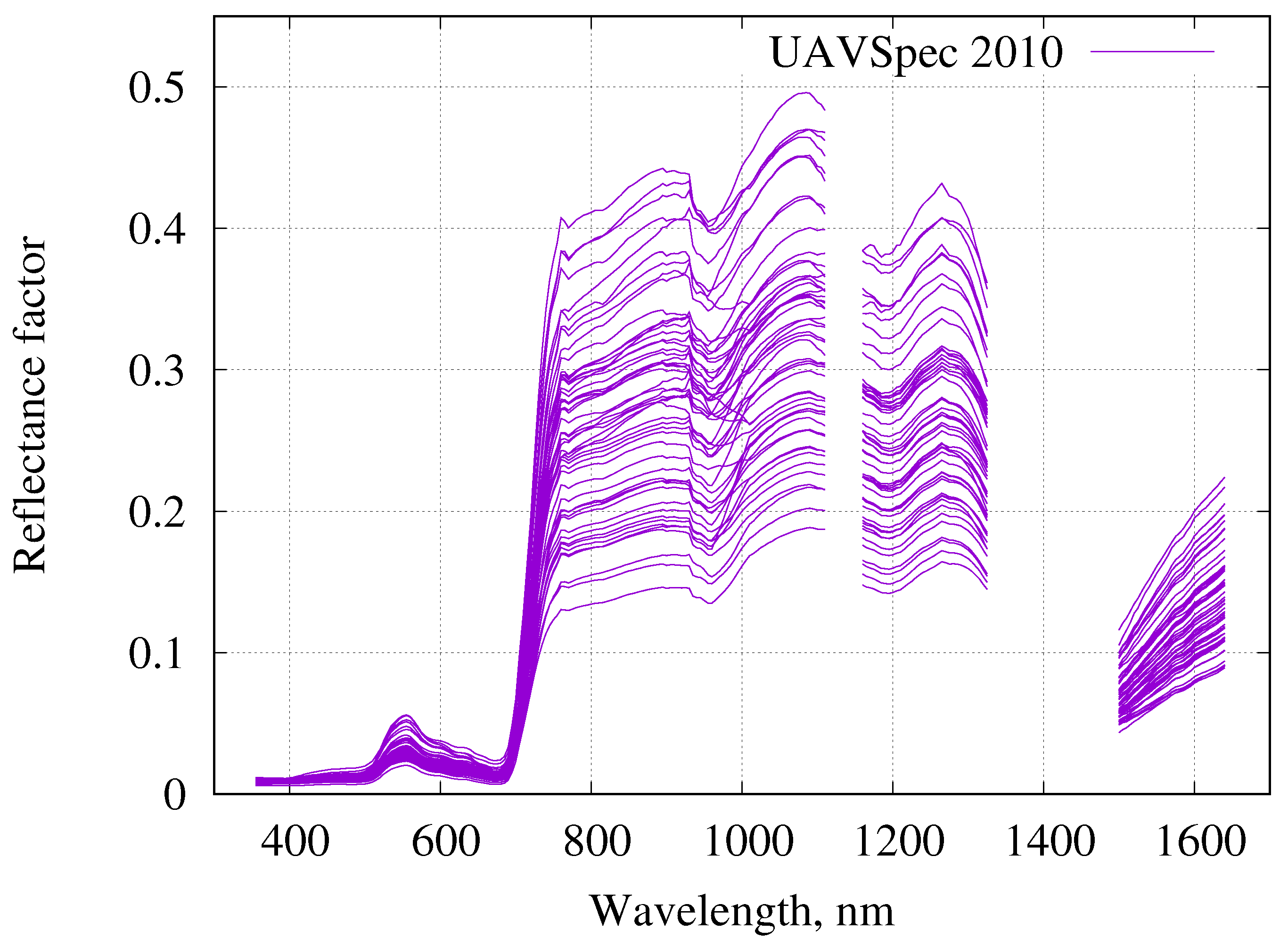
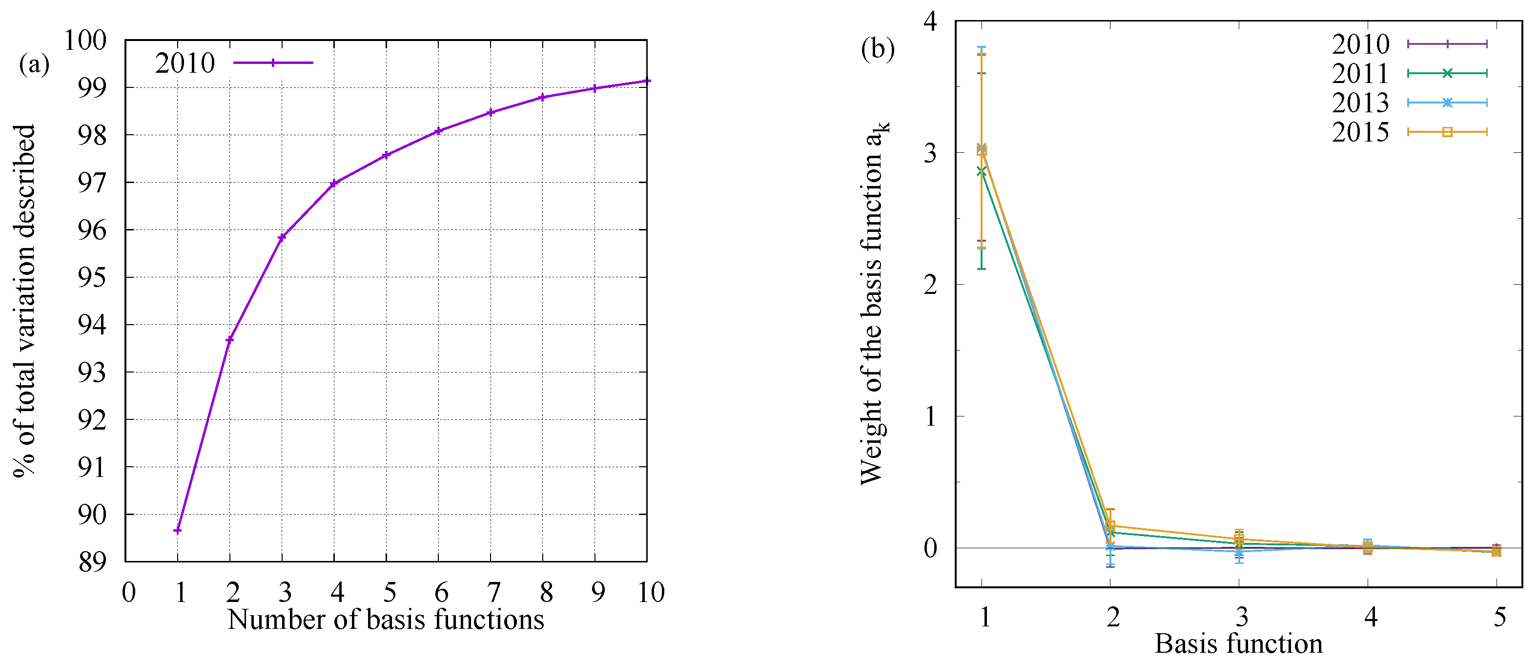
The following analysis uses those stands for which at least 10 VisNIR spectra were recorded. The range of the number of recorded spectra over a stand varied in general from 10 to 130. Exceptions were three mature stands, over which several passes were made, raising the number of spectra recorded to 1300. Spectra recorded in the buffer zone of 8 m at the stand borders were not involved. Clear-cut areas and stands younger than 5 years were removed from the current analyses. The average spectrum of the directional reflectance factor for every stand was calculated. A total of 578 stands was involved. Measured spectra of 2010 are plotted in Figure 2.

Recorded spectra can be presented as a linear combination of arbitrary fixed functions $X_k\left(\lambda \right)$ of wavelength $\lambda$,

$$\rho \left(\lambda \right)=\sum _{k=1}^n{a}_k{X}_k\left(\lambda \right),$$

(2)

where $\rho \left(\lambda \right)$ is the directional reflectance factor, $X_k\left(\lambda \right)$ are called basis functions, and $a_k$ is the weight of the basis function $X_k\left(\lambda \right)$ [12]. The basis functions were found with general linear least squares [12]. As the range of reflectance values was large, extending from a few percent in blue and red light to almost 50% in NIR, the merit function ${\chi }^2$ for least squares was normalized by the standard deviation of reflectance values,

$${\chi }^2=\sum _j{\left(\frac{\rho \left({\lambda }_j\right)-{\sum }_k{a}_k{X}_k\left({\lambda }_j\right)}{{\sigma }_j}\right)}^2,$$

(3)

where ${\sigma }_j$ is the standard deviation of directional reflectance factor at wavelength ${\lambda }_j$. The procedure of singular value decomposition [12] was used for solving the problem of least squares.

3. Results

3.1. Basis Functions

The first five basis functions are plotted in Figure 3. The interpretation of the basis functions is straightforward. The first basis function describes the average shape of the reflectance spectrum, and varying the weight of this basis function sets the level of reflectance. The other basis functions describe the deviations of the spectrum shape from the average spectrum, caused by the variations in the stand properties (age, stand density, species composition, foliage pigments, site type, canopy structure, etc.). Basis function were found separately for every year, and for the whole set of 1233 spectral signatures. The first four basis functions almost coincide in different years. Only the basis functions of 2015 deviate from others. Only 42% of stands were measured in 2015, and due to changing weather, the spectral distribution of incident radiation at every stand could deviate from that at supporting spectrometer at the distance of 2–5 km. The spectral profile of the fifth basis function varies dependent on the subset of stands involved.

Figure 4a shows that the first five basis functions describe almost 98% of variance of reflectance spectra measured over more than 350 stands on 5 July 2010. The weight of the first basis function is positive, and varies from stand to stand in rather large range (Figure 4b). The weights of subsequent basis functions may be either positive or negative, and are in absolute value, significantly less than the weight of the first basis function. Figure 5 shows that forest reflectance spectra are represented with high precision if five basis functions are used in the linear combination Equation (2).

3.2. Weights of Basis Functions

The weights of basis functions $a_k$ for constructing Figure 5 were found with linear least squares by optimizing Equation (3). In order to find how the weights $a_k$ are related to forest parameters, the stands were separated into three groups: spruce stands, pine stands, and broadleaf stands. The multiple regression between 15 primary inventory parameters and weights $a_k$ was found (

Table 2. Multiple correlation of inventory parameters and weights of basis functions.

Weight	Pine Forests	Spruce Forests	Broadleaf Forests
$a_1$	0.870	0.720	0.679
$a_2$	0.921	0.653	0.451
$a_3$	0.885	0.447	0.478
$a_4$	0.764	0.710	0.579
$a_5$	0.712	0.656	0.443

). Multiple correlation describes a dependent variable in case of multiple predictors [19]. Calculations were carried out in the spreadsheet Gnumeric [20].

3.3. Statistical Forest Reflectance Model (SFRM)

The spectral reflectance of a forest stand (presented in vector form) can be estimated with the help of basis functions and regression between inventory parameters and the weights of basis functions as

$$\mathcal{R}=\mathcal{A}\times \mathcal{X},$$

(4)

where $\mathcal{R}$, $\mathcal{A}$, and $\mathcal{X}$ are the vectors of spectral reflectances and weights, and the matrix of basis functions, respectively. The elements of the vector $\mathcal{A}$ are calculated as the multiple regression of forest inventory parameters, as

$$a_k=\sum _{j=1}^{15}{r}_{jk}{\gamma }_j+b_{j1},$$

(5)

where $r_{jk}$ are the coefficients of multiple regression, ${\gamma }_j$ are the forest inventory parameters, and $b_{j1}$ is the intercept of the regression line for the first weight $a_1$. For finding the weights of other basis functions, the intercept of the regression line was constrained to be zero.

3.4. Validation of the Model

Validation of the model was carried out in two steps. First, the simulated spectra were compared with the recorded spectra from helicopter measurements in July 2010. Forest inventory data of 2011 were used as the input to the SFRM. The mean relative error $(\langle {\rho }_s\left(\lambda \right)\rangle -\langle {\rho }_m\left(\lambda \right)\rangle )/\langle {\rho }_m\left(\lambda \right)\rangle$ was calculated for every stand, using spectra recorded on 5 July 2010 (where the subscripts s and m denote simulated and measured values, respectively, and the angle brackets $\langle \rangle$ denote mean averaging over a stand). Measured and simulated spectra at 217 wavelengths over 45 pine, 59 spruce, and 231 broadleaf stands were compared. The histograms of relative errors for the three groups of stands are plotted in Figure 6, Figure 7 and Figure 8.

The validation confirmed that the predicted reflectance had no systematic errors. The random relative errors lay mostly within the 0–15% range. The error exceeded 30% for only 6 stands out of 335. This could be due to inhomogeneities within stands, with the flight transect crossing some nontypical part of a stand. Forest inventory data describe average parameter values of the whole stand.

The second validation was done using data from the Sentinel-2B acquisition over the test site on 18 August 2019. Figure 9 presents the test site in band 7 (780 nm) of the Multispectral Imager (MSI). The perimeter of the forest district, and additionally the stand borders, are marked in brown. The blue rectangle marks the excerpt in Figure 1. Atmospheric correction of the level 1C images, bands 2–11, was performed with the method suggested by Kuusk et al. [21]. Atmospheric optical parameters were estimated using the irradiance spectra from the simultaneous measurements with the spectrometer SkySpec at the test site [22,23]. Spectral images of the 20 m spatial resolution bands B5, B6, B7, B8a, and B11 were resampled to 10 m resolution, using the bicubic upsampling method in the Sentinel-2 Toolbox [24]. Spectral signatures of 514 spruce stands, 601 pine stands, and 2121 broadleaf stands, altogether 3236 stands, were measured from the spectral images. Forest stands were selected by requiring the age of the dominant species to be greater than 5 years and the stand image to enclose at least ten 10 m × 10 m pixels. It was additionally required that the center of each selected pixel be at least 8 m from the stand border. The average area of the stands meeting these criteria was 1.72 ha, the smallest and largest areas being 0.2 ha and 42 ha.

The distribution of relative errors for the three groups of stands is plotted in Figure 10, Figure 11 and Figure 12 and tabulated in

Table 3. Mean relative errors of simulated reflectance, and their standard deviations (STDs).

	Spruce Forest		Pine Forest		Broadleaf Forest
Band	Mean	STD	Mean	STD	Mean	STD
B2 (492 nm)	−0.196	0.163	−0.247	0.147	−0.153	0.143
B3 (559 nm)	−0.028	0.182	−0.082	0.221	0.033	0.153
B4 (665 nm)	−0.206	0.200	−0.204	0.246	−0.211	0.180
B5 (704 nm)	0.073	0.212	0.040	0.290	0.132	0.169
B6 (739 nm)	0.049	0.230	0.017	0.543	0.166	0.127
B7 (780 nm)	0.023	0.234	0.006	0.577	0.154	0.130
B8 (833 nm)	0.096	0.247	0.069	0.614	0.191	0.134
B8a (864 nm)	−0.033	0.220	−0.041	0.548	0.085	0.119
B11 (1610 nm)	0.008	0.277	0.045	0.387	0.098	0.146
All bands	−0.024	0.243	−0.044	0.444	0.055	0.199

. The range of errors is rather equal in spruce and broadleaf stands, with the standard deviation lying between 0.12 and 0.28. There are two reasons for the higher dispersion of simulation errors in pine stands. The selection of pine stands which were used for calculating the basis functions was not so representative as that of broadleaf and spruce stands. Additionally, there are 15 stands where the main species is pine, but the total share of broadleaf species (birch, alder, and aspen) is close to, or even exceeds, the share of pine trees. In these stands, the large contribution from broadleaf species substantially modifies the spectral signature from pine. Shuch stands could be considered broadleaf.

Systematic errors in the simulated spectra are greatest in the dark bands B2 and B4 (blue and red), where the role of the atmosphere in the satellite signal is substantial. Possible small errors in optical parameter values of the atmosphere result in erroneous atmospheric correction of satellite images, yielding systematically biased ground reflectance values in these spectral bands. While the relative errors are in the range from 20% to 40–50%, the mean differences of reflectance values are very small (Figure 13). Only the NIR reflectance of broadleaf stands is overestimated by 0.02–0.05, on average. The same order of differences between simulated forest reflectance was observed with radiation transfer model intercomparison (RAMI), where participating models simulated directional spectral reflectance of a few forest stands which were described in full detail [3].

4. Discussion

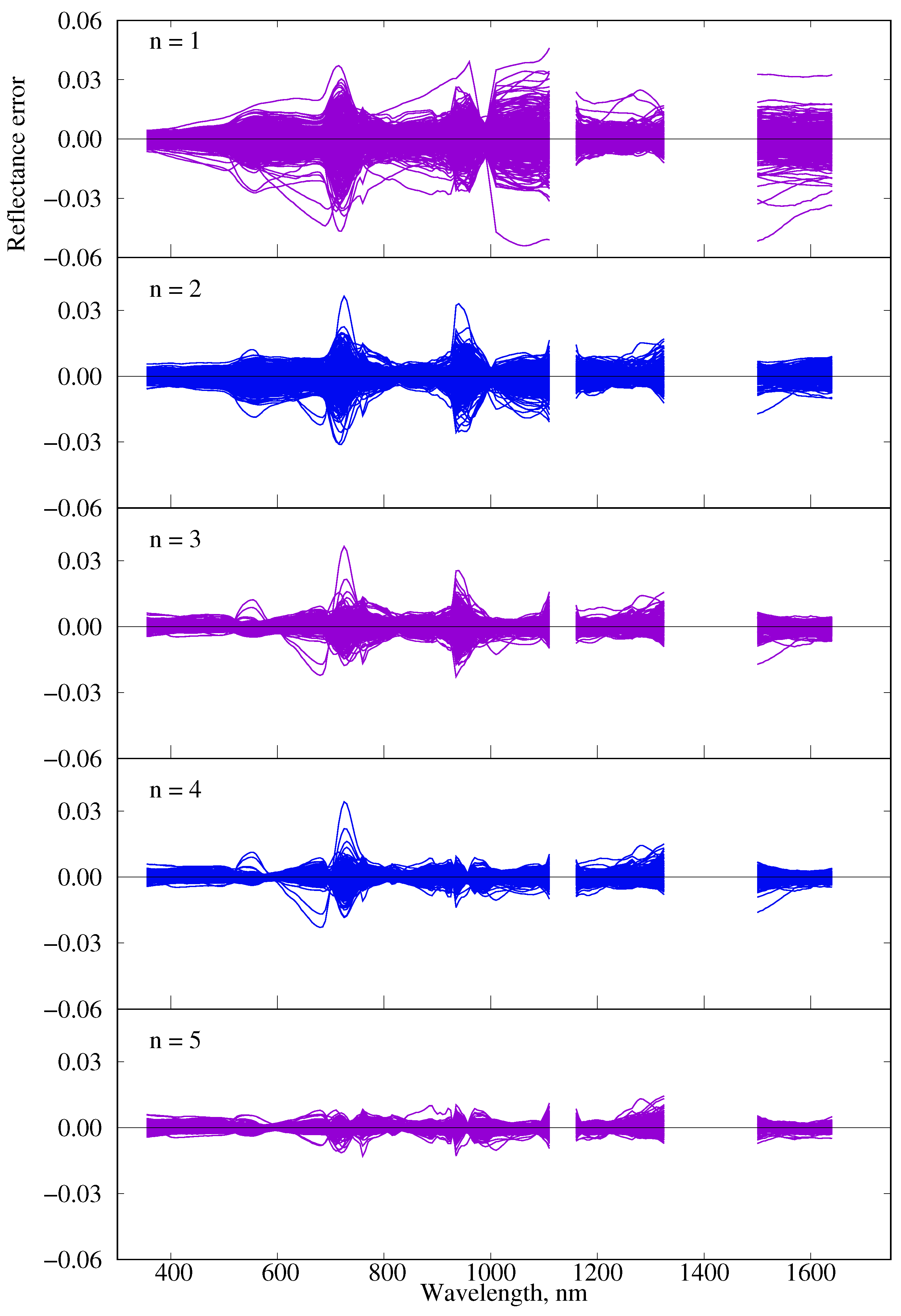
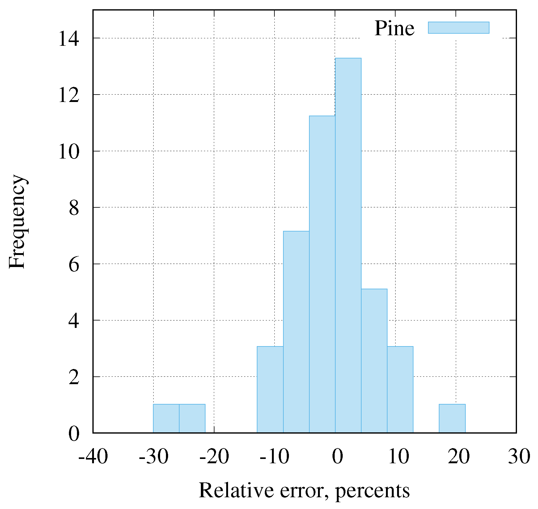
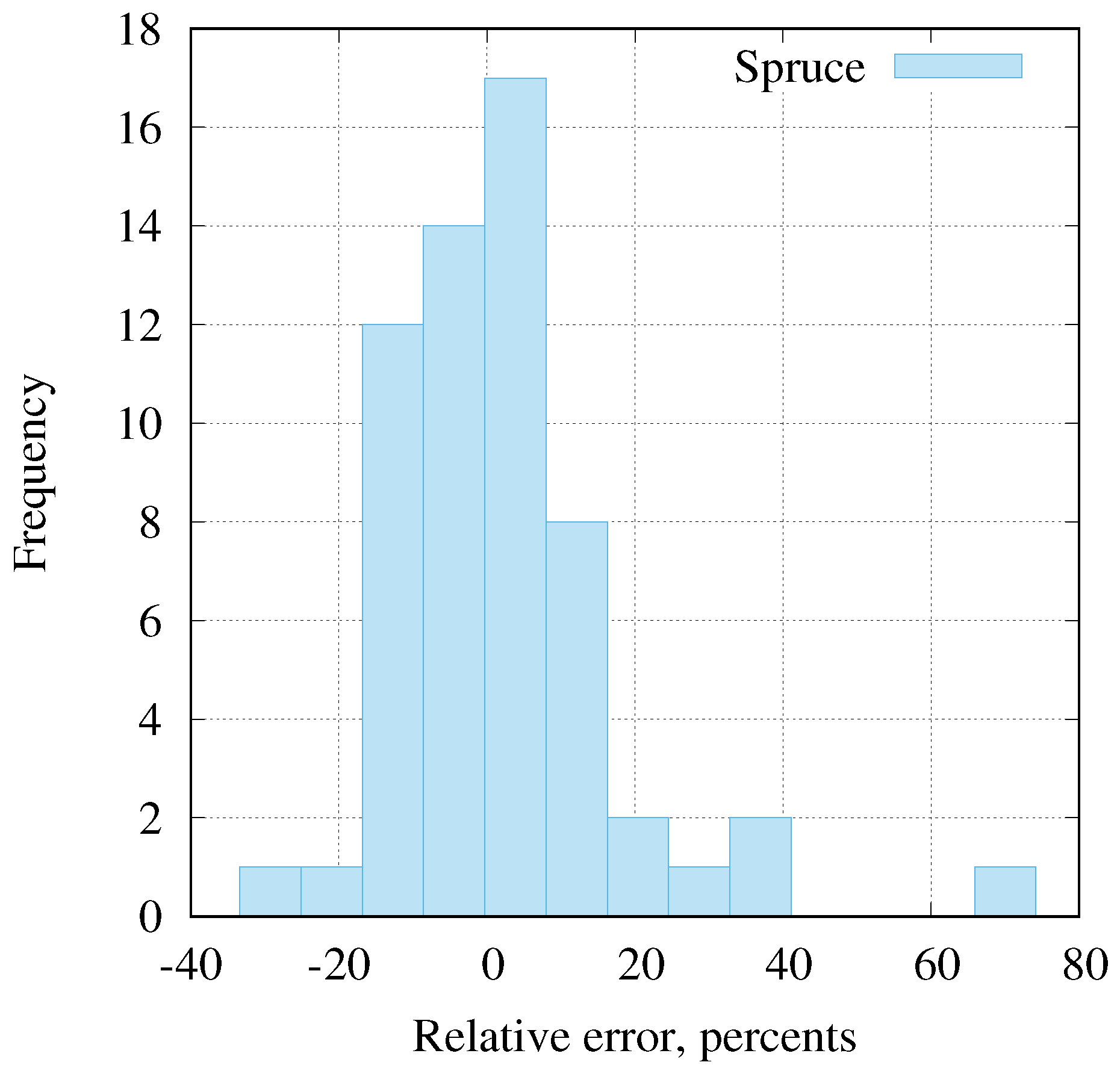
Despite the high diversity of forests, the reflectance spectra of hemiboreal forests do not vary greatly. We showed that the variability of reflectance spectra can be well described with five basis functions in the visible-NIR-SWIR spectral domain. Reflectance spectra can be predicted with a statistical model as the linear combination of basis functions where the weights of basis functions are statistically related to the forest inventory parameters. In this way the stand reflectance spectrum is predicted from information available in the forest management inventory database. In the provided model, the 15 primary inventory parameters are used as the independent predictors. The 15 parameters are of course not all equally significant. It would, in principle, be possible to predict the reflectance of a stand using only significant predictors. However, the set of significant predictors not only is different for stands of different dominant species (pine, spruce, and broadleaf) but also varies between the weights $a_k$ of different basis functions for the same type of forest. At the same time, all these stand parameters are, in any case, recorded in the course of regular forest inventory. Therefore, all the 15 primary parameters were used in the multiple regressions of all species and for all the weights of basis functions in the model SFRM.

The reflectance model makes it possible to estimate directional reflectance spectra and albedo of forests which are covered by forest management inventory databases. Such information is required in models of the landscape energy budget, in primary production estimation, and in complex studies of forested environment at stations for measuring ecosystem-atmosphere relations (SMEAR) [25,26].

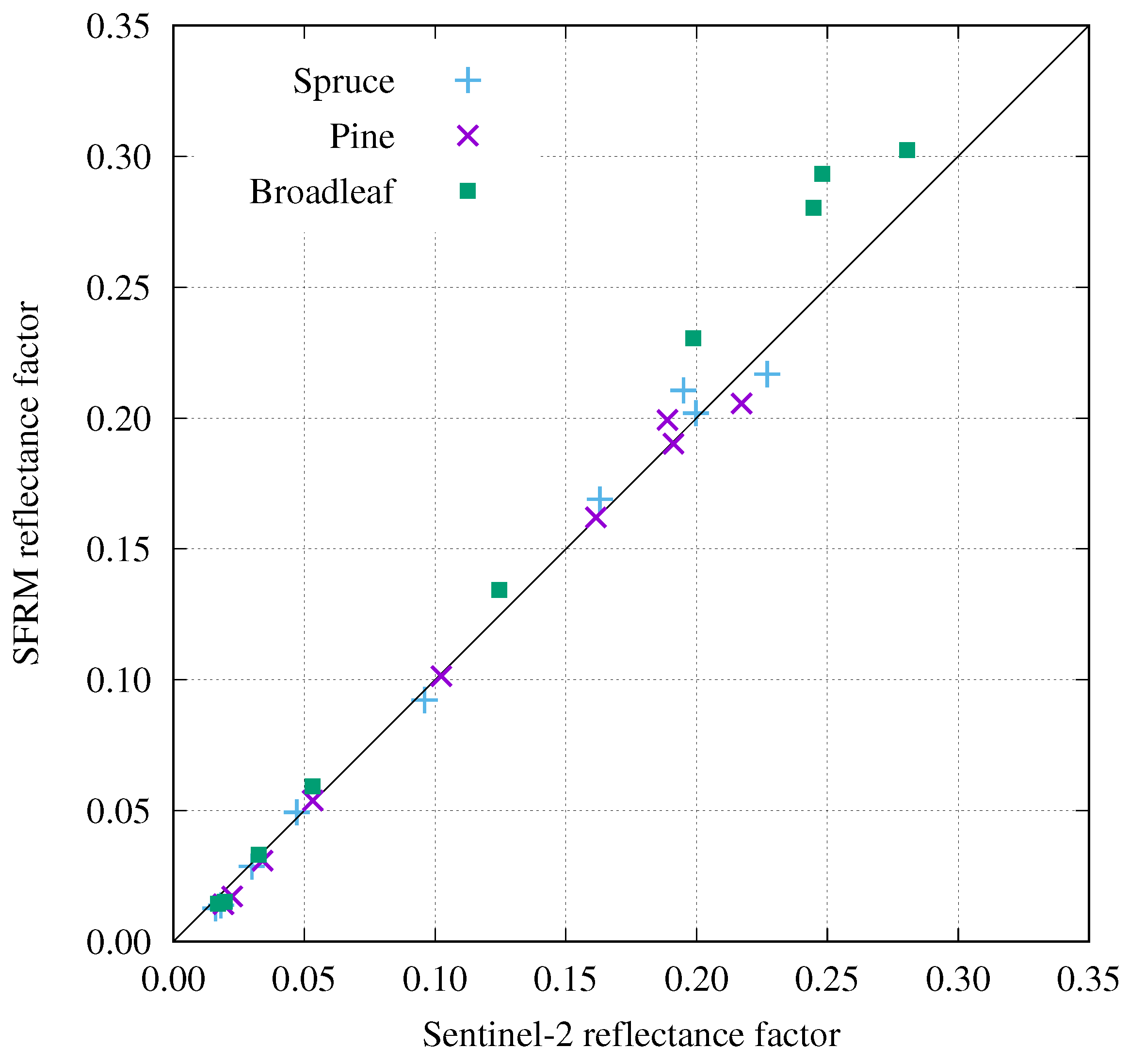
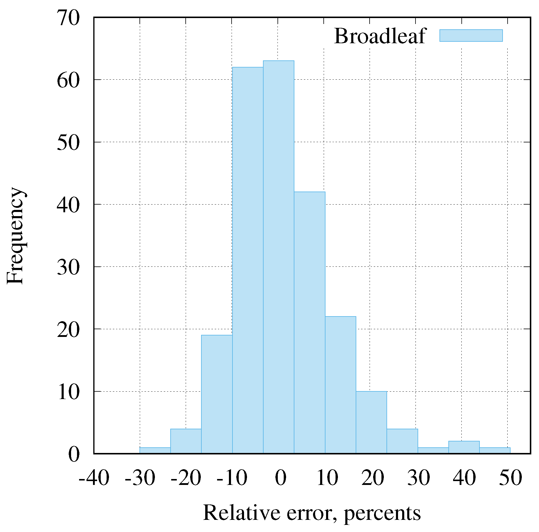
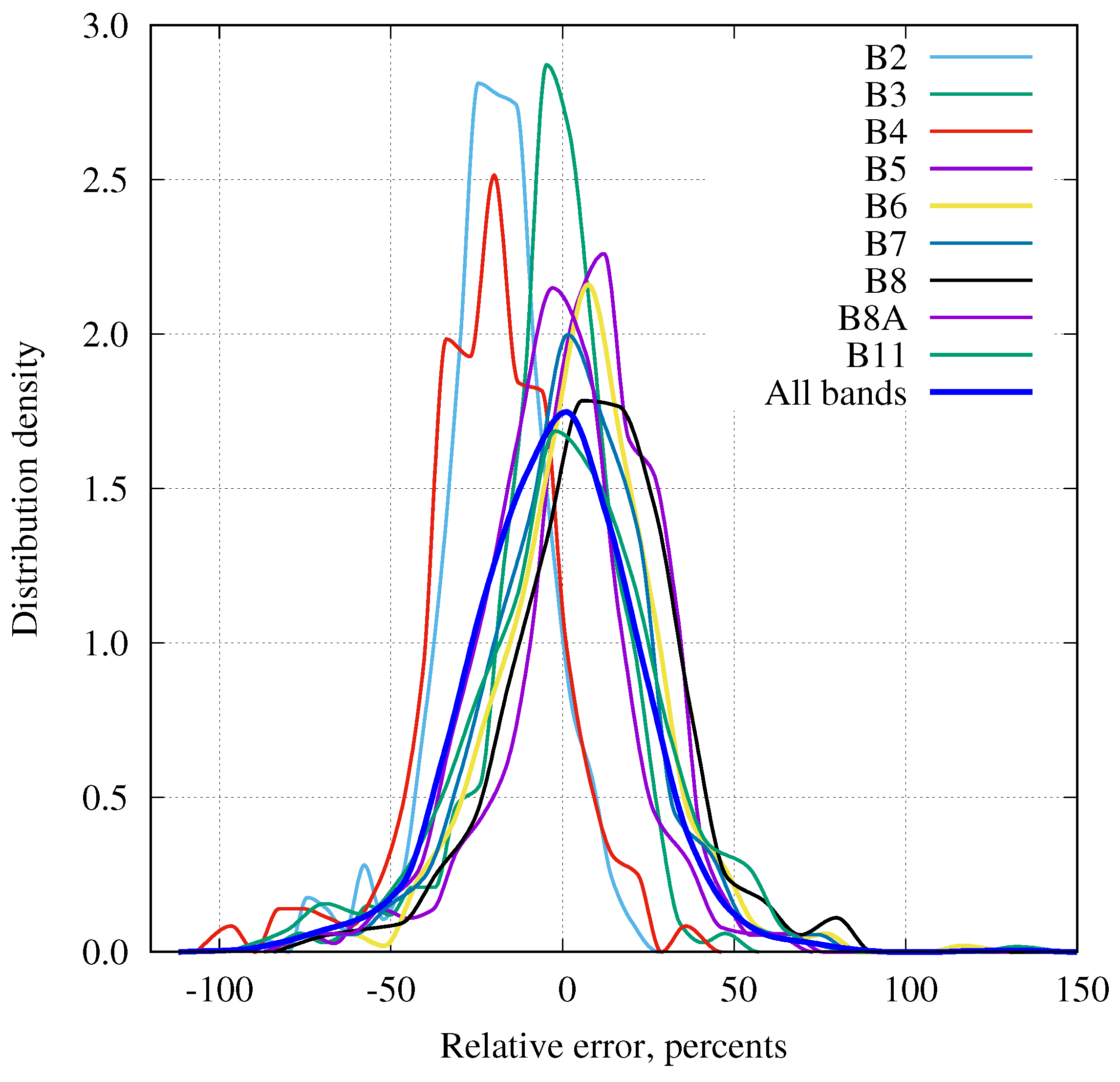
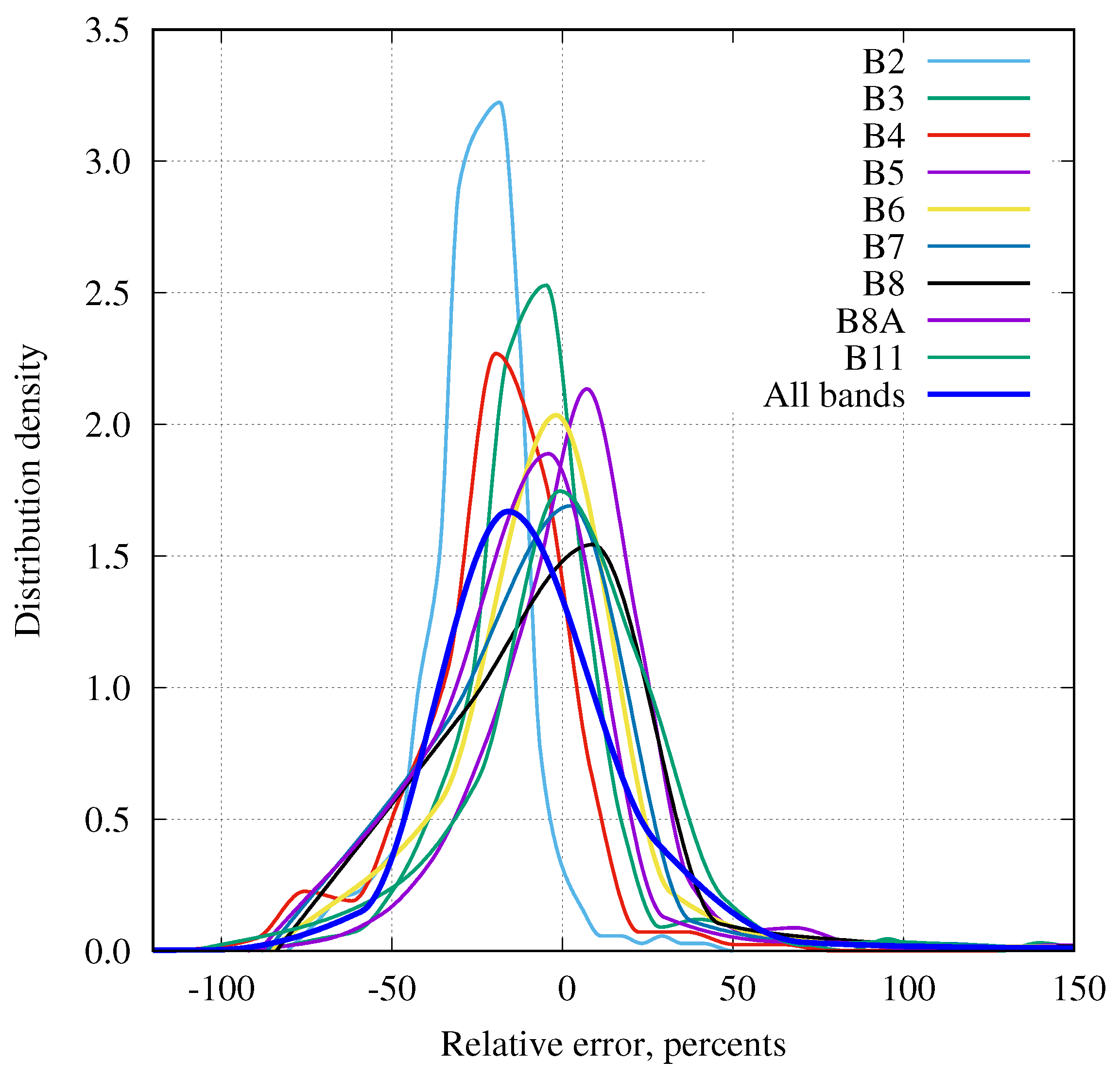
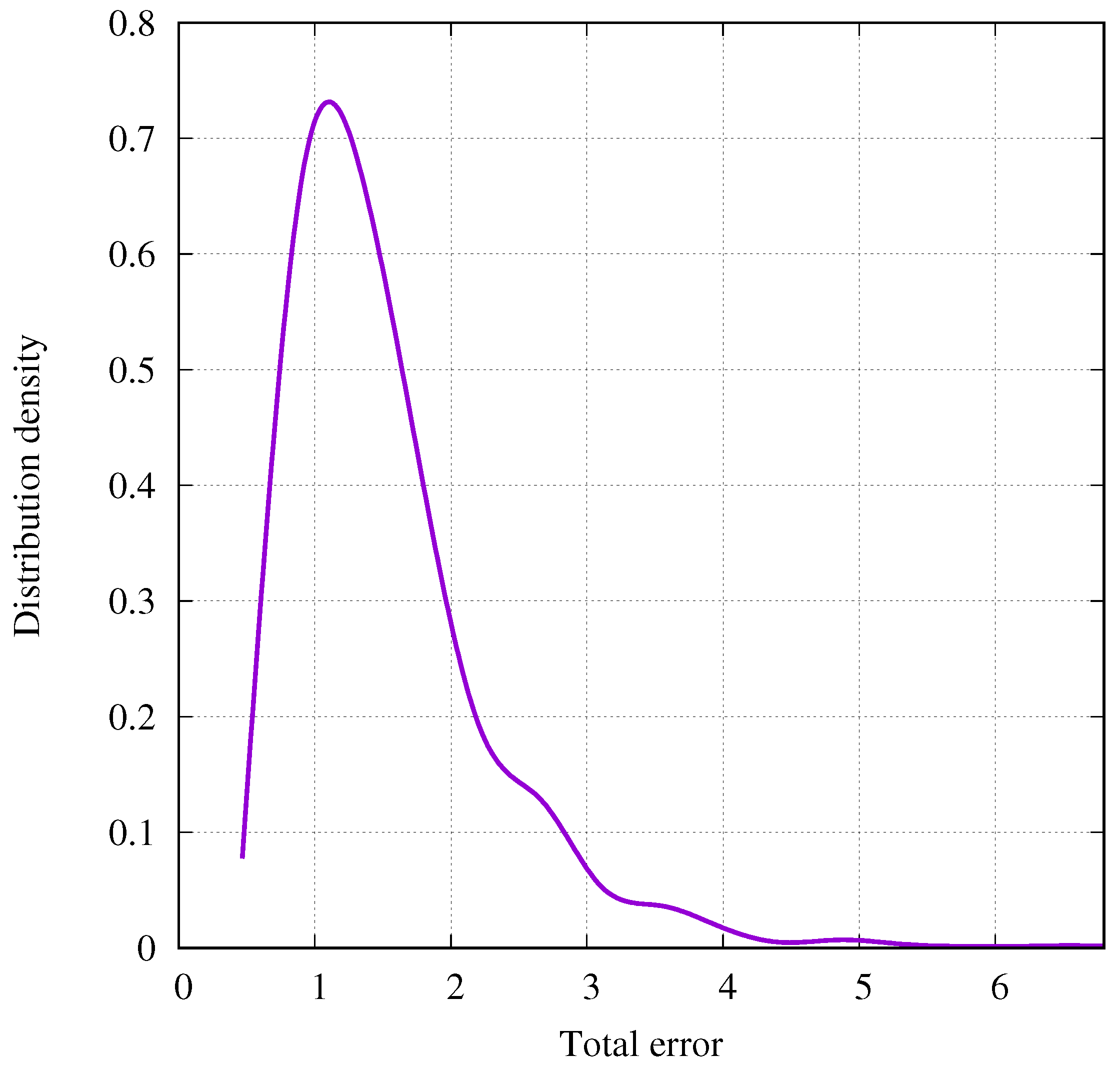
Comparison of simulated reflectance to satellite data at comparable respective spatial resolutions (as with Sentinel-2 MSI and Landsat TM) may be used for finding errors in stand inventory records. This idea has indeed already been suggested by Nilson et al. [8]. Figure 14 shows the distribution of the total error S of simulated spectra for Sentinel-2 MSI spectral bands, taken as

$$\begin{array}{c}\hfill S={\displaystyle \sum _{j=B2}^{B11}}\frac{|\langle {\rho }_s\left({\lambda }_j\right)\rangle -\langle {\rho }_m\left({\lambda }_j\right)\rangle |}{\langle {\rho }_m\left({\lambda }_j\right)\rangle }.\end{array}$$

(6)

A high value of the error S serves as an indicator to forest managers that the inventory data of the pertinent stands could be erroneous or outdated, giving those data points priority in their checking process.

With this model, the inverse problem, namely, the estimating of forest parameters from top-of-canopy reflectance data, is problematic. The difficulty stems from a double linear combination, with the weighted summation of basis functions using weights that are themselves in turn the weighted sums of forest inventory parameters. Jakubauskas and Price [27] have made an attempt to estimate stand structure parameters of lodgepole pine forests as the multiple regression of Landsat-5 TM reflectance values in optical bands. While some stand parameters were predictable from remotely sensed data, factors relating specifically to understory condition were poorly predicted by spectral data, even with the inclusion of data transformations or indices. Data transformations (e.g., NDVI and Tasseled Cap) provided some measure of data reduction, but did not substantially increase the strength of the statistical relationship between spectral and biotic variables. Estimating forest inventory parameters by the inversion of the SFRM model is ill-posed; the number of forest inventory parameters exceeds the number of independent model parameters needed for the simulation of forest reflectance. Therefore, only a few of the most significant model parameters can be estimated in an inversion.

As with every regression model, this model works only in environmental and geographical conditions which are similar to the training observations. The basis functions and regression coefficients in this work were found using spectral signatures of hemiboreal forests. The same procedure can be applied in different conditions if data from National Forest Inventory or regular forest management inventory database, and high quality spectral signatures for developing basis functions are available.

5. Conclusions

A simple statistical model for the simulation of forest directional reflectance spectra was provided. The input parameters of the model are the forest parameters collected by forest managers. The simulated reflectance spectra were found to be in good agreement with measured spectra. In most cases the relative difference did not exceed 10–15%; only a few exceptions had the error more than 30%. The model is computationally very simple and fast. The estimation of forest parameters through inversion of the model is, however, problematic, due to the two-stage linear combination on which the model is founded.

References

1. Goel, N. Models of vegetation canopy reflectance and their use in estimation of biophysical parameters from reflectance data. Remote Sens. Rev. 1988, 4, 1–212. [Google Scholar] [CrossRef]
2. Pinty, B.; Gobron, N.; Widlowski, J.L.; Gerstl, S.A.; Verstraete, M.M.; Antunes, M.; Bacour, C.; Gaston, F.; Gastellu, J.P.; Goel, N.; et al. Radiation transfer model intercomparison (RAMI) exercise. J. Geophys. Res. D Atmos. 2001, 106, 11937–11956. [Google Scholar] [CrossRef]
3. Widlowski, J.L.; Mio, C.; Disney, M.; Adams, J.; Andredakis, I.; Atzberger, C.; Brennan, J.; Busetto, L.; Chelle, M.; Ceccherini, G.; et al. The fourth phase of the radiative transfer model intercomparison (RAMI) exercise: Actual canopy scenarios and conformity testing. Remote Sens. Environ. 2015, 169, 418–437. [Google Scholar] [CrossRef]
4. Kuusk, A. Canopy radiative transfer modeling. In Comprehensive Remote Sensing. V. 3, Terrestrial Ecosystems; Liang, S., Ed.; Elsevier: Oxford, UK, 2018; pp. 9–22. [Google Scholar]
5. Liang, S. Quantitative Remote Sensing of Land Surfaces; Wiley-Interscience: Hoboken, NJ, USA, 2004. [Google Scholar]
6. Burkhart, H.; Tomé, M. Modeling Forest Trees and Stands; Springer: Dordrecht, The Netherlands, 2012. [Google Scholar]
7. Ferretti, M.; Fisher, R. (Eds.) Forest Monitoring. Methods for Terrestrial Investigations in Europe with an Overview of North America and Asia; Elsevier: Oxford, UK, 2013. [Google Scholar]
8. Nilson, T.; Lang, M.; Kuusk, A.; Anniste, J.; Lükk, T. Forest reflectance model as an interface between satellite images and forestry databases. In Remote Sensing and Forest Monitoring; Zawila-Niedzwiecki, T., Brach, M., Eds.; Office for Official Publications of the European Communities: Luxembourg, 2000; pp. 462–476. [Google Scholar]
9. White, J.; Gómez, C.; Wulder, M.; Coops, N. Characterizing temperate forest structural and spectral diversity with Hyperion EO-1 data. Remote Sens. Environ. 2010, 114, 1576–1589. [Google Scholar] [CrossRef]
10. Coppo, P.; Taiti, A.; Pettinato, L.; Francois, M.; Taccola, M.; Drusch, M. Fluorescence imaging spectrometer (FLORIS) for ESA FLEX mission. Remote Sens. 2017, 9, 649. [Google Scholar] [CrossRef]
11. Kuusk, J.; Kuusk, A. Autonomous lightweight airborne spectrometers for ground reflectance measurements. In Proceedings of the 2nd Workshop on Hyperspectral Image and Signal Processing: Evolution in Remote Sensing (WHISPERS 2010), Reykjavik, Iceland, 14–16 June 2010. [Google Scholar]
12. Press, W.; Teukolsky, S.; Vetterling, W.; Flannery, B. Numerical Recipes in FORTRAN. The Art of Scientific Computing; Cambridge University Press: Cambridge, UK, 1992. [Google Scholar]
13. Price, J. On the information content of soil reflectance spectra. Remote Sens. Environ. 1990, 33, 113–121. [Google Scholar] [CrossRef]
14. Forest inventory act (Metsa korraldamise juhend). In Riigi Teataja; RT I, 24.11.2015, 6; Official Publication by the Government of Estonia: Tallinn, Estonia, 2015.
15. Kuusk, A.; Lang, M.; Nilson, T. Forest test site at Järvselja, Estonia. In Proceedings of the Third Workshop CHRIS/Proba, Frascati, Italy, 21–23 March 2005; ESA Publication SP-593. pp. 1–7. [Google Scholar]
16. Kuusk, J. Dark signal temperature dependence correction method for miniature spectrometer modules. J. Sens. 2011, 2011, 1–9. [Google Scholar] [CrossRef]
17. Kostkowski, H.J. Reliable Spectroradiometry; Spectroradiometry Consulting: La Plata, MD, USA, 1997. [Google Scholar]
18. Kuusk, J.; Ansko, I.; Bialek, A.; Vendt, R.; Fox, N. Implication of illumination beam geometry on stray light and bandpass characteristics of diode array spectrometer. IEEE J. Sel. Top. Appl. Earth Obs. Remote Sens. 2018, 11, 2925–2932. [Google Scholar] [CrossRef]
19. Klugh, H. Statistics: The Essentials for Research; Wiley: New York, NY, USA, 1974. [Google Scholar]
20. Gnumeric. Gnumeric Spreadsheet. Available online: http://gnumeric.org (accessed on 9 August 2019).
21. Kuusk, A.; Kuusk, J.; Lang, M.; Lükk, T. Vicarious calibration of the PROBA/CHRIS imaging spectrometer. Photogramm. J. Finl. 2010, 22, 46–59. [Google Scholar]
22. Kuusk, J.; Kuusk, A. Hyperspectral radiometer for automated measurement of global and diffuse sky irradiance. J. Quant. Spectrosc. Radiat. Transf. 2018, 204, 272–280. [Google Scholar] [CrossRef]
23. Kuusk, A.; Kuusk, J. Estimation of variable atmospheric parameters for the atmospheric correction of satellite images. Int. J. Remote Sens. 2018, 39, 565–576. [Google Scholar] [CrossRef]
24. ESA. The Sentinel-2 Toolbox. Available online: https://sentinel.esa.int/web/sentinel/toolboxes/sentinel-2 (accessed on 15 October 2019).
25. Noe, S.; Niinemets, U.; Krasnova, A.; Krasnov, D.; Motallebi, A.; Kängsepp, V.; Jõgiste, K.; Hõrrak, U.; Komsaare, K.; Mirme, S.; et al. SMEAR Estonia: Perspectives of a large-scale forest ecosystem – atmosphere research infrastructure. For. Stud. 2015, 63, 56–84. [Google Scholar] [CrossRef]
26. Lappalainen, H.; Kerminen, V.M.; Petäjä, T.; Kurten, T.; Baklanov, A.; Shvidenko, A.; Bäck, J.; Vihma, T.; Alekseychik, P.; Andreae, M.O.; et al. Pan-Eurasian Exp. (PEEX): Towards A Holist. Underst. Feed. Interact. Land–atmosphere–ocean–society Contin. North. Eurasian Reg. Atmos. Chem. Phys. 2016, 16, 14421–14461. [Google Scholar] [CrossRef] [Green Version]
27. Jakubauskas, M.; Price, K. Empirical relationships between structural and spectral factors of Yellowstone lodgepole pine forests. Photogramm. Eng. Remote Sens. 1997, 63, 1375–1381. [Google Scholar]
Figure 1. Flight route of helicopter measurements on 5 July 2010, with forest stand borders. The background is the satellite image of Proba/CHRIS scene DD40 band 12 (NIR) of 27 July 2011, at a spatial resolution of 17 m. Yellow polygons mark the stands involved in this study, and the red cross marks the place of incident radiation measurement.
Remotesensing 11 02749 g001
Figure 2. Reflectance spectra of forest stands on 5 July 2010.
Remotesensing 11 02749 g002
Figure 3. Basis functions for the forest directional reflectance factor. Gaps in data are due to weak signal in the absorption bands of water vapor in the atmosphere.
Remotesensing 11 02749 g003
Figure 4. Cumulative percentage of variance described by basis functions (a), and mean value and standard deviation of the weights of basis functions (b).
Remotesensing 11 02749 g004
Figure 5. Error of the representation of forest spectra as a function of the number n of basis functions in Equation (2).
Remotesensing 11 02749 g005
Figure 6. Relative errors of simulated spectra, pine stands.
Remotesensing 11 02749 g006
Figure 7. Relative errors of simulated spectra, spruce stands.
Remotesensing 11 02749 g007
Figure 8. Relative errors of simulated spectra, broadleaf stands.
Remotesensing 11 02749 g008
Figure 9. Sentinel-2 MSI image B7 (780 nm) of the test site on 18 August 2019. Brown lines mark the contours of the forest district and of the individual stands. The blue rectangle marks the region of Figure 1.
Remotesensing 11 02749 g009
Figure 10. Relative errors of simulated spectra, spruce stands.
Remotesensing 11 02749 g010
Figure 11. Relative errors of simulated spectra, pine stands.
Remotesensing 11 02749 g011
Figure 12. Relative errors of simulated spectra, broadleaf stands.
Remotesensing 11 02749 g012
Figure 13. Mean reflectance factors in Sentinel-2 MSI spectral bands and the simulation with the statistical forest reflectance model (SFRM).
Remotesensing 11 02749 g013
Figure 14. Distribution of the total error, Equation (6).
Remotesensing 11 02749 g014