Deep Learning-Generated Nighttime Reflectance and Daytime Radiance of the Midwave Infrared Band of a Geostationary Satellite


Abstract
1. Introduction
2. Data
3. Method
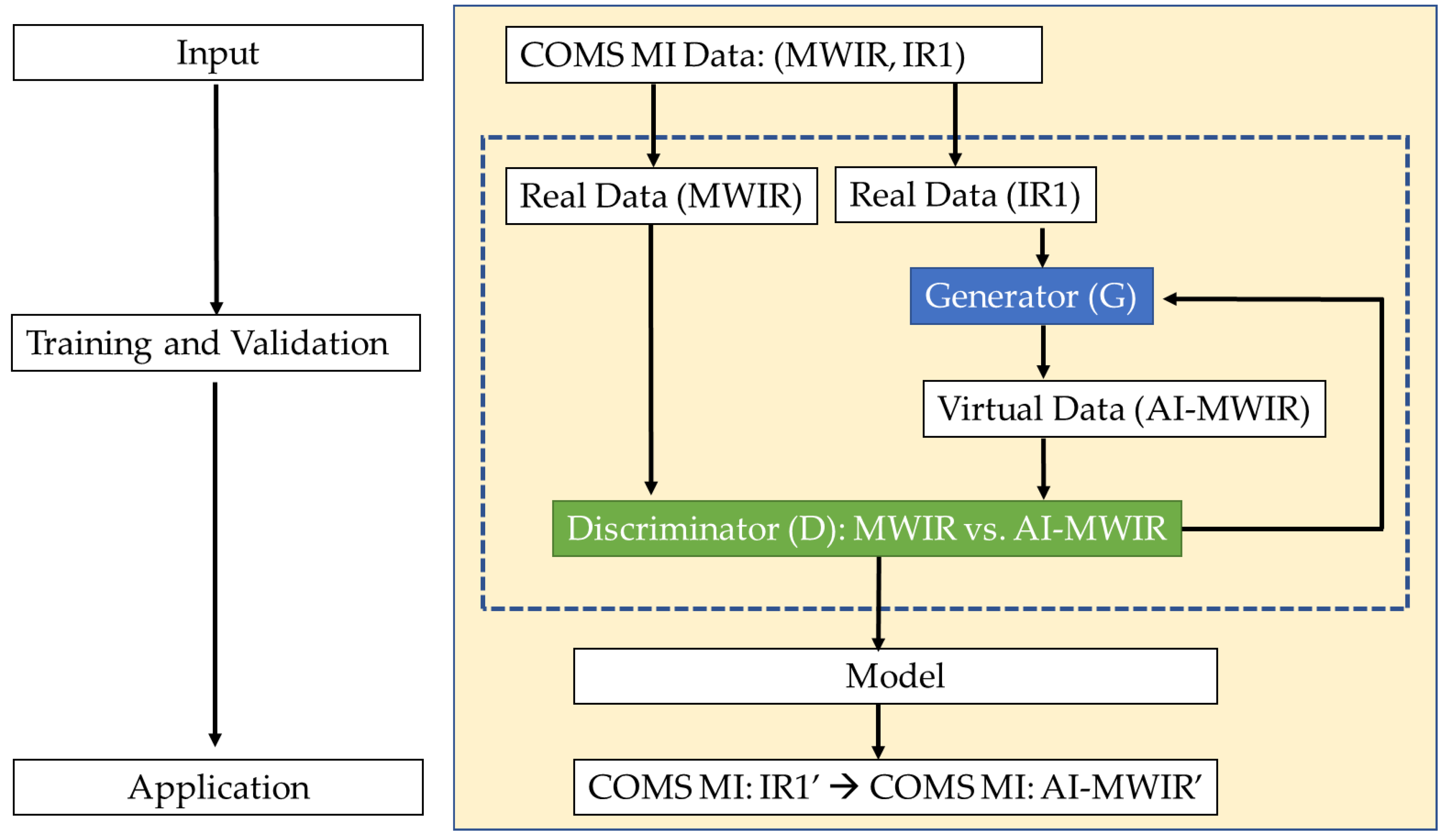
3.1. CGAN
3.2. Band Selection for CGAN
3.3. Implementation
4. Results
5. Discussion
6. Summary and Concluding Remarks
Author Contributions
Funding
Acknowledgments
Conflicts of Interest
References
- Escrig, H.; Batlles, F.J.; Alonso, J.; Baena, F.M.; Bosch, J.L.; Salbidegoitia, I.B.; Burgaleta, J.I. Cloud detection, classification and motion estimation using geostationary satellite imagery for cloud cover forecast. Energy 2013, 55, 853–859. [Google Scholar] [CrossRef]
- Purdom, J.; Menzel, P. Evolution of Satellite Observation in the United States and Their Use in Meteorology. In Historical Essays on Meteorology 1919–1995; Fleming, J.R., Ed.; American Meteorological Society: Boston, MA, USA, 1996; pp. 99–156. [Google Scholar]
- Schmetz, J.; Pili, P.; Tjemkes, S.; Just, D.; Kerkmann, J.; Rota, S.; Ratier, R. Supplement to an introduction to Meteosat Second Generation (MSG). Bull. Am. Meteorol. Soc. 2002, 83, 991. [Google Scholar] [CrossRef]
- Yusuf, A.A.; Francisco, H. Climate Change Vulnerability Mapping for Southeast Asia. Economy and Environment Program for Southeast Asia (EEPSEA), Singapore with CIDA, IDRC and SIDA. 2009. Available online: https://www.idrc.ca/sites/default/files/sp/Documents%20EN/climate-change-vulnerability-mapping-sa.pdf (accessed on 23 September 2019).
- Schmit, T.J.; Gunshor, M.M.; Menzel, W.P.; Gurka, J.J.; Li, J.; Bachmeier, A.S. Introducing the next-generation advanced baseline imager on GOES-R. Bull. Am. Meteorol. Soc. 2005, 86, 1079–1096. [Google Scholar] [CrossRef]
- Bessho, K.; Date, K.; Hayashi, M.; Ikeda, A.; Imai, T.; Inoue, H.; Kumagai, Y.; Miyakawa, T.; Murata, H.; Ohno, T.; et al. An introduction to Himawari-8/9—Japan’s new-generation geostationary meteorological satellites. J. Meteor. Soc. Jpn. 2016, 94, 151–183. [Google Scholar] [CrossRef]
- Yang, J.; Zhang, Z.; Wei, C.; Lu, F.; Guo, Q. Introducing the new generation of Chinese geostationary weather satellites, Fengyun-4. Bull. Am. Meteorol. Soc. 2017, 98, 1637–1658. [Google Scholar] [CrossRef]
- Lyu, S. Satellite Programs and Applications of KMA: Current and Future. In Proceedings of the 6th Asia/Oceania Meteorological Satellite Users’ Conference, Tokyo, Japan, 9–13 November 2015. [Google Scholar]
- Cooperative Institute for Research in the Atmosphere (CIRA). Introduction to GOES-8. Available online: http://rammb.cira.colostate.edu/training/tutorials/goes_8_original/default.asp (accessed on 20 May 2019).
- Lee, J.-R.; Chung, C.-Y.; Ou, M.-L. Fog detection using geostationary satellite data: Temporally continuous algorithm. Asia-Pac. J. Atmos. Sci. 2011, 47, 113–122. [Google Scholar] [CrossRef]
- Ellrod, G.P.; Achutuni, R.V.; Daniels, J.M.; Prins, E.M.; Nelson, J.P., III. An assessment of GOES-8 imager data quality. Bull. Am. Meteor. Soc. 1998, 79, 2509–2526. [Google Scholar] [CrossRef]
- Prins, E.M.; Feltz, J.M.; Menzel, W.P.; Ward, D.E. An overview of GOES-8 diurnal fire and smoke results for SCAR-B and 1995 fire season in South America. J. Geophys. Res. 1998, 103, 31821–31835. [Google Scholar] [CrossRef]
- Ellrod, G.P. Loss of the 12.0 μm “split window” band on GOES-M: Impacts on volcanic ash detection. Preprints. In Proceedings of the 11th Conference on Satellite Meteorology and Oceanography, Madison, WI, USA, 15–18 October 2001. CD-ROM, PI.15. [Google Scholar]
- Hassoun, M.H. Fundamentals of Artificial Neural Networks, 1st ed.; MIT Press: Cambridge, MA, USA, 1995; p. 48. [Google Scholar]
- Liang, M.; Hu, X. Recurrent convolutional neural network for object recognition. In Proceedings of the IEEE Conference on Computer Vision and Pattern Recognition (CVPR), Boston, MA, USA, 7–12 June 2015. [Google Scholar]
- Isola, P.; Zhu, J.Y.; Efros, A.A. Image-to-image translation with conditional adversarial networks. In Proceedings of the IEEE Conference on Computer Vision and Pattern Recognition, Honolulu, HI, USA, 21–26 July 2017. [Google Scholar]
- Li, Y.; Zhang, Y. Robust infrared small target detection using local steering kernel reconstruction. Pattern Recognit. 2018, 77, 113–125. [Google Scholar] [CrossRef]
- Tan, Y.; Li, Q.; Li, Y.; Tian, J. Aircraft detection in high-resolution SAR images based on a gradient textural saliency map. Sensors 2015, 15, 23071–23094. [Google Scholar] [CrossRef] [PubMed]
- He, W.; Yokoya, N. Multi-temporal Sentinel-1 and -2 Data fusion for optical image simulation. ISPRS Int. J. Geo-Inf. 2018, 7, 389. [Google Scholar] [CrossRef]
- Kim, K.; Kim, J.-H.; Moon, Y.-J.; Park, E.; Shin, G.; Kim, T.; Kim, Y.; Hong, S. Nighttime reflectance generation in the visible band of satellites. Remote Sens. 2019, 11, 2087. [Google Scholar] [CrossRef]
- Zhang, L.; Zhang, L.; Du, B. Deep Learning for remote sensing data: A technical tutorial on the state of the art. IEEE Geosci. Remote Sens. Mag. 2016, 4, 22–40. [Google Scholar] [CrossRef]
- Wu, Z.; Chen, X.; Gao, Y.; Li, Y. Rapid target detection in high resolution remote sensing images using Yolo model. Int. Arch. Photogramm. Remote. Sens. Spat. Inf. Sci. 2018, 42, 1915–1920. [Google Scholar] [CrossRef]
- Zhen, Y.; Liu, H.; Li, J.; Hu, C.; Pan, J. Remote sensing image object recognition based on convolutional neural network. In Proceedings of the First International Conference on Electronics Instrumentation Information Systems (EIIS), Harbin, China, 3–5 June 2017. [Google Scholar]
- Rout, L.; Bhateja, Y.; Garg, A.; Mishra, I.; Moorthi, S.M.; Dhar, D. DeepSWIR: A deep learning based approach for the synthesis of short-wave infrared band using multi-sensor concurrent datasets. arXiv 2019, arXiv:1905.02749. [Google Scholar]
- Woo, H.-J.; Park, K.-A.; Li, X.; Lee, E.-Y. Sea surface temperature retrieval from the first Korean geostationary satellite COMS data: Validation and error assessment. Remote Sens. 2018, 10, 1916. [Google Scholar] [CrossRef]
- National Meteorological Satellite Center (NMSC). Available online: http://nmsc.kma.go.kr (accessed on 8 March 2019).
- Goodfellow, I.; Pouget-Abadie, J.; Mirza, M.; Xu, B.; Warde-Farley, D.; Ozair, S.; Courville, A.; Bengio, Y. Generative adversarial nets. arXiv 2014, arXiv:1406.2661. [Google Scholar]
- Nguyen, V.; Vicente, T.F.Y.; Zhao, M.; Hoai, M.; Samaras, D. Shadow detection with conditional generative adversarial networks. In Proceedings of the IEEE International Conference on Computer Vision (ICCV), Venice, Italy, 22–29 October 2017. [Google Scholar]
- Radford, A.; Metz, L.; Chintala, S. Unsupervised representation learning with deep convolutional generative adversarial networks. arXiv 2015, arXiv:1511.06434. [Google Scholar]
- Kiran, B.R.; Thomas, D.M.; Parakkal, R. An overview of deep learning based methods for unsupervised and semi-supervised anomaly detection in videos. J. Imaging 2018, 4, 36. [Google Scholar] [CrossRef]
- Lin, Y.-C. Pix2pix-Tensorflow. 2017. Available online: https://github.com/yenchenlin/pix2pix-tensorflow (accessed on 20 March 2019).
- Michelsanti, D.; Tan, Z.H. Conditional generative adversarial networks for speech enhancement and noise-robust speaker verification. In Proceedings of the INTERSPEECH 2017, Stockholm, Sweden, 20–24 August 2017. [Google Scholar]


| Channel | Wavelength (μm) | Bandwidth (μm) | Observation (day/night) | Spatial Resolution (km) |
|---|---|---|---|---|
| 1. VIS | 0.675 | 0.55–0.80 | Reflectance/X | 1 |
| 2. MWIR | 3.75 | 3.5–4.0 | Reflectance/Radiance | 4 |
| 3. WV | 6.75 | 6.5–7.0 | Radiance/Radiance | 4 |
| 4. IR1 | 10.8 | 10.3–11.3 | Radiance/Radiance | 4 |
| 5. IR2 | 12.0 | 11.5–12.5 | Radiance/Radiance | 4 |
| Cases | IR1 | IR2 | WV |
|---|---|---|---|
| 2017.05.01. 04:00 UTC (Daytime) | 0.6343 | 0.6152 | 0.4588 |
| 2017.05.01. 16:00 UTC (Night time) | 0.9730 | 0.9604 | 0.6794 |
| Cases | IR1 | IR2 | WV |
|---|---|---|---|
| 2017.01.15. 04:00 UTC | 0.6497 | 0.6469 | 0.7544 |
| 2017.02.15. 04:00 UTC | 0.4676 | 0.4635 | 0.5929 |
| 2017.03.15. 04:00 UTC | 0.4619 | 0.4644 | 0.5607 |
| 2017.04.15. 04:00 UTC | 0.5289 | 0.5108 | 0.3981 |
| 2017.05.15. 04:00 UTC | 0.6806 | 0.6751 | 0.531 |
| 2017.06.15. 04:00 UTC | 0.7918 | 0.7751 | 0.5345 |
| 2017.07.15. 04:00 UTC | 0.6753 | 0.6568 | 0.5662 |
| 2017.08.15. 04:00 UTC | 0.5434 | 0.5344 | 0.4758 |
| 2017.09.15. 04:00 UTC | 0.6367 | 0.6238 | 0.6607 |
| 2017.10.15. 04:00 UTC | 0.6395 | 0.6442 | 0.6571 |
| 2017.11.15. 04:00 UTC | 0.5555 | 0.5477 | 0.6593 |
| 2017.12.15. 04:00 UTC | 0.7044 | 0.7003 | 0.7797 |
| Cases | IR1 | IR2 | WV |
|---|---|---|---|
| 2017.01.15. 16:00 UTC | 0.9879 | 0.9828 | 0.7798 |
| 2017.02.15. 16:00 UTC | 0.9919 | 0.9881 | 0.7701 |
| 2017.03.15. 16:00 UTC | 0.9777 | 0.9707 | 0.7264 |
| 2017.04.15. 16:00 UTC | 0.9753 | 0.9668 | 0.8422 |
| 2017.05.15. 16:00 UTC | 0.9491 | 0.9262 | 0.6814 |
| 2017.06.15. 16:00 UTC | 0.9539 | 0.9286 | 0.7195 |
| 2017.07.15. 16:00 UTC | 0.9555 | 0.9291 | 0.7343 |
| 2017.08.15. 16:00 UTC | 0.9707 | 0.9538 | 0.6571 |
| 2017.09.15. 16:00 UTC | 0.9508 | 0.9238 | 0.7048 |
| 2017.10.15. 16:00 UTC | 0.9579 | 0.9413 | 0.6369 |
| 2017.11.15. 16:00 UTC | 0.9906 | 0.9846 | 0.8462 |
| 2017.12.15. 16:00 UTC | 0.9717 | 0.9585 | 0.7306 |
| Month | Training | Test (Validation) |
|---|---|---|
| January | 1–22 | 23–31 |
| February | 1–18 | 19–28 |
| March | 1–22 | 23–31 |
| April | 1–21 | 22–30 |
| May | 1–22 | 23–31 |
| June | 1–21 | 22–30 |
| July | 1–22 | 23–31 |
| August | 1–22 | 23–31 |
| September | 1–21 | 22–30 |
| October | 1–22 | 23–31 |
| November | 1–21 | 22–30 |
| December | 1–22 | 23–31 |
© 2019 by the authors. Licensee MDPI, Basel, Switzerland. This article is an open access article distributed under the terms and conditions of the Creative Commons Attribution (CC BY) license (http://creativecommons.org/licenses/by/4.0/).
Share and Cite
Kim, Y.; Hong, S. Deep Learning-Generated Nighttime Reflectance and Daytime Radiance of the Midwave Infrared Band of a Geostationary Satellite. Remote Sens. 2019, 11, 2713. https://doi.org/10.3390/rs11222713
Kim Y, Hong S. Deep Learning-Generated Nighttime Reflectance and Daytime Radiance of the Midwave Infrared Band of a Geostationary Satellite. Remote Sensing. 2019; 11(22):2713. https://doi.org/10.3390/rs11222713
Chicago/Turabian StyleKim, Yerin, and Sungwook Hong. 2019. "Deep Learning-Generated Nighttime Reflectance and Daytime Radiance of the Midwave Infrared Band of a Geostationary Satellite" Remote Sensing 11, no. 22: 2713. https://doi.org/10.3390/rs11222713
APA StyleKim, Y., & Hong, S. (2019). Deep Learning-Generated Nighttime Reflectance and Daytime Radiance of the Midwave Infrared Band of a Geostationary Satellite. Remote Sensing, 11(22), 2713. https://doi.org/10.3390/rs11222713