Image Formation of Azimuth Periodically Gapped SAR Raw Data with Complex Deconvolution

Abstract

The phenomenon of periodical gapping in Synthetic Aperture Radar (SAR), which is induced in various ways, creates challenges in focusing raw SAR data. To handle this problem, a novel method is proposed in this paper. Complex deconvolution is utilized to restore the azimuth spectrum of complete data from the gapped raw data in the proposed method. In other words, a new approach is provided by the proposed method to cope with periodically gapped raw SAR data via complex deconvolution. The proposed method provides a robust implementation of deconvolution for processing azimuth gapped raw data. The proposed method mainly consists of phase compensation and recovering the azimuth spectrum of raw data with complex deconvolution. The gapped data become sparser in the range of the Doppler domain after phase compensation. Then, it is feasible to recover the azimuth spectrum of the complete data from gapped raw data via complex deconvolution in the Doppler domain. Afterwards, the traditional SAR imaging algorithm is capable of focusing the reconstructed raw data in this paper. The effectiveness of the proposed method was validated via point target simulation and surface target simulation. Moreover, real SAR data were utilized to further demonstrate the validity of the proposed method.

1. Introduction

The development and advancement of Synthetic Aperture Radar (SAR) improve humans’ abilities to obtain more abundant information for target surveillance with high resolution images and videos [1,2,3,4,5,6,7,8,9]. Along with the development process of SAR, the stability of missing or gapped raw data attracts research interest due to new mission requirements, sensor geometries, jamming, or interference that cause sparse and irregular sampling [10]. State-of-the-art radar systems usually operate with large bandwidth and produce huge amount of data, according to the Nyquist theorem [11]. To achieve a balance between the requirement of large bandwidth and a huge amount data, azimuth periodically gapped sampling is considered to contribute to this tradeoff. Azimuth periodically gapped sampling has the potential to reduce the pressure of the big mass of data caused by large bandwidth requirement. Figure 1 shows the sampling scheme of periodically gapped sampling in the azimuth direction, and Figure 2 demonstrates the sampling scheme of uniform sampling in the azimuth direction. As shown in Figure 1, radar transmits M_R pulses and gaps M_G pulses repeatedly in the scenario of periodically gapped sampling. In Figure 2, M_P equals the sum of M_R and M_G. Compared with aperiodic gapping, periodic gapping is more attractive. Periodic gapping is more practical than aperiodic gapping for SAR system design. It is more feasible to design a SAR system with transmitting periodically gapped pulses than a SAR system with transmitting randomly gapped pulses. Therefore, it is valuable to develop methods for focusing azimuth periodically gapped raw SAR data. This paper mainly presents a study on image formation from azimuth periodically gapped raw SAR data.

Nevertheless, conventional SAR imaging algorithms usually perform unsatisfactorily in focusing periodically gapped raw SAR data. Therefore, novel methods are expected to be developed to obtain focused images from periodically gapped raw SAR data.

Efforts have been invested into investigating the missing or gapped SAR data. In [12], the mitigating effects of missing data for coherent SAR images are presented. The authors of [12] showed that it is not necessary for coherent change detection to construct the information within the missing data samples. In [13], a novel geometric approach is proposed to reconstruct a coherent pair, which can be extended for coherent stacks. However, the data loss is less than 2% of the synthetic aperture length in [13]. In addition, the Burg algorithm, which is an auto-regressive linear prediction method, is applied to cope with gapped SAR raw data [14,15]. The Burg algorithm is an order recursive algorithm for obtaining the reflection coefficients that minimize the sum of the forward and backward prediction errors, which deduces auto-regressive parameters via the Levinson–Durbin recursion [16]. The Burg algorithm is utilized to interpolate the missing data in the gaps in order to improve the SAR focusing quality from the gapped data. In [14], the Burg algorithm is implemented to achieve gap-filling in gapped SAR raw data, which accommodates interrupted SAR data collections caused by the severe timeline requirements of the multi-mode functions of modern radars. In [15], an improved full-aperture imaging algorithm for scanning SAR is presented, which fills the data gaps between bursts with the Burg algorithm. The scanning SAR data can be regarded as periodically gapped data in the scenario of full-aperture processing. The proposed method in [15] can significantly improve the image quality of scanning SAR from periodically gapped data via aperture interpolation with the Burg algorithm.

Besides the auto-regressive linear prediction method, several spectral analysis methods are also proposed to cope with gapped data. The Amplitude and Phase Estimation (APES) approach is a successful filterbank-based estimator [17,18]. The Gapped-data Amplitude and Phase Estimation (GAPES) method was developed as an extension of the APES estimator for gapped data and is based on minimizing the least square criterion with respect to the gapped data [19]. The GAPES is mainly used to estimate the adaptive filter, obtaining the corresponding spectrum of the adaptive filter via APES and interpolating the gapped part of the data with a least square fit [20]. Subsequently, the Periodically-Gapped APES (PG-APES) method is devised in [21] to process periodically gapped data. The PG-APES method exploits the structure of the gapped data and is an interpolation-free extension of the APES method.

Additionally, as missing or gapped data can be regarded as sparse sampling data, the sparse optimization method can also be implemented on sparse SAR and Inverse SAR (ISAR) data [22,23,24,25,26]. In [22], a novel ISAR imaging algorithm with a relaxation technique is proposed to focus azimuth randomly sparse ISAR data. The proposed method in [22] is capable of obtaining high quality images from partially available ISAR data. In [23], a new method is proposed to deal with azimuth periodically gapped SAR raw data. The presented method in [23] mainly consists of phase compensation and reconstructing raw data in the range of the Doppler domain with the greed method [27,28]. The implemented greedy method in [23] is the Generalized Orthogonal Matching Pursuit (GOMP) [29] algorithm. In [24], a novel approach for sparse aperture bistatic ISAR is proposed to acquire a focused image of a highly mobile target with complex motion. The presented method in [24] effectively achieves fundamental motion compensation, range, and cross-range scaling, as well as simultaneously achieving bistatic distortion correction for bistatic ISAR. In [25], a new sparse SAR imaging method using the multiple measurement vectors model is proposed with a reduced computation cost and enhanced image quality. The presented method in [25] utilizes the structural information and matched filter processing to implement imaging under sub-Nyquist sampling. In [26], a novel method is proposed to focus the azimuth missing SAR raw data via segmented recovery. The method in [26] mainly consists of multiplication with a designed reference function in the time domain and subsequent segmented recovery in the two-dimensional frequency domain with Stagewise Orthogonal Matching Pursuit (StOMP) [30].

To obtain a focused SAR image from the azimuth periodically gapped raw data, a novel method based on complex deconvolution is proposed in this paper. The proposed method allows the robust implementation of deconvolution to handle azimuth gapped raw data. The proposed method has the potential to process azimuth periodically gapped data for a complicated scene with more frequent gapping. Complex deconvolution is utilized to recover the azimuth spectrum of complete data from the gapped raw data in the proposed method. Thus, a new approach is presented through the proposed method for processing periodically gapped SAR raw data via complex deconvolution. Azimuth periodically gapped raw data can be considered as the multiplication between complete raw data and the rectangular pulse sequence in the azimuth time domain after zero padding in gapped positions. As a result, the spectrum of the gapped signal is the convolution of the spectrum of the original signal and the spectrum of the gapping pattern [31]. In other words, the azimuth spectrum of the gapped data after zero padding can be expressed as the convolution between the azimuth spectrum of the complete data and the spectrum of the rectangular pulse sequence. Consequently, it is practicable to acquire the azimuth spectrum of the complete data by deconvoluting the azimuth spectrum of azimuth periodically gapped data with a spectrum of rectangular pulse sequences. Inspired by the Polar Format Algorithm (PFA) [32], a phase compensation function is designed to concentrate the energy of the azimuth spectrum of periodically gapped data in order to obtain a sparser azimuth spectrum. After multiplication of the phase compensation function in the range frequency domain, the azimuth spectrum of the complete data is able to be restored via complex deconvolution in the range of the Doppler domain. The expression of the spectrum of the rectangular pulse sequence is derived in this paper and treated as a point spread function in complex deconvolution. The Iterative Shrinkage-Thresholding Algorithm (ISTA) [33] is utilized to implement deconvolution in this paper. After restoration of the azimuth spectrum of complete data, the Range Migration Algorithm (RMA) [34] is implemented to focus the recovered SAR raw data. The RMA is a traditional SAR imaging algorithm.

In comparison with existing algorithms, the proposed method has the potential to process azimuth periodically gapped data for a complicated scene with more frequent gapping. Moreover, the date loss rate can achieve 50%. In [13], the proposed method performs well on real SAR data. However, the data loss rate is less than 2% of the synthetic length, as mentioned in [13]. A method is proposed in [15] for scanning SAR and filling gaps with the Burg algorithm. In [15], the data loss rate in the azimuth direction is no greater than 33.3%, and gapping is not frequent. A cycle period has 600 gapped pulses and more than 1200 available pulses in [15]. The Burg algorithm performs unsatisfactorily when a cycle period has 16 gapped pulses and 16 available pulses. The PG-APES is proposed in [21] for periodically gapped data. Nevertheless, the PG-APES is capable of achieving better results for the data of a simple scene. In [23], a method is also proposed for dealing with azimuth periodically gapped data. However, the method in [23] tends to obtain results with unexpected fake strong scatters when a cycle period has 16 gapped pulses and 16 available pulses. In contrast, the proposed method has the potential to accommodate azimuth periodically gapped data of a complex scene with more frequent gapping and a 50% data loss. In experiments, point target simulation is operated to verify the validity of the proposed method. In experiments, 50% of the data is periodically gapped in the azimuth direction. Real SAR data is also utilized to further validate the effectiveness of the proposed method. Vectors and matrices are in bold italics, while variables are in italics in this paper.

The remaining part of this paper is structured as follows. The proposed method for focusing the azimuth periodically gapped SAR raw data via complex deconvolution is derived and presented in Section 2. In Section 3, experiments are presented that verified the effectiveness of the proposed method. The presented experiments included point target simulations and real SAR data processing. Analyses and discussions of the experimental results are included in Section 4. Finally, Section 5 gives the conclusions.

2. Focusing the Azimuth Periodically Gapped SAR Raw Data via Deconvolution

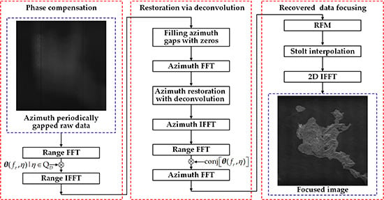
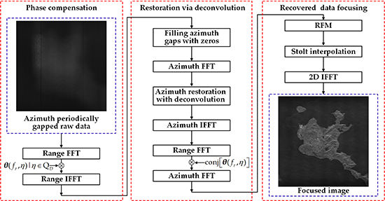
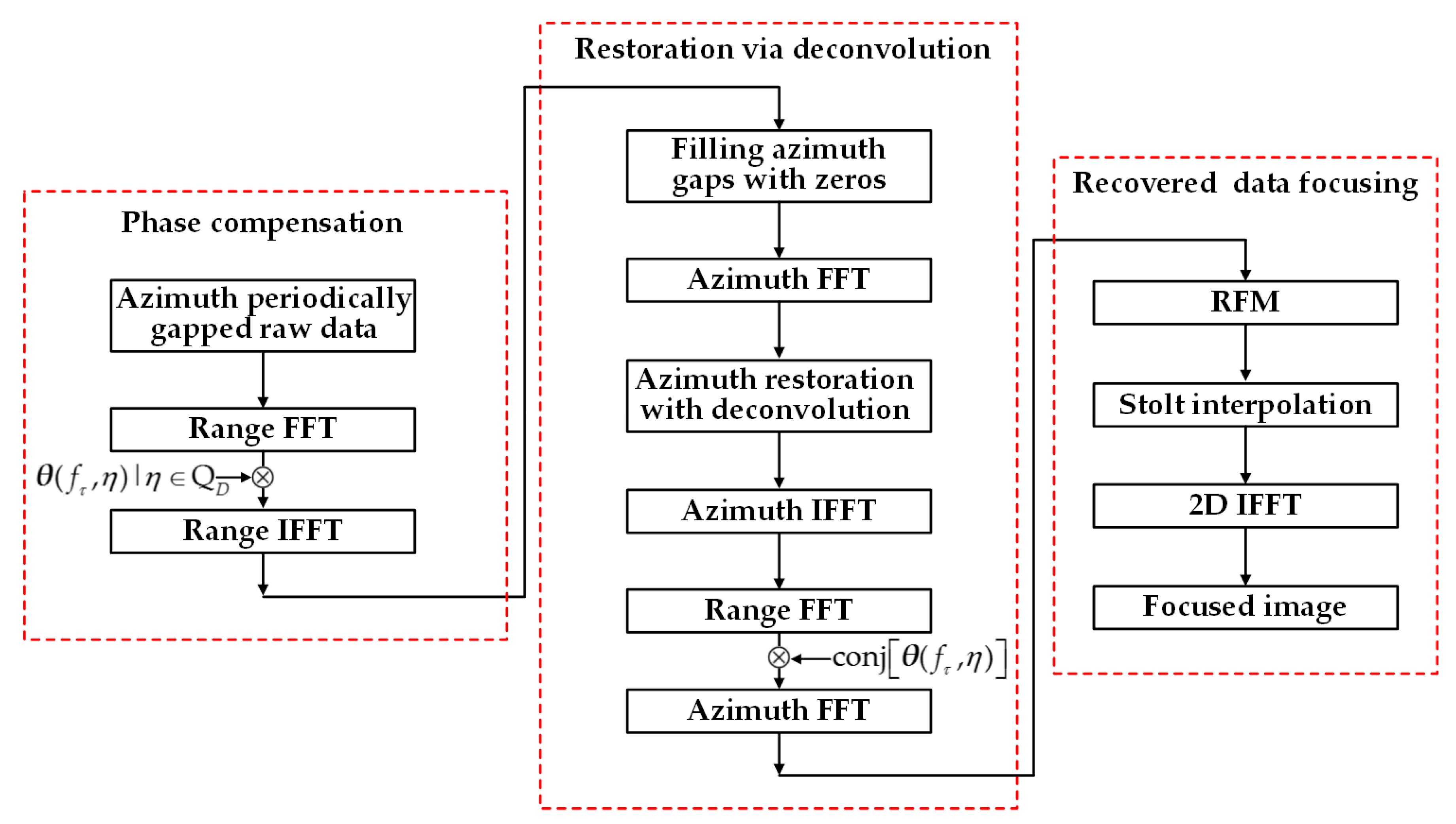
The proposed method for obtaining a focused image with deconvolution is described in this section. The phase compensation function, the restoration via deconvolution, a brief introduction of the RMA, and the procedure of the proposed method are presented.

2.1. Phase Compensation Function

Deconvolution can be regarded as a linear inverse problem. It is beneficial to solve linear inverse problems in a sparser domain [33]. In this case, it is significant to process the azimuth periodically gapped raw data in a sparser domain. In Section 2.1, a phase compensation function is designed to match the azimuth periodically gapped raw data in the range frequency domain. The phase compensation is implemented on raw data to remove modulation in the range direction and reduce most modulation in the azimuth direction. The data are compressed along the range direction in the range time domain due to the removal of range modulation. Moreover, the data are coarsely compressed along the azimuth direction in the azimuth frequency domain because of the reduction of the azimuth modulation. The azimuth frequency domain is also known as the Doppler domain. Therefore, the data are coarsely compressed in the range of the Doppler domain along both the range and azimuth direction after phase compensation. In other words, the energy of the data is more concentrated in the range of the Doppler domain after phase compensation. As a result, the gapped data become sparser in the range of the Doppler domain. Consequently, it is proper to restore the gapped data in the range of the Doppler domain after phase compensation. The description of the phase compensation function is derived and presented in this part.

In this paper, SAR is assumed to emit a pulse chirp signal and move with a uniform linear motion. After demodulation to its baseband, the echo data of a single point can be described by the range time τ and azimuth time η as below:

$$\begin{array}{ll}\mathit{s}(\tau ,\eta )=& {\mathit{w}}_{\mathit{r}}\left[\tau -\frac{2\mathit{R}(\eta )}{c}\right]{\mathit{w}}_{\mathit{a}}(\eta )\exp \left[\frac{-j4\pi f_0\mathit{R}(\eta )}{c}\right]\\ & \times \exp \left\{j\pi K_r{\left[\tau -\frac{2\mathit{R}(\eta )}{c}\right]}^2\right\},\eta \in Q_D\end{array}$$

(1)

In Equation (1), the amplitude factors are neglected. w_r is the range envelope, and w_a is the azimuth envelope. The velocity of light is denoted as c. The range frequency modulation rate is denoted as K_r. R(η) is the slant range between the target and radar at η, f₀ is the carrier frequency, and j is the imaginary unit. The complete SAR raw dataset is defined as a matrix with the size of N_r × N_a. The complete SAR raw data have N_r and N_a sampling points in the range and azimuth directions, respectively. Set D is defined as a set that includes indices of the available data in the azimuth periodically gapped raw data. The quantity of elements in set D is represented as N_D. In comparison with the complete SAR raw data, the set of available azimuth sampling time in the azimuth periodically gapped data is denoted as Q_D.

The slant range model can be regarded as a parabolic approximation of the Taylor expansion, as below:

$$\mathit{R}(\eta )=\sqrt{R_0^2+{\left(v\eta \right)}^2}\approx R_0+\frac{v^2{\eta }^2}{2R_0}$$

(2)

In Equation (2), v represents the velocity of the SAR platform, and R₀ represents the closest slant range. By operating Fourier transform (FT) along the range direction, the signal can be approximated as below:

$$\mathit{S}(f_{\tau },\eta )={\mathit{W}}_{\mathit{r}}(f_{\tau }){\mathit{w}}_{\mathit{a}}(\eta )\exp \left(-\frac{j\mathsf{\pi }{f}_{\tau }^2}{K_r}\right)\exp \left[-j4\mathsf{\pi }\frac{\left(f_0+f_{\tau }\right)\mathit{R}(\eta )}{c}\right]$$

(3)

Inspired by PFA [32], the phase compensation function is designed as below:

$$\mathit{\theta }(f_{\tau },\eta )=\exp \left(\frac{j\mathsf{\pi }{f}_{\tau }^2}{K_r}\right)\exp \left[\frac{j4\mathsf{\pi }\left(f_0+f_{\tau }\right){\mathit{R}}_{\mathit{ref}}(\eta )}{c}\right]$$

(4)

The reference slant range at the azimuth time is presented in the following formula:

$${\mathit{R}}_{\mathit{ref}}(\eta )=\sqrt{R_{0,ref}^2+{\left(v\eta \right)}^2}\approx R_{0,ref}+\frac{v^2{\eta }^2}{2R_{0,ref}}$$

(5)

In Equation (5), R_0,ref is the closest reference slant range. Afterwards, the signal after multiplication with the phase compensation function can be expressed as below:

$$\begin{array}{ll}{\mathit{S}}_{\mathit{c}}(f_{\tau },\eta )& =\mathit{S}(f_{\tau },\eta )\mathit{\theta }(f_{\tau },\eta )\\ & ={\mathit{W}}_{\mathit{r}}(f_{\tau }){\mathit{w}}_{\mathit{a}}(\eta )\exp \left\{\frac{-j4\mathsf{\pi }\left(f_0+f_{\tau }\right)\left[\mathit{R}(\eta )-{\mathit{R}}_{\mathit{ref}}(\eta )\right]}{c}\right\}\end{array}$$

(6)

By implementing inverse FT to S_c(τ,f_η) along the range direction, the result can be presented as below:

$${\mathit{s}}_{\mathit{c}}(\tau ,\eta )={\mathit{p}}_{\mathit{r}}\left\{\tau -\frac{2\left[\mathit{R}(\eta )-{\mathit{R}}_{\mathit{ref}}(\eta )\right]}{c}\right\}{\mathit{w}}_{\mathit{a}}(\eta )\exp \left\{-j4\mathsf{\pi }{f}_0\frac{\left[\mathit{R}(\eta )-{\mathit{R}}_{\mathit{ref}}(\eta )\right]}{c}\right\}$$

(7)

In Equation (7), p_r denotes the sinc function in the range direction. Substituting Equations (2) and (5) into Equation (7), s_c(τ,η) can be presented as follows:

$${\mathit{s}}_{\mathit{c}}(\tau ,\eta )=p_r\left\{\tau -\frac{2\left[\mathit{R}(\eta )-{\mathit{R}}_{\mathit{ref}}(\eta )\right]}{c}\right\}{\mathit{w}}_{\mathit{a}}(\eta )\exp \left\{-j4\mathsf{\pi }{f}_0\frac{\left(R_0-R_{0,ref}\right)}{c}\right\}\exp \left\{\frac{-j2\mathsf{\pi }{f}_0{v}^2}{c}\left(\frac{1}{R_0}-\frac{1}{R_{0,ref}}\right){\eta }^2\right\}$$

(8)

As illustrated in Equation (8), the second exponential term shows that the bandwidth of the azimuth modulation is almost removed after phase compensation in the range frequency. In addition, the signal has been compressed in the range direction, as the range modulation has been removed by phase compensation in the range frequency. Consequently, s_c(τ,η) is considered to be coarsely compressed in the range of the Doppler domain. In other words, the S_c(τ,f_η) is coarsely compressed.

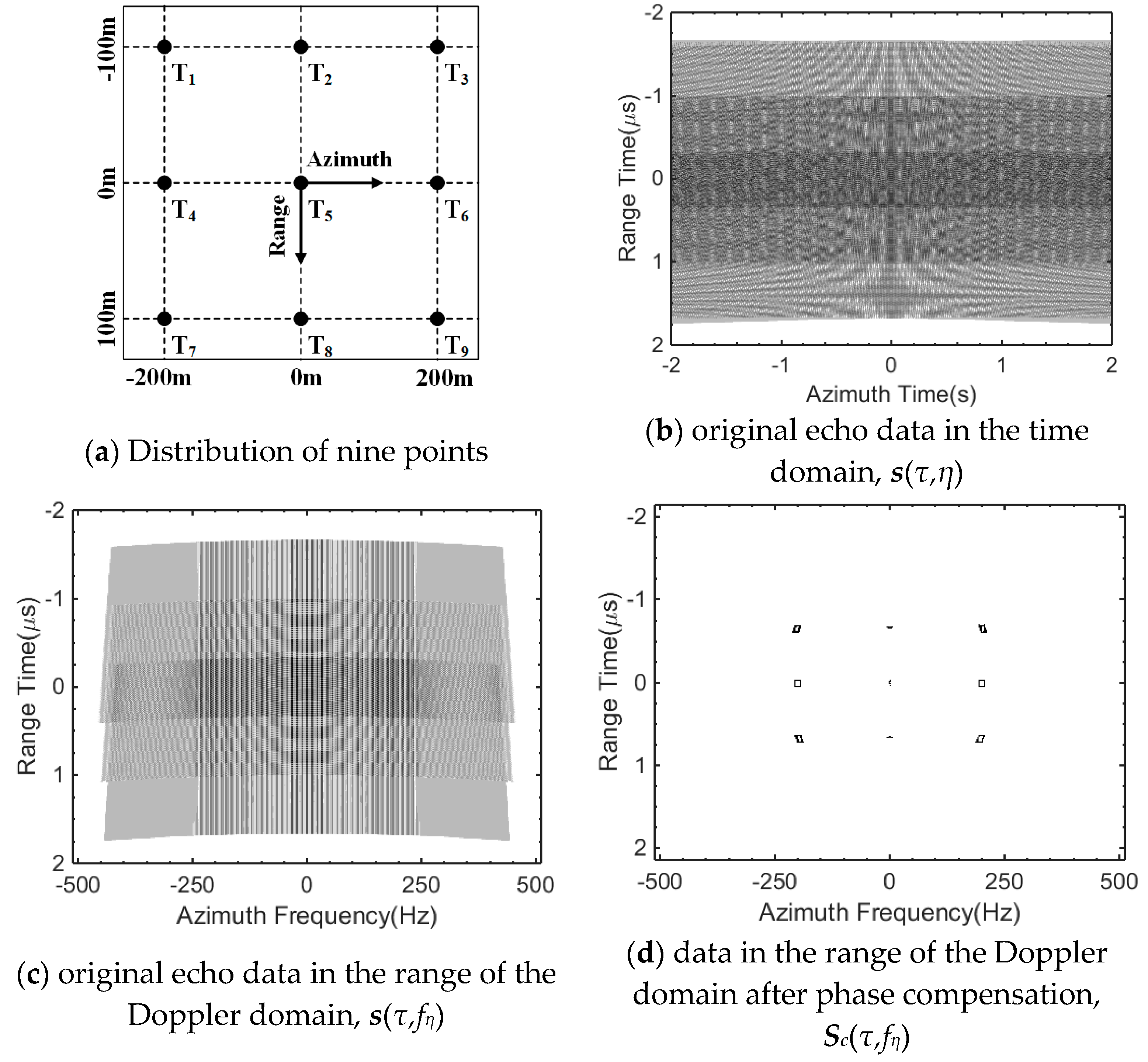
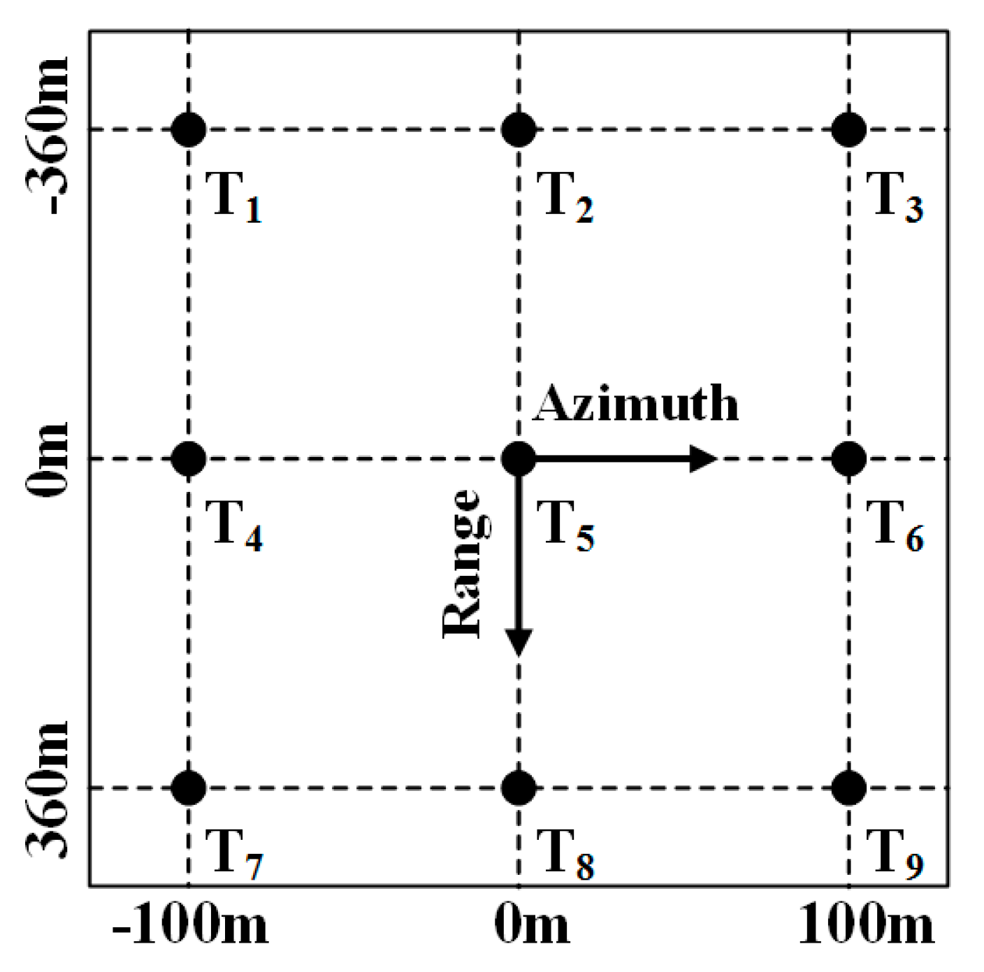
The coarse compression in the range of the Doppler domain after phase compensation is presented in Figure 3 and Figure 4. Figure 3 and Figure 4 demonstrate the coarse compression of point targets and real SAR data, respectively. In the depiction of the coarse compression of point targets, nine point targets are positioned to generate echo data. A distribution of the nine point targets is displayed in Figure 3a. The original echo data in the time domain are shown in Figure 3b. As shown in Figure 3b, the original echo data are dense in the time domain. Figure 3c,d illustrates the original echo data and the data with compensation in the range of the Doppler domain, respectively. Figure 3c shows that the original echo data are also dense in the range of the Doppler domain. Figure 3d indicates that the data become sparser around the Doppler domain after phase compensation in the range of the frequency domain. 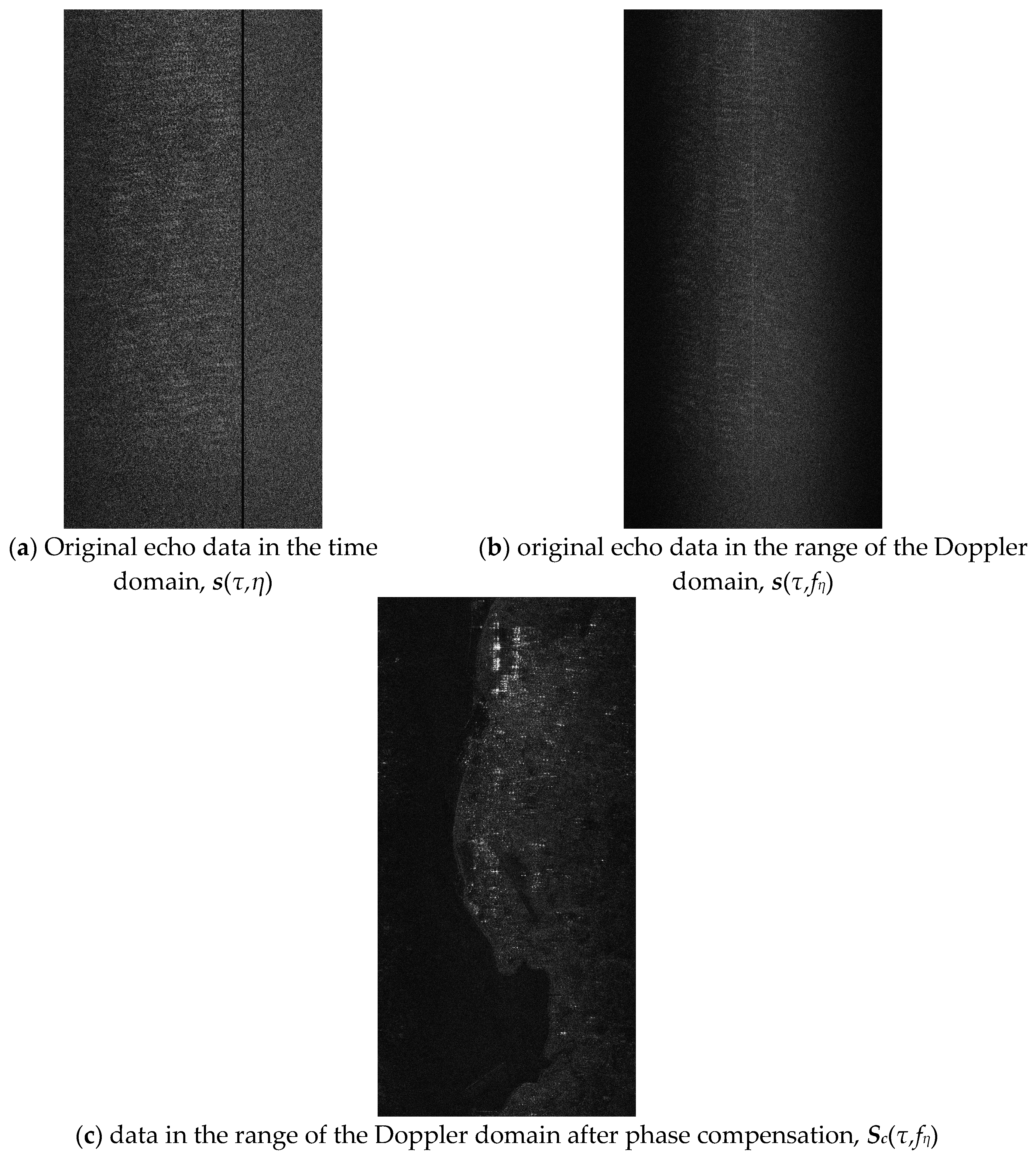Figure 4a shows the original echo data for real SAR data in the time domain, and Figure 4b demonstrates the original echo data for real SAR data in the range of the Doppler domain. Moreover, the real SAR data in the range of the Doppler domain after phase compensation is presented in Figure 4c. Figure 4c illustrates the real SAR data in coarse compression in the range of the Doppler domain after phase compensation. The s(τ,η) denotes the original echo data in the time domain. The s(τ,f_η) denotes the original echo data in the range of the Doppler domain. The S_c(τ,f_η) denotes the data in the range of the Doppler domain after phase compensation.

To further verify the coarse compression in the range of the Doppler domain after phase compensation, the analysis of coarse compression is listed in

Table 1. Analysis of coarse compression.

	IE		IC
	Point Target	Real SAR Data	Point Target	Real SAR Data
s(τ,η)	15.6475	13.9677	1.3344	1.1625
s(τ,fη)	15.3237	13.8575	1.8670	1.4381
Sc(τ,fη)	8.5858	13.1141	344.5768	11.6098

. Image contrast (IC) [35] and Image Entropy (IE) [36] are chosen as the criteria to assess the sparsity of the original echo data in the time domain, the original echo data in the range of the Doppler domain, and the data in the range of the Doppler domain after phase compensation. The IE and IC in Table 1 are all obtained with whole images in Figure 3b–d, Figure 4a–c. The more concentrated the energy of the SAR image is, the sparser the SAR image is. Moreover, if the energy of the SAR image is more concentrated, the IC of the SAR image has an increasing trend, and the IE of SAR image has a decreasing trend. As demonstrated in Table 1, the data in the range of the Doppler Domain after phase compensation have the largest IC and smallest IE for point targets and real SAR data, in contrast with the original echo data in the time domain and the range of the Doppler domain. As demonstrated in Table 1, the effect of concentrating the energy of data is more apparent in point scatters than in real SAR data. Similarly, the presented transformation for making data sparser also has a limited effect on surface scatters. Consequently, it can be concluded that the data in the range of the Doppler Domain after phase compensation are sparser than the original echo data in the time domain and the Doppler domain. In summary, the SAR data become much sparser around the Doppler domain after phase compensation in the range frequency domain.

Although the proposed phase compensation function is effective in the described scenario in Section 2.1, it also has limitations. The compensation occurs only for the reconstruction strategies because the interpolation error is data dependent. The proposed method performs satisfactorily over point scatters while the performance of the proposed method over surface scatters may decrease. If the platform of SAR has complicated motion rather than uniform linear motion, the approximation in Equation (5) may become invalid. A possible solution for the inaccuracy of Equation (5) is to develop a more accurate range model to accommodate for complicated motion. In addition, the proposed transformation does not consider high squint. Consequently, the proposed phase compensation requires extension in the scenario with high squint. Moreover, the proposed transformation may perform better in a wide-swath scenario with the implementation of a proper sub-block partition.

2.2. Restoration via Deconvolution

As presented in Section 2.1, the raw data become sparser in the range of the Doppler domain after phase compensation in the range of the frequency domain. Hence, it is feasible to recover the azimuth periodically gapped raw data in the Doppler domain after phase compensation. In this part, the description of restoring the azimuth periodically gapped raw data in the Doppler domain via complex deconvolution is presented.

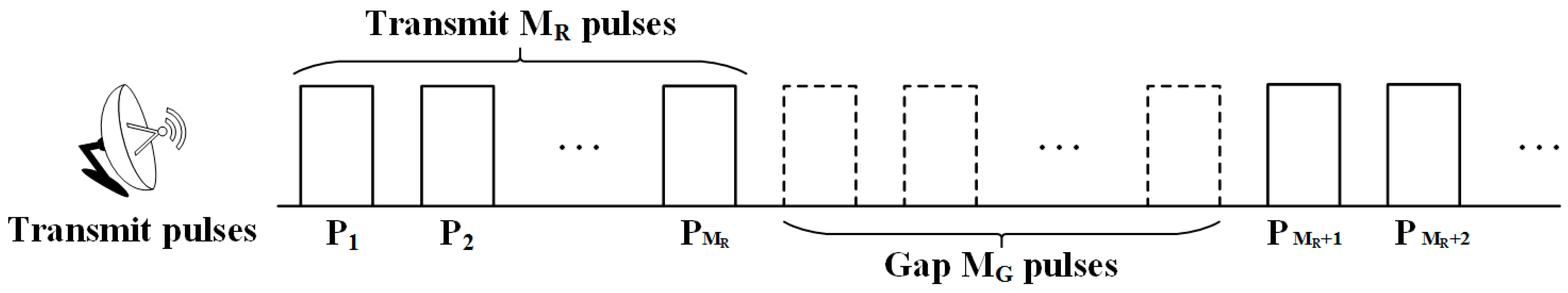
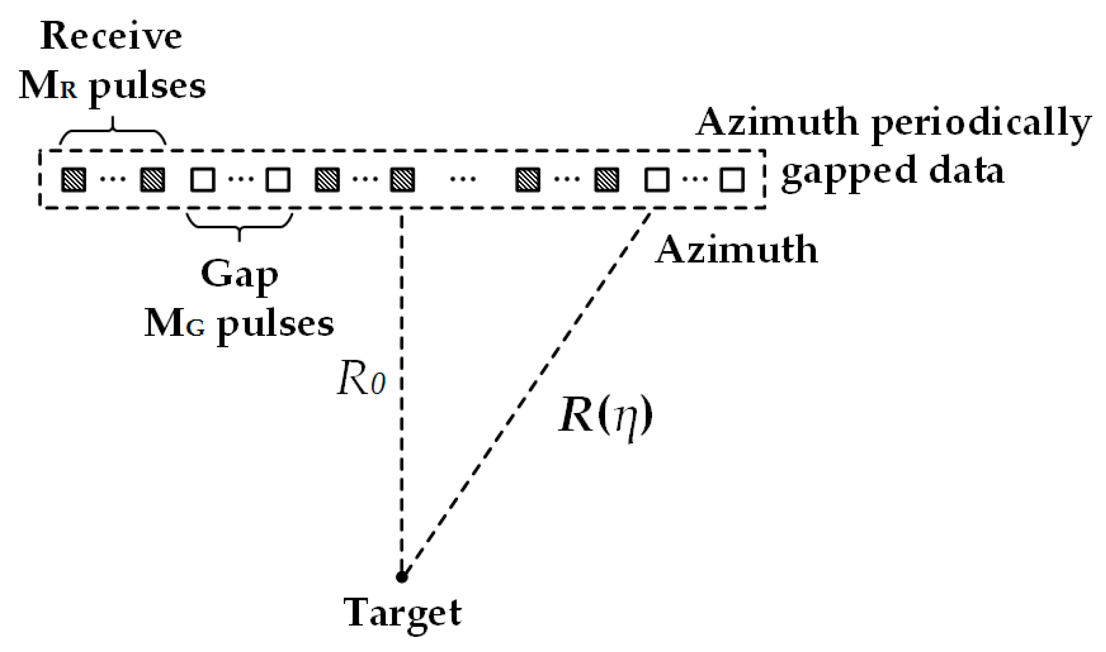
Figure 5 describes the sampling of SAR azimuth periodically gapped data. The shadow square represents the received pulse and the white square represents the gapped pulse. The complete dataset has N_a sampling pulses, while the gapped data have N_D sampling pulses in the azimuth direction. The azimuth periodically gapped data has N_C clusters of samples, and each cluster contains M_R available pulses and M_G gapped pulses. M_P denotes the periodicity of the gapping and equals the sum of M_R and M_G. Therefore, N_a=(M_R+M_G)N_C=M_PN_C and N_D=M_RN_C. In this paper, the proposed method is developed to cope with the SAR data, which is periodically gapped in the azimuth direction. As a result, the structure of the periodically gapped data is exploited to derive restoration with complex deconvolution in the following section.

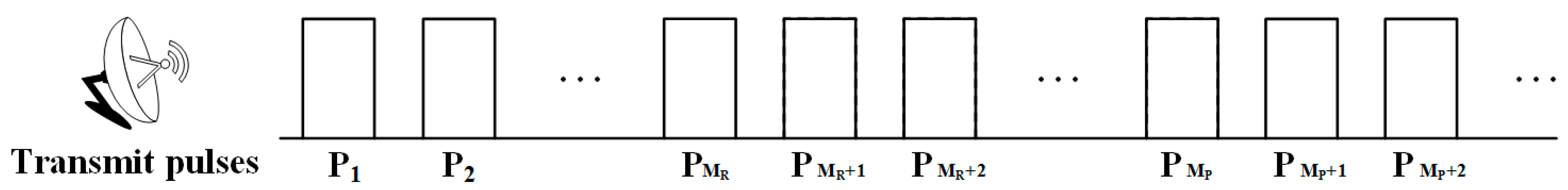
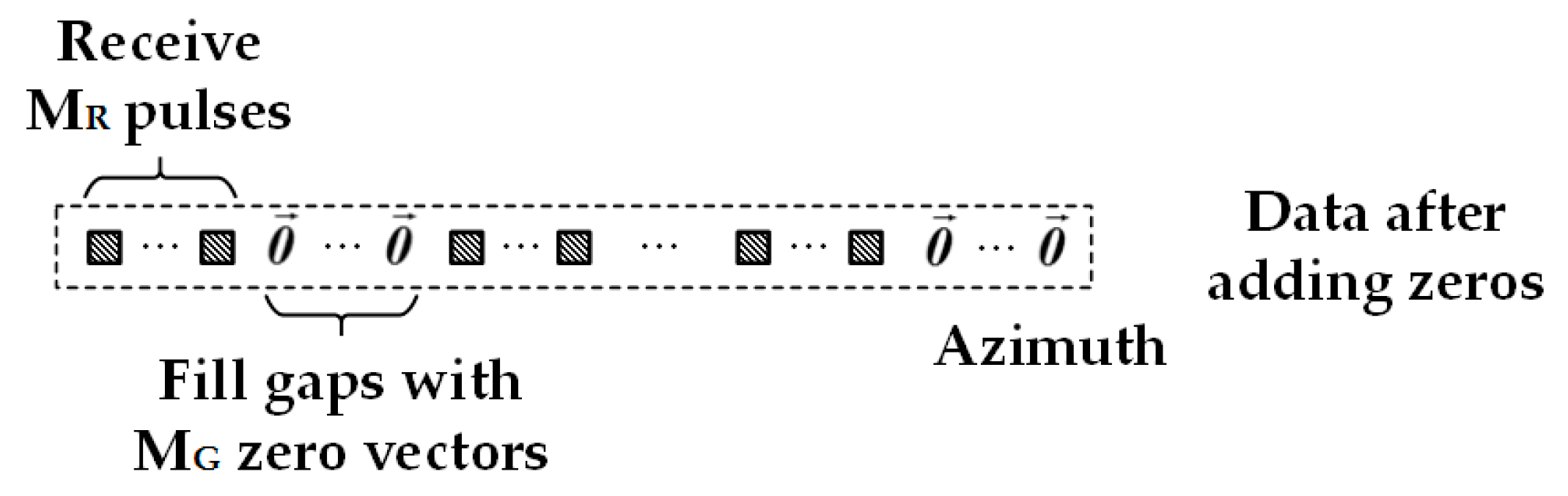
Figure 6 demonstrates filling gaps with zeros. As shown in Figure 6, the positions of gaps are filled with zero vectors. A zero vector has the same size as the pulse in the echo data. Therefore, the size of the data is N_r×N_a after the adding zeros operation.

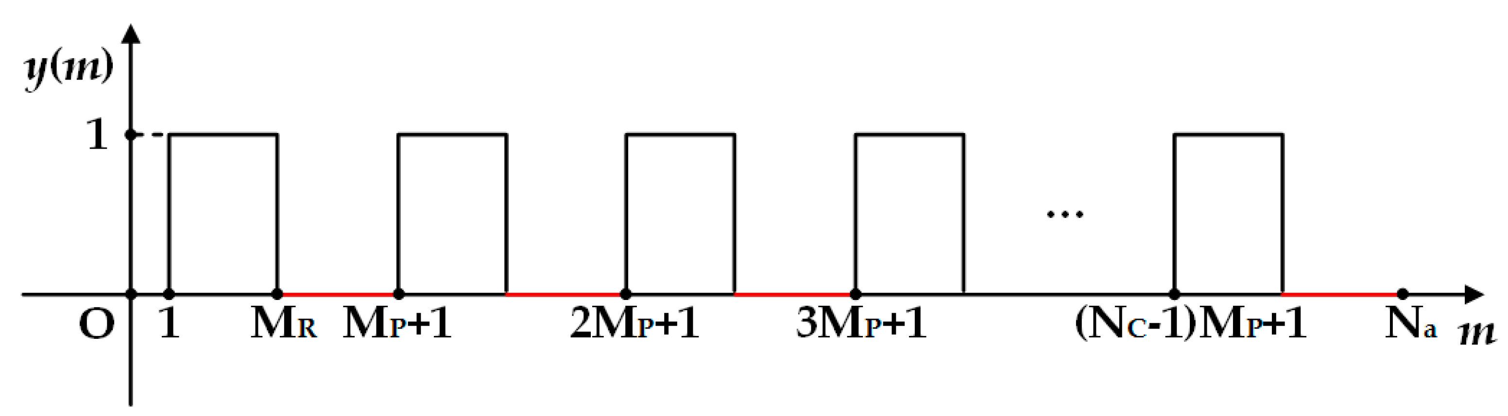
After zero padding in the gapped positions of the azimuth gapped data, the azimuth periodically gapped raw data can be treated as the multiplication between the complete raw data and the rectangular pulse sequence. The rectangular pulse sequence can be expressed as follows:

$$y(m)=\{\begin{array}{ll}1,\hfill & 1\le \mathrm{mod}(m,{\mathrm{M}}_{\mathrm{P}})\le {\mathrm{M}}_{\mathrm{R}}\\ 0,\hfill & {\mathrm{M}}_{\mathrm{R}}+1\le \mathrm{mod}(m,{\mathrm{M}}_{\mathrm{P}})\le {\mathrm{M}}_{\mathrm{P}}\end{array}m=1,2,3,\dots ,N_a$$

(9)

In Equation (9), the mod (m,M_P) denotes modulo operation, where m is the dividend and M_P is the divisor. The modulo operation returns the remainder after the division of m by M_P.

Figure 7 presents the demonstration of the rectangular pulse sequence. The rectangular pulse sequence is acquired according to Equation (9). In Figure 7, O denotes the origin of coordinates. The y(m) is plotted on the vertical axis against m on the horizontal axis in Figure 7. The black solid lines in Figure 7 represent elements that equal “1” in the rectangular pulse sequence, and the red solid lines in Figure 7 represents elements that equal “0” in the rectangular pulse sequence. The y(m) is an N_a×1 vector.

Azimuth periodically gapped raw data can be regarded as the multiplication between the complete raw data and rectangular pulse sequence in the azimuth time domain after zero padding. Hence, the azimuth spectrum of gapped data after zero padding can be represented as the convolution between the azimuth spectrum of complete data and the spectrum of the rectangular pulse sequence. Consequently, it is feasible to restore the azimuth spectrum of complete data by deconvoluting the azimuth spectrum of the azimuth periodically gapped data with the spectrum of the rectangular pulse sequence. In complex deconvolution, the spectrum of the rectangular pulse sequence acts as the point spread function. Therefore, it is necessary to derive the expression for the spectrum of the rectangular pulse sequence.

The expression for the spectrum of the rectangular pulse sequence in the discrete domain is derived with Equation (9) and the definition of Fast Fourier Transform (FFT), as follows:

$$\begin{array}{ll}\mathit{Y}(k)& ={\displaystyle \sum _{m=1}^{N_a}\mathit{y}(m)W_{N_a}^{(\mathrm{m}-1)(\mathrm{k}-1)}}\\ & =(W_{N_a}^{0\cdot (\mathrm{k}-1)}+W_{N_a}^{1\cdot (\mathrm{k}-1)}+W_{N_a}^{2\cdot (\mathrm{k}-1)}+\cdot \cdot \cdot +W_{N_a}^{({\mathrm{M}}_{\mathrm{R}}-1)\cdot (\mathrm{k}-1)})(1+\mathit{q}+{\mathit{q}}^2+\dots +{\mathit{q}}^{{\mathit{N}}_{\mathit{C}}-1})\\ & k=1,2,3,\dots ,N_a\end{array}$$

(10)

The definitions of W_Na and q are expressed in Equations (11) and (12), as follows:

$${\mathit{W}}_{N_a}={\mathbf{e}}^{-j\frac{2\pi }{N_a}}$$

(11)

$$\mathit{q}={\mathit{W}}_{N_a}^{M_P(k-1)}$$

(12)

As shown in Equation (10), the spectrum of the rectangular pulse sequence can be represented as the multiplication of two geometric sequences. According to the summation formula of the geometric sequence, the spectrum of the rectangular pulse sequence in the discrete domain can be expressed as follows:

$$\mathit{Y}(k)=\{\begin{array}{ll}{M}_R{N}_C\hfill & ,k=1\\ \frac{1-W_{N_a}^{{\mathrm{M}}_R(k-1)}}{1-W_{N_a}^{k-1}}·\frac{1-q^{N_C}}{1-q}\hfill & ,k=2,3,\dots ,N_a\end{array}$$

(13)

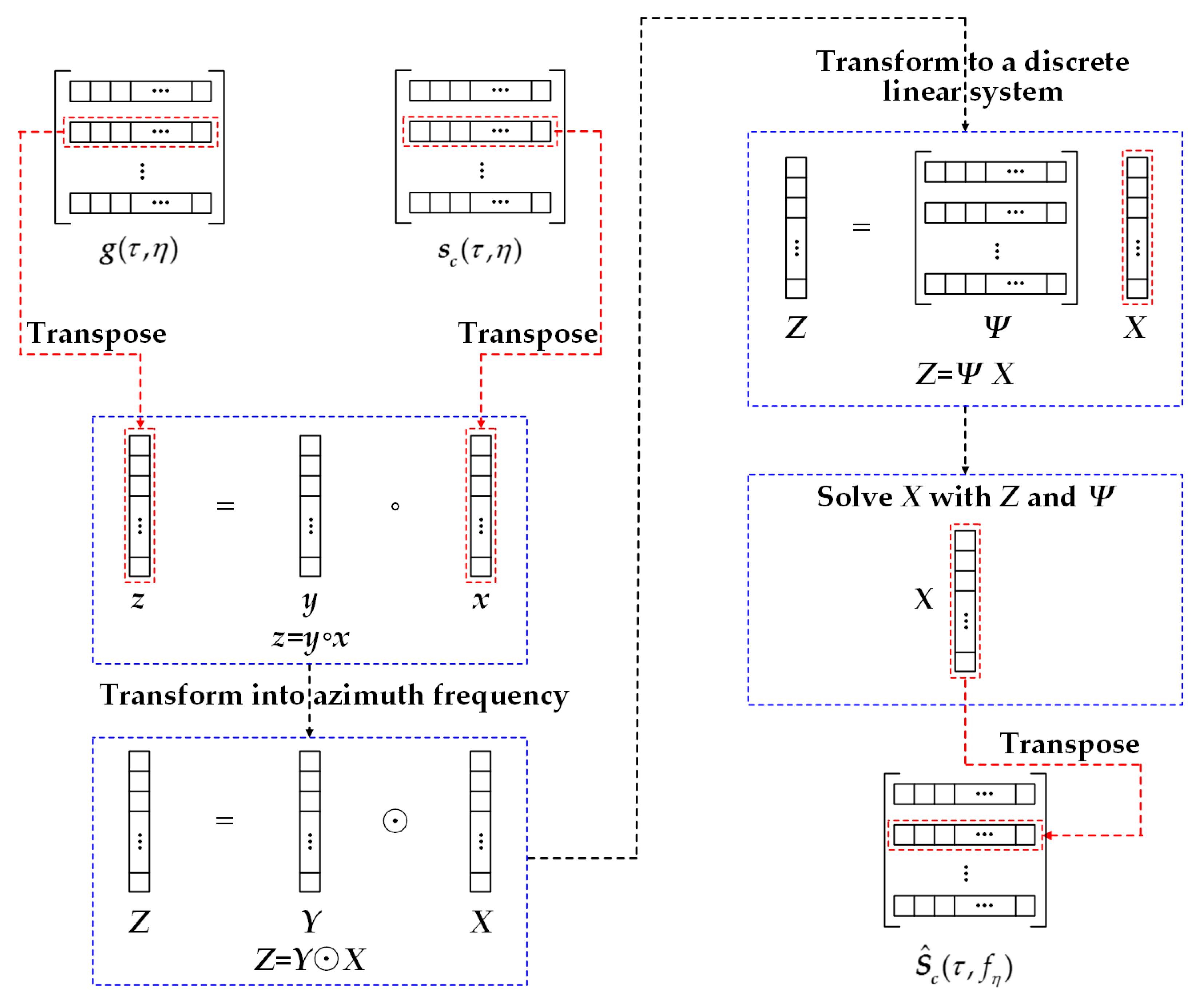
Figure 8 presents the procedure for restoration via complex deconvolution. The azimuth periodically gapped raw data are processed in the Doppler domain after phase compensation. The g(τ,η) denotes the azimuth periodically gapped data after phase compensation in the range frequency domain and a subsequent adding zeros operation in the time domain. The adding zeros operation fills the positions of gaps with zero vectors. The size of the g(τ,η) is N_r×N_a. The s_c(τ,η) denotes the complete echo data in the time domain after phase compensation in the range frequency domain. The size of s_c(τ,η) is N_r×N_a.

The N_a×1 vector x is defined as the transposed vector of any range time τ in the data s_c(τ,η). The N_a×1 vector z is defined as the transposed vector of any range time τ in the data g(τ,η). Thus, there exists a connection, as follows:

$$\mathit{z}=\mathit{y}\circ \mathit{x}$$

(14)

In Equation (14), the ◦ denotes the pointwise multiplication operation between two vectors. On the basis of the properties of Fourier transform, the relationship between the spectrums of x, y, and z can be expressed as follows:

$$\mathit{Z}=\mathit{Y}\odot \mathit{X}$$

(15)

In Equation (15), ⊙ denotes the circular convolution operation between two vectors. As the lengths of X, Y, and Z are all N_a, the convolution in Equation (15) is circular convolution rather than linear convolution.

This is the key point to solving the unknown X with the known Y and Z in Equation (15). To solve this deconvolution problem more conveniently, it is feasible to transform Equation (15) into another discrete linear system, as follows:

$$\mathit{Z}=\mathit{\Psi }\mathit{X}$$

(16)

In Equation (16), the matrix Ψ is the circular convolution operator. Multiplication between the matrix Ψ and the vector X equals the circular convolution between vector Y and vector X. The matrix Ψ is a circulant matrix, which is formed with vector Y according to the definition of circular convolution. The matrix Ψ can be expressed as follows:

$$\mathit{\Psi }=\left[\begin{array}{cccccc}\mathit{Y}({\mathrm{N}}_a)& \mathit{Y}({\mathrm{N}}_a-1)& \mathit{Y}({\mathrm{N}}_a-2)& \mathit{Y}({\mathrm{N}}_a-3)& \cdots & \mathit{Y}(1)\\ \mathit{Y}(1)& \mathit{Y}({\mathrm{N}}_a)& \mathit{Y}({\mathrm{N}}_a-1)& \mathit{Y}({\mathrm{N}}_a-2)& \cdots & \mathit{Y}(2)\\ \mathit{Y}(2)& \mathit{Y}(1)& \mathit{Y}({\mathrm{N}}_a)& \mathit{Y}({\mathrm{N}}_a-1)& \cdots & \mathit{Y}(3)\\ ⋮& ⋮& ⋮& ⋮& \ddots & ⋮\\ \mathit{Y}({\mathrm{N}}_a-2)& \mathit{Y}({\mathrm{N}}_a-3)& \mathit{Y}({\mathrm{N}}_a-4)& \mathit{Y}({\mathrm{N}}_a-5)& \cdots & \mathit{Y}({\mathrm{N}}_a-1)\\ \mathit{Y}({\mathrm{N}}_a-1)& \mathit{Y}({\mathrm{N}}_a-2)& \mathit{Y}({\mathrm{N}}_a-3)& \mathit{Y}({\mathrm{N}}_a-4)& \cdots & \mathit{Y}({\mathrm{N}}_a)\end{array}\right]$$

(17)

As shown in Equation (17), the matrix Ψ has a form where each row is a cyclic shift of the row above it. The size of the matrix Ψ is N_a×N_a.

Consequently, the deconvolution problem is transformed by estimating the unknown X from the known Z and Ψ. This problem can be cast as a linear inverse problem, and the ISTA is capable of dealing with this problem. The ISTA (Iterative Shrinkage-Thresholding Algorithm) [33] solves the linear inverse problem via the method of l₁ regularization. The deconvolution belongs to an ill-conditioned problem and has a very large norm. In this case, regularization is utilized to replace the large norm by approximants with a smaller norm, so numerically stable solutions can be defined and used as meaningful approximations of the true solution corresponding to the exact data [33]. The l₁ regularization seeks to find the solution of

$$\underset{\mathit{X}}{\min }\left\{\mathit{F}(\mathit{X})\equiv {\Vert \mathit{\Psi }\mathit{X}-\mathit{Z}\Vert }^2+\mathit{\beta }{\Vert \mathit{X}\Vert }_1\right\}$$

(18)

In Equation (18), the ║•║₁ stands for the sum of the absolute values of the components of X. The general step of ISTA is

$${\mathit{X}}^{p+1}={\mathit{\Gamma }}_{\beta t}\left[{\mathit{X}}^p-2t{\mathit{\Psi }}^T\left(\mathit{\Psi }{\mathit{X}}^p-Z\right)\right]$$

(19)

In Equation (19), t is the proper stepsize, p denotes the iteration number, and Γ_α is the shrinkage operator defined as

$${\mathit{\Gamma }}_{\beta t}(\mathit{B})=\max \left(\left|\mathit{B}\right|-\beta t,0\right)\mathrm{sgn}(\mathit{B})$$

(20)

In Equation (20), the max(∙) denotes finding the maximum value operation and the sgn(∙) denotes the sign function. As the sign function is included in Equation (20), the shrinkage operator in Equation (20) can only be implemented in the field of real numbers. However, SAR data are complex data. To process complex data, the shrinkage operator needs modification. The modified shrinkage operator for dealing with complex data is given in [37], as follows:

$${\mathit{\Gamma }}_{\beta t}(\mathit{B})=\max \left(\left|\mathit{B}\right|-\beta t,0\right)\frac{\mathit{B}}{\left|\mathit{B}\right|}$$

(21)

With the implementation of ISTA via Equations (19) and (21), X can be restored from the known Y and Z via complex deconvolution. Consequently, the azimuth spectrum of complete data can be recovered by deconvoluting the azimuth spectrum of the azimuth periodically gapped data with the spectrum of the rectangular pulse sequence in the range of the Doppler domain. The estimation of S_c(τ,f_η) is denoted as ${\hat{\mathit{S}}}_c(\tau ,f_{\eta })$, which is restored from g(τ,f_η) and Y via the operation of deconvolution. Then, the recovery of the two-dimensional (2D) spectrum of the raw data can be acquired as follows:

$${\hat{\mathit{S}}}_{2\mathrm{df}}(f_{\tau },f_{\eta })=\mathrm{FTa}\left\{\mathrm{FTr}\left\{\mathrm{IFTa}\left[{\hat{\mathit{S}}}_{\mathit{c}}(\tau ,f_{\eta })\right]\right\}·\mathrm{conj}\left[\mathit{\theta }(f_{\tau },\eta )\right]\right\}$$

(22)

The IFTa[∙] denotes inverse Fourier Transform (FT) along azimuth direction. FTa[∙] denotes the FT along the azimuth direction. FTr[∙] denotes the FT along the range direction and conj[∙] represents the conjugate operation. After the raw data have been recovered, traditional SAR imaging algorithms are capable of focusing the recovered SAR raw data.

2.3. Range Migration Algorithm

A brief introduction on the Range Migration Algorithm (RMA) is presented in this section. The RMA is proposed with the condition of uniform linear motion. By operating two-dimensional (2D) FT on Equation (1) along with the range model in Equation (2), the expression of the 2D spectrum of the echo signal can be given as follows:

$${\mathit{S}}_{2\mathit{d}\mathit{f}}(f_{\tau },f_{\eta };\mathrm{T})={\mathit{W}}_{\mathit{r}}(f_{\tau }){\mathit{W}}_{\mathit{a}}(f_{\eta })\exp \left[-j\frac{4\pi r}{c}\sqrt{{\left(f_0+f_{\tau }\right)}^2-\frac{c^2{f}_{\eta }^2}{4v^2}}-j\pi \frac{f_{\tau }^2}{K_r}\right]$$

(23)

In Equation (23), f_τ and f_η are the range frequency and azimuth frequency. In addition, W_r(•) is the envelope of the range frequency and W_a(•) is the envelope of the azimuth frequency.

The first key step in RMA is the Reference Function Multiplication (RFM). The reference function in the 2D frequency domain can be selected as conj[S_2df(f_τ,f_η;T_ref)], which is the conjugated 2D spectrum of the reference target. T_ref represents the reference point target, and conj[•] represents the conjugation operation.

The step of the RFM operation can be given as follows:

$$\begin{array}{ll}{\mathit{S}}_{\mathit{R}\mathit{F}\mathit{M}}(f_{\tau },f_{\eta };\mathrm{T})& =S_{2\mathit{d}\mathit{f}}(f_{\tau },f_{\eta };\mathrm{T})\mathrm{conj}\left[{\mathit{S}}_{2\mathit{d}\mathit{f}}(f_{\tau },f_{\eta };{\mathrm{T}}_{\mathrm{ref}})\right]\\ & ={\mathit{W}}_r(f_{\tau }){\mathit{W}}_{\mathit{a}}(f_{\eta })\exp \left[-j\frac{4\pi (r-r_{ref})}{c}\sqrt{{\left(f_0+f_{\tau }\right)}^2-\frac{c^2{f}_{\eta }^2}{4v^2}}\right]\end{array}$$

(24)

The RFM operation totally removes the range migration of every target in the reference range. However, the RFM only partly removes the range migration of each target in other ranges. Hence, a subsequent Stolt interpolation is used to cancel the residual quadratic and higher order phase modulation. In uniform linear motion, the Stolt interpolation is presented as follows:

$$\sqrt{{\left(f_0+f_{\tau }\right)}^2-\frac{c^2{f}_{\eta }^2}{4v^2}}=f_0+f_{\tau }^{\prime }$$

(25)

By performing the Stolt interpolation, the SAR data are transformed into a new 2D frequency domain (f_τ́, f_η), as follows:

$$\begin{array}{l}{\mathbf{S}}_{\mathit{R}\mathit{F}\mathit{M}}^{\prime }(f_{\tau }^{\prime },f_{\eta };\mathrm{T})\\ ={\mathit{W}}_{\mathit{r}}(f_{\tau }^{\prime }){\mathit{W}}_{\mathit{a}}(f_{\eta })\exp \left[-j\frac{4\pi (r-r_{ref})}{c}(f_0+f_{\tau }^{\prime })\right]\end{array}$$

(26)

By operating the 2D Inverse FT according to Equation (26), the echo data can be transformed into the time domain. Consequently, a well-focused SAR image is obtained as follows:

$${\mathit{I}}_{\mathit{RFM}}^{\prime }(\tau ,\eta ;\mathrm{T})=\sin \mathrm{c}\left[\tau -\frac{2(r-r_{ref})}{c}\right]\sin \mathrm{c}(\eta )$$

(27)

2.4. Procedure of Proposed Method

Figure 9 illustrates the flowchart of the proposed method. In the flowchart, IFFT denotes inverse FFT. The proposed method is generally comprised of three parts: phase compensation, restoration via complex deconvolution, and recovered data focusing. In phase compensation, the azimuth periodically gapped raw data are multiplied with θ(f_τ,η)|η∈Q_D in the range frequency domain. Θ(f_τ,η)|η∈Q_D is the phase compensation function for the azimuth periodically gapped data. After phase compensation in the range frequency domain, the gapped data are transformed back to the time domain and become sparser in the Doppler domain. The restoration via deconvolution starts with filling the azimuth gaps with zeros. Then, the estimation of S_c(τ,f_η) is recovered with g(τ,f_η) and Y via the operation of complex deconvolution. Complex deconvolution is implemented by seeking the solution for Equation (18). After estimating S_c(τ,f_η), the recovery of the 2D spectrum of the raw data can be obtained with Equation (22). As the 2D spectrum of raw data is recovered, the focused image can be acquired via recovered data focusing. The RMA is selected to focus the recovered data. The RFM and a subsequent Stolt interpolation are implemented to the recovered 2D spectrum of raw data. RFM and Stolt interpolation are two key steps in RMA. Afterwards, the focused image can be obtained by transforming the data into the time domain by 2D IFFT. The computational complexity of phase compensation is O(2N_DN_rlog₂(N_r)+ N_DN_r). The computation complexity of restoration via deconvolution is O((N_a-N_D)N_r +3N_aN_rlog₂(N_a)+5PN_aN_r+ N_aN_rlog₂(N_r)+ N_aN_r). The computation complexity of recovered data focusing is O(N_aN_r +N_aN_rlog₂(N_a)+ N_aN_rlog₂(N_r)+ 8N_aN_r).

3. Experimental Results

Experiments were implemented to assess the effectiveness of the proposed method. Firstly, the point target simulation was undertaken to demonstrate the validity of the proposed method. Then, the effectiveness of the proposed method was further validated with surface target simulation. Finally, real SAR data were utilized to demonstrate the performance of the proposed method.

3.1. Point Target Simulation

To appraise the performance of the proposed method, point target simulation was employed. Point target simulation was implemented under the condition of monostatic SAR by emitting a pulse linear frequency modulation signal. The system parameters for simulation are given in

Table 2. System parameters for point target simulation.

Parameter Name	Value	Units
Slant range of scene center	8	km
Transmitted pulse duration	2	μs
Signal bandwidth	300	MHz
Range sampling rate	360	MHz
Pulse repetition frequency	1536	Hz
Radar center frequency	10	GHz
Radar velocity	120	m/s
Range resolution	0.5	m
Azimuth resolution	0.5	m

. In point target simulation, the resolution was expected to achieve 0.5 m in the range direction and the azimuth direction. The mode of SAR operation was chosen as the spotlight SAR in point target simulation due to the demand of resolution.

Figure 10 displays the distribution of point targets in simulation. Nine point targets were positioned for point target simulation; these targets were labeled from T₁ to T₉. The size of the complete SAR raw data in the point target simulation was 5120×3072. The complete data had 5120 and 3072 sampling points in the range and azimuth direction.

The azimuth periodically gapped SAR raw data for simulation was obtained by generating a new matrix with extracting columns from complete SAR raw data periodically. In simulation, the gapped SAR data were generated via gapping every 16 pulses, and the size of the gapped data was 5120×1536. The parameter M_R was selected to be 16, and the parameter M_G was chosen to be 16 in the point target simulation. The gapping rate for point target simulation was 50% in the azimuth direction. In the point target simulation, the parameter β was set as 0.25, and the iteration number was set as 1000. Stepsize t was set as the maximum singular value of the matrix Ψ.

The focused results of the point target simulation are illustrated from Figure 11, Figure 12 and Figure 13. The focused results of the placed nine point targets are depicted in Figure 11a, Figure 12c and Figure 13c. In Figure 11, Figure 12 and Figure 13, the contour plots of the interpolated impulse response functions of the focused nine point targets are illustrated. The contour lines of -3 dB, -13 dB, -20 dB, and -30 dB were chosen to present the focused point targets. As displayed in Figure 11, Figure 12 and Figure 13, all nine point targets were focused satisfactorily.

Figure 14, Figure 15 and Figure 16 demonstrate the one-dimensional (1D) azimuth profiles of the imaged nine point targets via the adding zeros operation and the proposed method. The adding zeros operation entailed filling the gapping positions in the azimuth direction with zeros and the subsequent implementation of RMA. The existence of fake targets in the azimuth direction was the main problem in focusing azimuth periodically gapped data, which was caused by periodical azimuth gapping. As shown in Figure 14, Figure 15 and Figure 16, the fake targets were obviously suppressed via the implementation of the proposed method. Consequently, it can be concluded that the proposed method performed well in point target simulations. To assess the validity of the proposed method for point target simulation, the analysis of point target simulation is listed in Section 4.

3.2. Surface Target Simulation

The surface target simulation is presented in this part that verified the effectiveness of the proposed method. Many point targets were placed to form a surface target with the shape of capital letter “T”. The surface target simulation was carried out with the system parameters in

Table 3. System parameters for surface target simulation.

Parameter Name	Value	Units
Slant range of scene center	8	km
Transmitted pulse duration	2	μs
Signal bandwidth	600	MHz
Range sampling rate	720	MHz
Pulse repetition frequency	1024	Hz
Radar center frequency	10	GHz
Radar velocity	120	m/s
Range resolution	0.25	m
Azimuth resolution	0.25	m

. The complete raw SAR data in surface target simulation were a 3256×4096 matrix, which had range sampling points and azimuth sampling pulses. In surface target simulation, the gapped SAR data were generated by gapping every 16 pulses, and the size of the gapped data was 3256×2048. The parameter M_R was chosen to be 16, and the parameter M_G was selected to be 16 in the surface target simulation. The loss rate in surface target simulation was 50% in the azimuth direction. In the surface target simulation, the parameter β was set as 0.25, and the iteration number was set as 1000. Stepsize t was selected as the maximum singular value of the matrix Ψ.

Figure 17 demonstrates the results of surface target simulation with the adding zeros operation and the proposed method. Figure 18, Figure 19 and Figure 20 illustrate the 1D azimuth profiles of results in surface target simulation via the adding zeros operation and the proposed method. The 1D azimuth profiles in Figure 18, Figure 19 and Figure 20 are selected at -150 m, 0 m and 150 m in range direction, respectively. As shown in Figure 17a, many fake targets exist in the result obtained by the adding zeros operation. In contrast, Figure 17b demonstrates that fake targets were obviously suppressed with the implementation of the proposed method. Furthermore, the 1D azimuth profiles in Figure 18, Figure 19 and Figure 20 present more detailed comparison between results obtained by the adding zeros operation and the proposed method.

3.3. Real SAR Data Processing

Real SAR data were utilized to demonstrate the validity of the proposed method. The real SAR data for this experiment were collected by Sentinel-1A. The size of the complete real SAR data was 8192×8192. In other words, the complete real SAR data had 8192 sampling points in the range direction and 8192 sampling pulses in the azimuth direction.

The azimuth periodically gapped SAR raw data for the real SAR data processing were acquired by constructing a new matrix via extracting columns from complete real SAR data. In real SAR data processing, the gapped SAR data were obtained by gapping every 16 pulses, and the size of the gapped data was 8192×4096. The parameter M_R was chosen to be 16, and the parameter M_G was supposed to be 16 in real SAR data processing. The gapping rate for real data processing was 50% in the azimuth direction. In real SAR data processing, the parameter β was set as 0.25, and the iteration number was set as 800. The stepsize t was set as the maximum singular value of the matrix Ψ.

Figure 21 depicts the results of real SAR data processing. Figure 21a shows the imaging result obtained from the complete raw data via RMA. Figure 21b demonstrates the imaging result acquired via the adding zeros operation from the gapped data. The result in Figure 21b was acquired via filling the gapping positions in the azimuth direction with zeros and the subsequent implementation of RMA. Figure 21c illustrates the imaging result acquired with PG-APES. The PG-APES used to obtain Figure 21c was implemented by recovering the gapped data via PG-APES in the range of the Doppler domain and the subsequent operation of the RMA. Figure 21d is the imaging result acquired with the Burg algorithm. The image result in Figure 21d was obtained by recovering the gapped data via the method in [15] and a subsequent implementation of RMA. Figure 21e displays the imaging result acquired with the method in reference [23]. Figure 21f shows the imaging result acquired with the proposed method. In real SAR data images, the range and azimuth directions were the vertical and horizontal directions, respectively.

As demonstrated in Figure 21b, the phenomenon of ghost targets exists in the azimuth direction due to azimuth periodical gapping. With the application of different methods, the phenomenon of ghost targets was suppressed in different degrees via the demonstration in Figure 21c–f. Figure 21c,d,f indicates that the proposed method performed better than the PG-APES and Burg algorithm in suppressing ghost targets in the azimuth direction. Moreover, Figure 17e illustrates that the method in [23] performed competently in suppressing ghost targets. However, as shown in Figure 17e, unexpected fake strong scatters were induced by the method in [23] when M_R and M_G were both set as 16. Consequently, it can be concluded that the proposed method performed better than the other four methods in suppressing ghost targets. The validity of the proposed method for real SAR data is demonstrated in Figure 21f.

To demonstrate the validity of the proposed method further, three local regions were chosen to show more details. The three chosen regions are displayed in Figure 22 and are identified with red boxes. The results of the enlarged local regions of real SAR data are demonstrated in Figure 23, Figure 24 and Figure 25. The displayed enlarged local regions were acquired in six different ways. These six methods are as follows: obtaining the image from complete data via RMA, obtaining the image from the gapped data by adding zeros, obtaining the image from gapped data via PG-APES, obtaining the image from gapped data via the Burg algorithm, obtaining the image from the gapped data via the method in [23], and obtaining the image from the gapped data via the proposed method. The validity of the proposed method is verified further by Figure 23, Figure 24 and Figure 25.

4. Discussion

The focused results in Section 3 demonstrate the effectiveness of the proposed method. To evaluate the validity of the proposed method further, several criteria were selected to analyze the results of point target simulation and real SAR data processing.

To evaluate the performance of the proposed method on point target simulation, the impulse response width (IRW), peak sidelobe ratio (PSLR), and integrated sidelobe ratio (ISLR) were chosen as criteria for assessing the quality of focused point targets. To ensure the quality of focused point targets, the PSLR and ISLR are supposed to be less than -13 dB and -10.15 dB, respectively. In addition, because IRW is regarded as the image resolution in the scenario of SAR image, the IRW should not be inferior to 0.5 m when the resolution is expected to attain 0.5 m. In this paper, the main lobe width in ISLR is set to two times the IRW.

The analysis of the focused results in the point target simulation is illustrated in

Table 4. Analysis of point target simulation with the proposed method.

T	Range			Azimuth
	IRW (m)	PSLR (dB)	ISLR (dB)	IRW (m)	PSLR (dB)	ISLR (dB)
1	0.4458	-13.52	-10.89	0.4275	-13.18	-10.61
2	0.4417	-13.42	-10.87	0.4250	-13.23	-10.63
3	0.4455	-13.51	-10.88	0.4263	-13.25	-10.60
4	0.4479	-13.35	-10.57	0.4487	-13.37	-10.88
5	0.4458	-13.22	-10.34	0.4438	-13.12	-10.56
6	0.4460	-13.35	-10.56	0.4500	-13.34	-10.87
7	0.4462	-13.54	-11.08	0.4663	-13.20	-10.62
8	0.4396	-13.38	-10.08	0.4630	-13.06	-10.49
9	0.4462	-13.48	-11.05	0.4665	-13.09	-10.61

. As demonstrated in Table 4, all the focused point targets achieved the requirements of IRW, PSLR, and ISLR in both the range and azimuth direction.

Table 5. Analysis of fake targets in the point target simulation.

Row	Method
	Adding Zeros Operation	The Proposed Method
1	-12.63 dB	-49.16 dB
2	-12.54 dB	-51.36 dB
3	-11.03 dB	-35.75 dB

demonstrates the analysis of fake targets in point target simulation. Row 1 contains 1D azimuth profiles of T₁, T₂, and T₃. Row 2 contains 1D azimuth profiles of T₄, T₅, and T₆. Row 3 contains 1D azimuth profiles of T₇, T₈, and T₉. The amplitude of the highest fake target in each row is listed in Table 5. As shown in Table 4, fake targets were obviously suppressed with the implementation of the proposed method. Therefore, it can be concluded that the proposed method performed satisfactorily in point target simulation.

The analysis of fake targets in the surface target simulation is demonstrated in the

Table 6. Analysis of fake targets in the surface target simulation.

Row	Method
	Adding Zeros Operation	The Proposed Method
1	-5.18 dB	-10.76 dB
2	-16.63 dB	-27.21 dB
3	-16.83 dB	-26.31 dB

. In Table 5, Rows 1–3 represent 1D azimuth profiles at -150 m, 0 m and 150 m in the range direction, respectively. As illustrated in Table 6, fake targets were apparently suppressed with the operation of the proposed method. Comparing with the point target simulation, the performance of suppression on fake targets decreased in the surface target simulation.

To analyze the results of real SAR data processing, IE and IC were utilized to assess the imaging quality of real SAR data results. In addition, the MSE (Mean Square Error) was also utilized to analyze the results of real SAR data processing. The focused result of complete real SAR data was defined as the ground truth image in this study. The MSE analysis of real SAR data processing was obtained with respect to the ground truth image. IE and IC analyses of the real SAR data results are given in

Table 7. IE and IC analysis for the results of real SAR data processing.

	IE				IC
	Whole	Region 1	Region 2	Region 3	Whole	Region 1	Region 2	Region 3
Complete data	17.02	13.68	14.38	14.30	7.99	12.71	2.54	2.68
Adding zeros	17.15	14.00	14.53	14.44	4.72	7.36	1.74	1.94
PG-APES	17.22	14.25	14.57	14.49	3.55	5.85	1.53	1.67
Burg	17.05	13.79	14.47	14.37	5.89	9.07	1.92	2.10
Method in [23]	16.98	13.65	14.24	14.28	7.60	12.55	2.64	2.67
Proposed method	17.04	13.72	14.41	14.39	9.13	14.29	2.69	2.61

. The results of the whole scene and local regions are analyzed in Table 7. Generally, better focusing leads to a larger IC and smaller IE [35,36]. As displayed in Table 7, the proposed method generally performed better than the adding zeros operation, PG-APES, and Burg algorithm with the IE and IC criteria. Because of the existence of some fake strong scattering points, the method in [23] had a larger IC in Region 3 than the proposed method, and the method in [23] had a smaller IE than the proposed method. The differences among the results acquired via the adding zeros operation, PG-APES, Burg algorithm, the method in [23], and the proposed method were not apparent in the IE criterion. The IE and IC analyses of real SAR data processing were generally consistent with the results shown in Figure 21 and Figure 23, Figure 24 and Figure 25. The MSE analysis for the results of real SAR data processing is presented in

Table 8. MSE analysis for the results of real SAR data processing.

	MSE
	Whole	Region 1	Region 2	Region 3
Adding zeros	1.7382	6.5166	28.2920	15.7520
PG-APES	2.7807	5.1541	15.0794	10.9907
Burg	2.1794	5.4941	30.5636	20.1540
Method in [23]	1.6967	4.0241	22.7452	16.2771
Proposed method	1.0338	3.0572	14.3736	9.2486

. As displayed in Table 8, the proposed method had the lowest MSE in the whole scene and three regions. Consequently, it can be concluded that the proposed method performed better than the other methods for MSE in real SAR data processing.

5. Conclusions

A novel method for focusing azimuth periodically gapped SAR raw data is proposed and described in this paper. The proposed method introduces the complex deconvolution into solving the problem of imaging periodically gapped SAR raw data and offers a robust implementation of deconvolution for dealing with gapped SAR raw data. The proposed method mainly comprises phase compensation and recovering the azimuth spectrum of raw data with complex deconvolution. The gapped data become sparser in the range of the Doppler domain after phase compensation, and the deconvolution for recovering the azimuth spectrum of the raw data is also implemented in the Doppler domain. After the recovery of the azimuth spectrum, the RMA is selected to focus the recovered raw data. The effectiveness of the proposed method was validated via point target simulation. Moreover, real SAR data were utilized to verify the validity of the proposed method further. The proposed method is proposed under the consideration of uniform linear motion and side-looking. Future research can be focused on scenarios of complicated motion or extension towards situation of high squint. In addition, improvement on the performance of the proposed method over surface scatters also remains to be investigated in the future.

References

1. Alexander, G.F.; Simon, H.Y.; Bryan, W.S.; Wenqing, T.; Akiko, K.H. On Extreme Winds at L-Band with the SMAP Synthetic Aperture Radar. Remote Sens. 2019, 11, 1093. [Google Scholar] [CrossRef]
2. Qian, Y.; Zhu, D. Focusing of Ultrahigh Resolution Spaceborne Spotlight SAR on Curved Orbit. Electronics 2019, 8, 628. [Google Scholar] [CrossRef]
3. Min-Ho, K.; Pavel, E.S.; Mikhail, I.B. A New Single-Pass SAR Interferometry Technique with a Single-Antenna for Terrain Height Measurements. Remote Sens. 2019, 11, 1070. [Google Scholar] [CrossRef]
4. Zhang, Y.; Zhu, D. Height Retrieval in Postprocessing-Based VideoSAR Image Sequence Using Shadow Information. IEEE Sens. J. 2018, 18, 8108–8116. [Google Scholar] [CrossRef]
5. Li, T.; Chen, K.; Jin, M. Analysis and Simulation on Imaging Performance of Backward and Forward Bistatic Synthetic Aperture Radar. Remote Sens. 2018, 10, 1676. [Google Scholar] [CrossRef]
6. Liu, Q.; Wang, Y. A Fast Eigenvector-Based Autofocus Method for Sparse Aperture ISAR Sensors Imaging of Moving Target. IEEE Sens. J. 2019, 19, 1307–1319. [Google Scholar] [CrossRef]
7. Qian, Y.; Zhu, D. High Resolution Spotlight Spaceborne SAR Focusing via Modified-SVDS and Deramping-based approach. IET Radar Sonar Navig. 2019, 13, 1826–1835. [Google Scholar] [CrossRef]
8. Wang, Y.; Rong, J.; Han, T. Novel Approach for High Resolution ISAR/InISAR Sensors Imaging of Maneuvering Target Based on Peak Extraction Technique. IEEE Sens. J. 2019, 19, 5541–5558. [Google Scholar] [CrossRef]
9. Xu, Z.; Chen, K. On Signal Modeling of Moon-Based Synthetic Aperture Radar (SAR) Imaging of Earth. Remote Sens. 2018, 10, 486. [Google Scholar] [CrossRef]
10. Cetin, M.; Stojanovic, I.; Onhon, N.O.; Varshney, K.R.; Samadi, S.; Karl, W.C.; Willksy, A.S. Sparsity-Driven Synthetic Aperture Radar Imaging: Reconstruction, autofocusing, moving targets, and compressed sensing. IEEE Signal Process. Mag. 2014, 31, 27–40. [Google Scholar] [CrossRef]
11. Ender, J.H.G. On Compressive Sensing Applied to Radar. Signal Process. 2010, 90, 1402–1414. [Google Scholar] [CrossRef]
12. Musgrove, C.H.; West, J.C. Mitigating Effects of Missing Data for SAR Coherent Images. IEEE Trans. Aerosp. Electron. Syst. 2017, 53, 716–721. [Google Scholar] [CrossRef]
13. Pinheiro, M.; Rodriguez-Cassola, M.; Prats-Iraola, P.; Reigber, A.; Krieger, G.; Moreira, A. Reconstruction of Coherent Pairs of Synthetic Aperture Radar Data Acquired in Interrupted Mode. IEEE Trans. Geosci. Remote Sens. 2015, 53, 1876–1893. [Google Scholar] [CrossRef]
14. Joseph, S.; Don, A.; Russell, L.; John, C.K. Interrupted Synthetic Aperture Radar (SAR). IEEE Trans. Aerosp. Electron. Syst. 2002, 17, 33–39. [Google Scholar] [CrossRef]
15. Li, N.; Wang, R.; Deng, Y.; Chen, J.; Zhang, Z.; Liu, Y.; Xu, Z.; Zhao, F. Improved Full-Aperture ScanSAR Imaging Algorithm Based on Aperture Interpolation. IEEE Geosci. Remote Sens. Lett. 2015, 12, 1101–1105. [Google Scholar] [CrossRef]
16. Francis, C. Digital Spectral Analysis: Parametric, Non-Parametric and Advanced Methods, 1st ed.; John Wiley & Sons: Hoboken, NJ, USA, 2011; pp. 145–168. [Google Scholar]
17. Li, J.; Stoica, P. An adaptive filtering approach to spectral estimation and SAR imaging. IEEE Trans. Signal Process. 1996, 44, 1469–1484. [Google Scholar] [CrossRef]
18. Li, H.; Li, J.; Stoica, P. Performance Analysis of Forward-Backward Matched-Filterbank Spectral Estimators. IEEE Trans. Signal Process. 1998, 46, 1954–1966. [Google Scholar] [CrossRef]
19. Larsson, E.G.; Stoica, P.; Li, J. Amplitude spectrum estimation for two-dimensional gapped data. IEEE Trans. Signal Process. 2002, 50, 1343–1354. [Google Scholar] [CrossRef]
20. Wang, Y.; Li, J.; Stoica, P. Spectral Analysis of Signals: The Missing Data Case, 1st ed.; Morgan & Claypool: San Rafael, CA, USA, 2005; pp. 13–30. [Google Scholar]
21. Larsson, E.G.; Li, J. Spectral Analysis of Periodically Gapped Data. IEEE Trans. Aerosp. Electron. Syst. 2003, 39, 1089–1097. [Google Scholar] [CrossRef]
22. Wang, Y.; Liu, Q. Super-Resolution Sparse Aperture ISAR Imaging of Maneuvering Target via the RELAX Algorithm. IEEE Sens. J. 2018, 18, 8726–8738. [Google Scholar] [CrossRef]
23. Qian, Y.; Zhu, D. High-resolution SAR imaging from azimuth periodically gapped raw data via generalised orthogonal matching pursuit. Electron. Lett. 2018, 54, 1235–1236. [Google Scholar] [CrossRef]
24. Kang, M.; Bae, J.; Lee, S.; Kim, K. Bistatic ISAR Imaging and Scaling of Highly Maneuvering Target with Complex Motion via Compressive Sensing. IEEE Trans. Aerosp. Electron. Syst. 2018, 54, 2809–2826. [Google Scholar] [CrossRef]
25. Ao, D.; Wang, R.; Hu, C.; Li, Y. SAR A Sparse SAR Imaging Method Based on Multiple Measurement Vectors Model. Remote Sens. 2017, 9, 297. [Google Scholar] [CrossRef]
26. Qian, Y.; Zhu, D. High Resolution Imaging from Azimuth Missing SAR Raw Data via Segmented Recovery. Electronics 2019, 8, 336. [Google Scholar] [CrossRef]
27. Tropp, J.A. Greed is good: Algorithmic results for sparse approximation. IEEE Trans. Inf. Theory 2004, 50, 2231–2242. [Google Scholar] [CrossRef]
28. Tropp, J.A.; Gilbert, A.C. Signal Recovery from Random Measurements via Orthogonal Matching Pursuit. IEEE Trans. Inf. Theory 2007, 53, 4655–4666. [Google Scholar] [CrossRef]
29. Wang, J.; Kwon, S.; Shim, B. Generalized Orthogonal Matching Pursuit. IEEE Trans. Signal Process. 2012, 60, 6202–6216. [Google Scholar] [CrossRef]
30. Donoho, D.L.; Tsaig, Y.; Drori, I.; Starck, J.L. Sparse Solution of Underdetermined Systems of Linear Equations by Stagewise Orthogonal Matching Pursuit. IEEE Trans. Inf. Theory 2012, 58, 1094–1121. [Google Scholar] [CrossRef]
31. Zhou, P.; Poularikas, A.D. Spectral estimation of segmented signal using deconvolution technique. In Proceedings of the IEEE Southeastcon 92, Birmingham, AL, USA, 12–15 April 1992. [Google Scholar]
32. Zhu, D.; Ye, S.; Zhu, Z. Polar Format Algorithm using Chirp Scaling for Spotlight SAR Image Formation. IEEE Trans. Aerosp. Electron. Syst. 2008, 44, 1433–1448. [Google Scholar] [CrossRef]
33. Daubechies, I.; Defrise, M.; De Mol, C. An Iterative Thresholding Algorithm for Linear Inverse Problems with a Sparsity Constraint. Commun. Pure Appl. Math. 2004, 57, 1413–1457. [Google Scholar] [CrossRef]
34. Mao, X.; He, X.; Li, D. Knowledge-Aided 2-D Autofocus for Spotlight SAR Range Migration Algorithm Imagery. IEEE Trans. Geosci. Remote Sens. 2018, 56, 5458–5470. [Google Scholar] [CrossRef]
35. Berizzi, F.; Corsini, G. Autofocusing of inverse synthetic aperture radar images using contrast optimization. IEEE Trans. Aerosp. Electron. Syst. 1996, 32, 1185–1191. [Google Scholar] [CrossRef]
36. Wang, J.; Liu, X. SAR minimum-entropy autofocus using an adaptive order polynomial model. IEEE Geosci. Remote Sens. Lett. 2006, 3, 512–516. [Google Scholar] [CrossRef]
37. Aberman, K.; Eldar, Y.C. Sub-Nyquist SAR via Fourier Domain Range-Doppler Processing. IEEE Trans. Geosci. Remote Sens. 2017, 55, 6228–6244. [Google Scholar] [CrossRef] [Green Version]
Figure 1. Sampling scheme of periodically gapped sampling in the azimuth direction.
Remotesensing 11 02698 g001
Figure 2. Sampling scheme of uniform sampling in the azimuth direction.
Remotesensing 11 02698 g002
Figure 3. Coarse compression of point targets: (a) distribution of nine points; (b) original echo data in the time domain, s(τ,η); (c) original echo data in the range of the Doppler domain, s(τ,fη); and (d) data in the range of the Doppler domain after phase compensation, Sc(τ,fη).
Remotesensing 11 02698 g003
Figure 4. The coarse compression of real SAR data: (a) original echo data in the time domain, s(τ,η); (b) original echo data in the range of the Doppler domain, s(τ,fη); and (c) data in the range of the Doppler domain after phase compensation, Sc(τ,fη).
Remotesensing 11 02698 g004
Figure 5. Sampling of the SAR azimuth periodically gapped data.
Remotesensing 11 02698 g005
Figure 6. Demonstration of filling gaps with zeros.
Remotesensing 11 02698 g006
Figure 7. Demonstration of rectangular pulse sequence.
Remotesensing 11 02698 g007
Figure 8. Procedure of restoration via complex deconvolution.
Remotesensing 11 02698 g008
Figure 9. Flowchart of the proposed method.
Remotesensing 11 02698 g009
Figure 10. Distribution of point targets in simulation.
Remotesensing 11 02698 g010
Figure 11. Focused point target results of T1, T2, and T3: (a) focused result of T1; (b) focused result of T2; and (c) focused result of T3.
Remotesensing 11 02698 g011aRemotesensing 11 02698 g011b
Figure 12. Focused point target results of T4, T5, and T6: (a) focused result of T4; (b) focused result of T5; and (c) focused result of T6.
Remotesensing 11 02698 g012
Figure 13. Focused point target results of T7, T8, and T9: (a) focused result of T7; (b) focused result of T8; and (c) focused result of T9.
Remotesensing 11 02698 g013aRemotesensing 11 02698 g013b
Figure 14. 1D Azimuth profiles of T1, T2, and T3: (a) 1D azimuth profile obtained by the adding zeros operation; and (b) 1D azimuth profile obtained by the proposed method.
Remotesensing 11 02698 g014
Figure 15. 1D Azimuth profiles of T4, T5, and T6: (a) 1D azimuth profile obtained by the adding zeros operation; and (b) 1D azimuth profile obtained by the proposed method.
Remotesensing 11 02698 g015
Figure 16. 1D Azimuth profiles of T7, T8, and T9: (a) 1D azimuth profile obtained by the adding zeros operation; and (b) 1D azimuth profile obtained by the proposed method.
Remotesensing 11 02698 g016
Figure 17. Imaged results of surface target simulation: (a) result obtained by the adding zeros operation; and (b) result obtained by the proposed method.
Remotesensing 11 02698 g017
Figure 18. 1D profiles of results at -150 m in range direction: (a) 1D profile of the result obtained by the adding zeros operation; and (b) 1D profile of the result obtained by the proposed method.
Remotesensing 11 02698 g018
Figure 19. 1D profiles of results at 0 m in range direction: (a) 1D profile of the result obtained by the adding zeros operation; and (b) 1D profile of the result obtained by the proposed method.
Remotesensing 11 02698 g019
Figure 20. 1D profiles of results at 150 m in range direction: (a) 1D profile of the result obtained by the adding zeros operation; and (b) 1D profile of the result obtained by the proposed method.
Remotesensing 11 02698 g020
Figure 21. Results of real SAR data: (a) Result acquired from the complete data; (b) result acquired by the adding zeros operation from gapped data; (c) result acquired with PG-APES from gapped data; (d) result acquired with the Burg algorithm from gapped data; (e) result acquired with the method in [23] from gapped data; and (f) result acquired with the proposed method from gapped data.
Remotesensing 11 02698 g021
Figure 22. Chosen regions in real SAR data.
Remotesensing 11 02698 g022
Figure 23. Results of Region 1: (a) complete data; (b) adding zeros operation; (c) PG-APES; (d) Burg algorithm; (e) the method in [23]; and (f) the proposed method.
Remotesensing 11 02698 g023aRemotesensing 11 02698 g023b
Figure 24. Results of Region 2: (a) complete data; (b) adding zeros operation; (c) PG-APES; (d) Burg algorithm; (e) the method in [23]; and (f) the proposed method.
Remotesensing 11 02698 g024
Figure 25. Results of Region 3: (a) complete data; (b) adding zeros operation; (c) PG-APES; (d) Burg algorithm; (e) the method in [23]; and (f) the proposed method.
Remotesensing 11 02698 g025