Real-Time Bottom Tracking Using Side Scan Sonar Data Through One-Dimensional Convolutional Neural Networks

Abstract

As one of the most commonly used acoustic systems in seabed surveys, the altitude of the side scan sonar from the seafloor is always difficult to determine, especially when raw signal levels and gain information are unavailable. The inaccurate sonar altitudes would limit the applications of sonar image geocoding, target detection, and sediment classification. The sonar altitude can be obtained by using bottom tracking methods, but traditional methods often require manual thresholds or complex post-processing procedures, which cannot ensure accurate and real-time bottom tracking. In this paper, a real-time bottom tracking method of side scan data is proposed based on a one-dimensional convolution neural network. First, according to the characteristics of side scan backscatter strength sequences, positive (bottom sequences) and negative (water column and seabed sequences) samples are extracted to establish the sample sets. Second, a one-dimensional convolution neural network is carefully designed and trained by using the sample set to recognize the bottom sequences. Third, a complete processing procedure of the real-time bottom tracking method is established by traversing each side scan ping data and recognizing the bottom sequences. The auxiliary methods for improving real-time performance and sample data augmentation are also explained in detail. The proposed method is implemented on the measured side scan data from the marine area in Meizhou Bay. The trained network model achieves a 100% recognition of the initial sample set as well as 100% bottom tracking accuracy of the training survey line. The average bottom tracking accuracy of the testing survey lines excluding missed pings reaches 99.2%. By comparison with multi-beam bathymetric data and the statistical analysis of real-time performance, the experimental results prove the validity and accuracy of the proposed real-time bottom tracking method.

1. Introduction

A side scan sonar can rapidly obtain large-area seabed images, has been widely used in seabed investigation, and plays an important role in seabed target detection [1,2,3,4] and investigation as well as research of the seabed ecological environment [5,6] due to its low cost and simple installation. A side scan sonar is usually dragged by a towing line to get close to the bottom of the sea to obtain high-resolution seabed images. Although the depth of the side scan sonar can be obtained by using depth sensors, the height of the sonar from the seabed cannot be accurately obtained [7]. Inaccurate sonar heights will lead to inaccurate geocoding sonar images [8], confuse the water column information with the seabed information, and cause serious problems in applications of target recognition and segmentation [9,10,11], image interpretation [12,13], and seabed sediment classification [14,15,16]. The bottom tracking of side scan data can accurately obtain the sonar height from the seabed by finding the first echo that reaches the seabed. Meanwhile, real-time bottom tracking can quickly detect changes in sonar height and seabed terrain, and enhance the safety of sonar equipment and ship navigation.

Side scan sonars can be installed on the vessel or towed close to the seabed from the survey ship. These sonars acquire high-resolution images by emitting sound pulses and recording the backscatter strengths from the water column and seabed [17]. The depth of the side scan sonar can be determined by the depth sensor, whereas the sonar height cannot be easily determined [18]. The sound wave transmits through the water column, and then arrives at the seabed. Given that the backscatter strengths from the water column are much lower than those from the seabed, the backscatter strengths recorded near the bottom positions differ from those recorded in other positions, which makes bottom position tracking possible [7].

With best practices, i.e., the gains are logged in the recorded files (e.g., *.jsf file for EdgeTech sonars) and the gains are kept track in the processing chain, all useable information, including the raw signal levels and gains, are available. Then the bottom can usually be easily determined with a very high signal-to-noise ratio (SNR), which makes the signal level of the bottom tens of dB larger than in the water column [17]. However, when the gains are lost, detecting the bottom over the seafloor becomes much harder. Moreover, as the development of the oceanographic survey, more researchers are stepping into the relative fields of sonar imaging. In many cases, if the researchers are not there to record enough useable data during the survey, valuable information will be lost and these researchers can only study the recorded side scan data with very little information. In addition, old side scanside scan data often need to be reprocessed to find new results or to be compared with the current study. Given that the recorded side scan data are used for seabed imaging, the depths and gains are usually not recorded in the data (e.g., eXtended Triton Format *.xtf files). In these situations, when the original sound signal levels are unknown and the echoes have been compensated with unknown gains (e.g., time varied gains), the recorded side scan data only include the converted backscatter strength data in special fixed ranges. Thereby, the bottom tracking methods are necessary. Moreover, certain effect factors, including sonar self-noises, ambient noises, and other object disturbances, also introduce challenges in bottom tracking methods [19].

To process these types of side scan data, most bottom tracking works are completed by using the threshold method assisted by expensive commercial software, such as Chesapeake SonarWiz and EdgeTech Discover [19]. Given that the threshold is usually determined on the basis of the operator’s experience, this method also requires extensive manual work. Moreover, given the complexity of the seabed environment, the threshold changes during the processing. Using inappropriate threshold parameters can lead to incorrect bottom tracking results. Accordingly, researchers are looking for automatic algorithms to achieve enhanced efficiency. Some researchers have used the filtering method to remove noise, studied the variation features of the backscatter strengths of the side scan sonar, and used these feature differences for bottom tracking of the side scan data [20]. Given the continuity of sonar heights and the symmetry of the port and starboard side scan data, other researchers have built general models and used dynamic data filtering algorithms, such as Kalman filtering and time series, to repair abnormal data and improve accuracy [19]. Given the existence of many types of effect factors, the variations in backscatter strengths typically show a feature of regularity and local randomness. Traditional methods require manual threshold parameters or time-consuming post-processes, which, thereby, cannot guarantee accurate and real-time bottom tracking results.

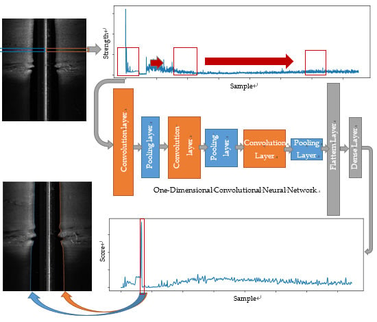
Deep learning algorithms have been widely applied in image recognition and classification [21,22,23,24]. The one-dimensional convolutional neural network (1D-CNN) is a deep learning algorithm for processing one-dimensional sequence data, and has been proven to be an effective recognition and classification method for one-dimensional sequence data [25,26]. After introducing the deep learning idea, algorithms can simulate the human brain, learn the variation feature of the local backscatter strength sequence, and fulfill the bottom tracking of side scan sonars. Therefore, on the basis of the recognition of side scan bottom data sequences through 1D-CNN, this paper presents a new real-time bottom tracking method for side scan sonar data. First, the operation theory of the side scan sonar and the characteristics of the side scan backscatter strength data are briefly introduced. Second, according to the variation features of backscatter strengths, the proposed 1D-CNN model is designed and then trained by using the established sample sets for recognizing bottom sequences. Third, the bottom tracking of side scan data is implemented by traversing each ping to use the trained model to detect the bottom data sequences. Lastly, the proposed method is validated in the experiment by using the measured side scan data.

2. Theory and Method

This chapter introduces the proposed real-time bottom tracking method using the 1D-CNN model. The basic theories of side scan operation and data characteristics, the recognition of bottom data sequences, and bottom tracking using the trained model will be explained successively.

2.1. Side Scan Sonar Operation and Data Characteristics

The operation of a side scan sonar is shown in Figure 1. The side scan sonar, which is usually a towfish, is towed by the survey vessel using a tow cable to get close to the seabed. The side scan sonar transducer projects a single wide sound beam (e.g., 50°, as shown in Figure 1) at the port and starboard sides. After the sound is projected from the side scan transducer, the transducer receives and records the backscatter strengths in the time sequence at the port and starboard sides, respectively, and these strengths are used to construct side scan sonar images. During the sound propagation, the backscatter strengths received from the water column are usually much lower than those received from the seabed, as shown in Figure 1. The special variations in signal levels (or backscatter strengths) when the sound arrives at the seabed serve as the basis for the bottom tracking of side scan sonar data. However, given the effects of sonar self-noise, suspended objects in the water column, and other instrumental and environmental factors, the many uncertainties in the sonar data introduce difficulties in bottom tracking.

As shown in Figure 1, the acoustic backscatter strengths of a ping have the following characteristics.

• The backscatter strengths in the water column area are much lower than those in the seabed area. The backscatter strengths in the water column area near the zero position are usually heavily affected by the self-noise of the side scan sonar.
• When the sound hits the seabed, the transducer receives higher echo signal intensities compared with those in the water column. Affected by the beam patterns and transmission losses [27], the strength sequences temporarily increase after the bottom position and, subsequently, decrease along with an increasing transmission length.
• The backscatter strength sequences of the port and starboard sides are almost symmetric at the zero position. However, the bottom tracking position may slightly differ due to the attitude of the side scan sonar and the seabed terrain slopes [19].

2.2. Recognition of Sonar Data Sequences Using 1D-CNN

When the sound hits the seabed, the local backscatter strength sequence shows a special variation feature, as illustrated in Figure 1. The proposed method uses the suitable 1D CNN model to recognize the bottom samples for bottom tracking. In this section, the positive and negative samples were first extracted to establish the sample sets. The sample sets were normalized and a 1D-CNN model was carefully designed and trained by using the sample sets.

2.2.1. Sampling

When using 1D-CNN to learn the variation features of the side scan data sequence, the one-ping backscatter data sequence should be divided into regional sub-sequences as samples, as illustrated in Figure 2. The sub-sequence/sample size should be properly selected to accurately reflect the variation characteristics, as discussed in Section 4.1. An improper sample size would cause the network to learn the wrong information and misjudge the results.

• A very large sample size cannot represent the special variation characteristics of backscatter strengths and
• A very small sample size can be easily affected by local noise.

To establish the sample sets, the positive and negative samples need to be selected from raw sonar backscatter strength data sequences. The positive samples can be detected using the traditional method with manual intervention, whereas the negative samples should contain the samples in the water column area, those containing noise, and those in the seabed area, as shown in Figure 2.

2.2.2. Normalization of Sonar Data Sequences

As shown in Figure 2, the samples are in various strength ranges and need to be normalized into the same range for the network training. These samples can be normalized by using the z-score to ensure that they are in the same range [28]. Given that the side scan data are usually recorded in a fixed range (e.g., 0 to 2¹⁶-1), the samples can be simply normalized by the equation below.

$$dB=\frac{dB}{Ma{x}_{dB}}\left(e.g.\frac{dB}{32767}\right).$$

(1)

After the normalization, the sample range should be normalized to (0~1), as shown in Figure 3.

2.2.3. Network

The bottom tracking of the side scan sonar data aims to recognize special bottom backscatter strength sequences, and can be fulfilled via the 1D-CNN recognition of the normalized data sequences.

1D-CNN is the one-dimensional version of common CNNs, which also contain input layers, convolution layers, pooling layers, and the output layers. Given the characteristics of our problem, the input layer of the 1D-CNN contains backscatter strength sequences, whereas the output layer contains the positive (1) and negative (0) results, as shown in Figure 4.

The input layer contains the one-dimensional normalized backscatter strength samples, and the median layers are combinations of convolution and pooling layers. The one-dimensional convolution operation s of the data sequences in discrete form is shown below.

$$s\left(t\right)=\left(d\ast w\right)\left(t\right)={\displaystyle \sum _{a=-\infty }^{\infty }d\left(a\right)}w\left(t-a\right)$$

(2)

where d is the input data sequence, w is the activation function, and t is the tth value of d.

The following rectified linear unit (ReLU) h is selected as the activation function for the convolution layers.

$$h_{w,b}\left(X\right)=\max \left(X·w+b,0\right)$$

(3)

where w and b are the trainable parameters, and X is the input data.

After the convolution and pooling layers, the flattened layer reshapes the tensors into vectors, whereas the fully-connected layer usually uses the ReLU to connect the output layer.

The last layer is the output layer, with the following activation sigmoid function σ:

$$\sigma (x)=\frac{1}{1+e^{-x}}$$

(4)

where x is the input data.

After each training loop, the loss function is used to calculate the difference between the predicted results and the ground truth. Given that the bottom tracking problem is a binary classification problem, the cross-entropy loss function is selected as the following loss function H.

$$H_{y_i}\left(y\right)=-{\displaystyle \sum _i{y}_i^{\prime }}\log \left(y_i\right)$$

(5)

where y_i is the predicted result and y_i^′ is the ground truth.

The root mean square propagation optimizer is chosen to update the parameters. After several loops, if the network learns the variation features of the samples properly, then the loss function would reach a stable low value, whereas the training and validation accuracies would reach stable high values. The well-trained 1D-CNN serves as the basis of the real-time bottom tracking method.

2.3. Bottom Tracking Using the Trained 1D-CNN

In this section, the trained network is used for the bottom tracking of the side scan data. The complete procedures of real-time bottom tracking are explained in detail, along with the auxiliary methods that can improve real-time performance and recognition accuracy.

2.3.1. Real-Time Bottom Tracking

By finding the first echo that reaches the seabed, the purpose of bottom tracking aims to accurately obtain the sonar height from the seabed, then geocode the sonar image, and fulfill other applications. Given that the trained network model can effectively understand the characteristics of the input samples, bottom tracking can be accomplished via the 1D-CNN recognition of local backscatter strength sequences. By traversing the ping data sequence in the propagation direction, the trained 1D-CNN recognizes the local backscatter strength sequence in each search window, and the predicted score of each local sequence can be obtained, as shown in Figure 5. The window size should be the same as the sample size.

The scores of the backscatter strength sequence in each search window are treated as the prediction results of the trained 1D-CNN. When the sound beam arrives at the seabed, a high score can be obtained by using the 1D-CNN prediction. Meanwhile, the scores of the data sequences in the other positions are far lower. Therefore, the maximum score position can be used to determine the bottom position of each ping.

Given the symmetry between the port and starboard data of each ping, a bottom tracking of the port and starboard data is carried out. The predicted port and starboard scores are then used to check the results and to achieve improved robustness to noise. The bottom tracking result of each ping is obtained on the basis of the port and starboard results. The complete bottom tracking procedures for each recorded ping is shown in Figure 6.

The bottom tracking accuracy of the survey line as obtained by 1D-CNN is calculated by using Equation (6) below.

$$acc=\frac{N_1}{N_0}$$

(6)

where N₁ is the number of successful-bottom-tracked pings and N₀ is the total number of pings.

2.3.2. Improving Speed: Narrow Search Range

The processing speed of the bottom tracking algorithm for each ping plays a key role in guaranteeing the real-time performance of the proposed method. Given the stringent hardware computing power requirements of the deep learning algorithm, the data sequences should be recognized in a limited search range instead of the whole ping. In the current common hardware platform (AMD R5-2600X CPU and GTX-2070 GPU), the relationship between different search scopes and corresponding times was analyzed and shown in Figure 7. The computing speed and search range are linearly dependent on the same hardware platform, which indicates that narrowing the search range can effectively improve the computing speed.

According to the continuity of the seabed terrain variation, the bottom tracking position (sonar height) of the former ping can be used as the initial search position, and the search range can be determined by the seabed terrain variation or bottom tracking position rate. The relationship between the bottom tracking position variation rate and search range is shown in

Table 1. Auto-Adapted Search Ranges Depending on the Bottom Position Variation.

Bottom Position Variation Rate r (Number of Samples/Ping)	r ≤ 5	5 < r < 10	10 < r < 20	20 < r < 40
Bottom position variation rate r (meter/ping)	r ≤ 0.2	0.2 < r < 0.4	0.4 < r < 0.8	0.8 < r < 1.6
Search range (number of samples)	20	40	80	160
Search range (meter)	0.8	1.6	3.2	6.4

. By combining the initial search position provided by the previous ping and the bottom tracking position variation rate between the previous pings, the search range of the proposed method can be adaptively controlled, to guarantee an excellent real-time performance.

2.3.3. Improving Accuracy: Sample Data Augmentation

The accuracy and abundance of samples are key in ensuring an accurate bottom sequence recognition. However, traditional sampling methods are time consuming and require manual intervention to ensure enough accuracy. During its application, the trained network could process other types of side scan sonar data in other seabed environments. The network needs to learn the features of the new data by continuously increasing the number of samples to improve the recognition accuracy. In this paper, a continuous increase of the samples was realized by using the learning ability of the network and few manual assistances, as shown in Figure 8.

As the number of samples increases, the recognition accuracy and robustness of the network can be further improved, and an accurate bottom tracking can be guaranteed.

3. Experiment and Results

To verify the validity and real-time performance of the proposed method, the side scan and multibeam data measured in Meizhou Bay, Fujian, China in 2012 were selected for the experiment, as shown in Figure 9. The coverage of the survey area was approximately 13.5 × 2.5 km², and the water depth ranged from 10 m to 40 m. The seabed sediments were mainly gravel and silt. According to the designed route, the measurements of the multibeam and side scan sonars were carried out successively in the same water area. In the multibeam measurement, Kongsberg EM 3002 with an operating frequency of 300 kHz, across-track beam aperture of 130° and maximum beam number of 131 was used. Meanwhile, in the side scan measurement, EdgeTech 4100P side scan sonar was towed at approximately 2 m underwater with an operating frequency of 500 kHz, maximum recorded slant range of 150 m (corresponding to 3751 sample numbers), vertical angular aperture of 50°, and horizontal angular aperture of 0.5°. The interval time between pings was 0.15 s on average. The side scan data were recorded in eXtended Triton Format (*.xtf) files, which only contained the backscatter strengths. The raw signal levels were unavailable, and the echoes were compensated with unknown gains.

The experiment was divided into the following stages.

• The experiment began by sampling, training, and bottom tracking of a small side scan survey line. Small sets of samples were initially extracted from the side scan data. Then the proposed 1D-CNN network model was trained to learn the variation features of the sample set. The training network was eventually used for bottom tracking, and the predicted value was compared with the artificially selected truth value.
• The trained network was validated by using additional side scan data of other survey lines to obtain the tracking results of other lines.

  •

  The bottom tracking result obtained by the proposed method was compared with those obtained by the traditional method.

  •

  The water depth predicted by using the bottom tracking results were compared with the ground truth (depths measured by the multibeam sonar).

  •

  The real-time performance of the proposed method was analyzed and validated via statistical analysis.

• Additional experiments on the side scan data with heavy noise and rich texture were conducted.

3.1. Network Model Establishment and Bottom Tracking

The experiment started with a small side scan survey line of 121 pings. The raw recorded (*.xtf) data was decoded, and the corresponding waterfall sonar image was constructed, as shown in Figure 10a. The bottom tracking results were processed by manual recognition, as shown in Figure 10b.

The positive sample sequences were selected as the bottom backscatter strength sequences from the side scan data, according to the corresponding bottom tracking position. Meanwhile, the negative sample sequences were uniformly selected in the water column and seabed area. The positive and negative samples constituted the sample set for the model training. Given that the survey line had 121 pings, the sample set contained 242 positive and 2662 negative samples, respectively.

The sample set was normalized, according to Equation (1), and was imported into the network as the input layer. The corresponding label (1: positive, 0: negative) was imported as the output layer. During the training, the samples were randomly divided into training and validation sets in a 70–30% proportion. The 1D-CNN (Figure 4) was trained to learn the variation features of the data samples. The training and validation accuracies improved as the training epoch increased, as shown in Figure 11.

As shown in Figure 11, the training accuracy gradually improved as the training epoch increased, and eventually reached a stable value of 100% after approximately 40 training epochs. The validation accuracy fluctuated in 10 training epochs and reached a stable value after 20 epochs. The training and validation losses gradually decreased along with an increasing training epoch, and eventually decreased to 0. For the small sample set of the selected survey line, the network model proposed in this paper can effectively learn the features of the positive and negative samples, and accurately recognize them after training, which is the basis for the real-time bottom tracking of the survey line.

Based on the trained network model, each ping of the survey line was bottom tracked following the procedure illustrated in Figure 6. The bottom tracking results of the port and starboard side scan data were then processed (Figure 5) and compared with each other (Figure 12a). The corresponding bottom tracking result can be displayed in the side scan waterfall image (Figure 12b).

The bottom tracking results of the port and starboard data were highly consistent with each other, and all bottom position differences were less than four samples (0.16 m) because the seabed topography of the survey water area was relatively flat. Moreover, the tracking results in the waterfall diagram were highly intuitive to show the edges of the port and starboard seabed area, which agreed with the visual results. The comparison between the bottom tracking results and manual ones showed that the bottom tracking accuracy can reach 100% on the training survey line. These results prove the validity of the proposed bottom tracking method.

3.2. Method Validation and Comparison

To validate the generalization of the trained model and the effectiveness of the proposed method for the side scan data of other survey lines in the test area, the trained model was used to recognize unknown data for the bottom tracking of other survey lines.

3.2.1. Validation on a Larger Survey Line

The side scan data of a long survey line with 13,504 pings were used for the validation. The survey line spanned the seabed of two different sediments, which appeared as the clearly lighter and darker areas in the side scan image, as shown in Figure 13b. At the joint area of the two sediments, the seabed topography rapidly changed, as shown in Figure 13c. Based on the 1D-CNN model that was trained by using the sample set of a small survey line, the bottom tracking of the validation survey line was processed, and the results are shown in Figure 13. During the processing, the search ranges of each ping were self-adapted to improve the speed, according to Table 1.

As shown in Figure 13a, the port and starboard results were consistent with each other, and the bottom tracking lines coincided with the edges of the port and starboard seabed in the waterfall image shown in Figure 13b. After removing the missing ping data of this survey line, the accuracy of the bottom tracking results reached 99.5%. In the area where the seabed terrain changed rapidly, the proposed bottom tracking method with auto-adapt search ranges still achieved good tracking results, which proved the validity of the proposed method in both flat and rugged seabed environments.

3.2.2. Comparison with Other Bottom Tracking Methods

To compare the proposed method with traditional methods, the survey line was processed by using the last peak method [19]. For real-time processing, the last peak method was used without post-processing, including Kalman filtering. The tracking results obtained by both methods are shown in Figure 14.

The bottom tracking results obtained by using these two methods were consistent in most positions. However, the results obtained by the traditional method based on the numeric features were sensitive to noise, such as water column noise and seabed objects., so the results could possibly be inaccurate without post-processing. As for the proposed method, by training the sample sets, the network could properly learn the variation feature of the backscatter strength sequences, and show better robustness to noise. As more samples were learned, the 1D-CNN could more accurately recognize the side scan data. The comparison proved the validity and performance of the proposed method.

3.2.3. Comparison Between the Bottom Tracking Depths and Ground Truth (Manual Annotations)

The manual annotations of bottom positions were used as the ground truth for the bottom tracking results of the side scan sonar data. Additionally, the bathymetric data measured by the multibeam sonar can be regarded as good references for the bottom tracking results. The depth of the side scan sonar sensor can be obtained by using its depth sensor, and the sonar height can be calculated by using the bottom tracking results. Therefore, the depth D of the corresponding seabed can be calculated using the equation below.

$$D=\frac{n\times t\times v}{2}+d$$

(7)

where n is the nth sample detected as bottom, t is the sampling interval time, v is the sound velocity, and d is the side scan sonar depth.

The digital elevation model was constructed by using the multibeam bathymetric data in the selected survey marine area (Figure 13c), as shown in Figure 15a. The track line of the multibeam data was extracted, and the corresponding water depths are shown in Figure 15d. The seabed depths of the side scan survey line that corresponded to the multibeam survey line were calculated by using the manual annotation and the predicted data, as shown in Figure 15b,c.

In the same water area, the seabed depths measured by the multibeam sonar (Figure 15d), those calculated by using manual annotations (Figure 15b), and the bottom tracking results (Figure 15c) were consistent with each other. The significant terrain fluctuations in the middle of the region coincided with the seabed variation shown in Figure 13c. Given that the multibeam and side scan data were measured at different times and that the multibeam data were not post-processed, the depths of the multibeam data had some errors and showed slight deviations from the depths calculated by using the side scan data. The terrain variation trends were consistent with each other, which proves the accuracy of the bottom tracking data.

The depth errors between the predicted and manual annotated depths were fitted using a normal curve with the mean μ equal to 1.21 cm and standard deviation σ equal to 8.57 cm, as shown in Figure 15e. Given that the errors of manual annotations were within ±3 samples (corresponding to ±12.0 cm), the depth errors were less than two times the error (i.e., 24.0 cm) can be acceptable. By statistical analysis, the depth errors (Figure 15e) within ±24.0 cm are in a 99.44% proportion. Thereby, the accuracy of the bottom tracking results compared with manual annotations is 99.44%.

3.2.4. Real-Time Experiment

To verify the real-time performance of the proposed method, the spend times of each ping were recorded during the bottom tracking experiment. The bottom tracking results and time sequences are shown in Figure 16a,b, respectively, whereas the spend times were statistically analyzed to evaluate the real-time performance, as shown in Figure 16c.

Given the auto-adapt search ranges used in the bottom tracking experiment, the spend times of each ping changed along with the variation rate of the seabed terrain. The spend times of each ping were fitted by using the normal distribution curve with a mean μ of 82.1 cm and a variance σ of 0.12 cm. According to the statistical analysis results, the confidence bound of the side scan sampling interval time of each ping (150 ms) was 99.9%, which suggests a 99.9% possibility for the calculation time of each ping to be shorter than the sampling interval time. Moreover, it is guaranteed that, given the number of predicted sample sequences being less than 60, the calculation speed is always less than 150 ms, where 150 ms is the interval time between two pings. The statistical results proved the real-time feasibility of the proposed method.

Moreover, if the prior depth range is known, then the search range of each ping would be smaller. Moreover, with better hardware and multi-thread computing, the calculation speed would be improved, as discussed in Section 4.4.

3.3. Bottom Tracking of Side Scan Data with Noise and Rich Texture

To obtain the bottom tracking results of the other survey lines in the experimental area, data augmentation was applied on the sample sets as more survey lines were processed, as shown in Figure 8. The characteristic side scan data with large noise, rich seabed texture, and artificial targets were carefully processed and analyzed, as shown in Figure 17. The recorded side scan data contained missing pings, which had no backscatter strengths or very low backscatter strengths, as shown in yellow rectangles in Figure 17.

Figure 17a shows that the noises in the water column are relatively large. In the red rectangular area, the noises in the water column made the seabed and water column data indistinguishable, or made the edge variation of the seabed abnormal. The bottom tracking accuracy of this survey line as obtained by 1D-CNN was 97.3% with a 2.0% miss-ping rate. The accuracy excluding the missing pings was 99.3%.

Figure 17b shows that the seabed has rich textures and that some noise can be observed in the water column. The backscatter strength variation of the complex seabed texture would result in clear light and shade areas, which would interfere with bottom tracking. The bottom tracking accuracy of this survey line as achieved by 1D-CNN was 93.1% with a 6.1% miss-ping rate. The accuracy excluding the missing pings was 99.1%.

Figure 17c shows that the seabed contains artificial targets, such as submarine pipelines. These artificial targets can also cause light and shade areas in the side scan image, which would significantly affect bottom tracking. The bottom tracking accuracy of this survey line as achieved by 1D-CNN was 94.5% with a 4.9% miss-ping rate. The accuracy excluding the missing pings was 99.4%, as shown in

Table 2. Bottom Tracking Accuracies of the Survey Lines Shown in Figure 17.

Survey Line (in Figure 17)	Tracking Accuracy Using 1D-CNN	Miss-Ping Rate	Tracking Accuracy Excluding the Missing Pings
a	97.3%	2.0%	99.3%
b	93.1%	6.1%	99.1%
c	94.5%	4.9%	99.4%

.

As shown in Table 2, by means of sample data augmentation, mutual inspection of the port and starboard results, and auto-adapt search ranges, the proposed method can guarantee the bottom tracking accuracy of the side scan data with large amounts of noise, a rich seabed texture, and artificial targets as well as simultaneously realize real-time calculation performance. The average bottom tracking accuracy of the overall testing survey lines as achieved by 1D-CNN was 94.7% with a 4.5% miss-ping rate. The tracking accuracy excluding the missing pings was 99.2%. The experiments proved that the proposed method has high robustness to noise, and can yield accurate results in complex seabed conditions.

4. Discussion

4.1. Determination of the Sample Size

Sample size is an important factor in accurately recognizing the bottom data samples and further realizing bottom tracking of the side scan data. If the sample size is too large, then the samples cannot represent the special variation characteristics of the bottom data sequences. However, if the sample size is too small, then the samples can be easily affected by local noise. For a better comparison, bottom tracking experiments were conducted with sample sizes of 10, 20, 40 (chosen in this paper), and 100, as shown in

Table 3. Comparison of results obtained under different sample sizes after a 50-epoch training with 242 positive samples and 2662 negative samples.

Sample Size (Number of Recorded Samples)	Sample Size (m)	Training Accuracy (%)	Validation Accuracy (%)	Bottom Tracking Accuracy (%)
10	0.4	98.1	98.6	0.0
20	0.8	99.7	100	98.3
40	1.6	99.9	100	100
100	4.0	100	100	46.3

.

As shown in Table 3, when the sample size was as small as 10, although the training and validation accuracies were high enough, the bottom tracking accuracy was 0%, which suggests that the variation characteristics of the samples can be easily affected by noise. When the sample size was as large as 20, the training and validation accuracies were improved, and the bottom tracking accuracy reached as high as 98.3%. When the sample size was 40 (as used in this paper), the training and validation accuracies were further improved, and the bottom tracking accuracy increased to 100%, which suggests that the samples can accurately reflect the variation characteristics of backscatter strengths. However, when the sample size was 100, although the training and validation accuracies were 100%, the bottom tracking accuracy was only 46.3%, which suggests that the samples cannot properly reflect the variation characteristics of bottom backscatter strengths. The comparison results reveal that the proper sample size of the window should be 40 (as used in this paper) for the side scan sonar.

4.2. Net Comparison

To compare the performance of different networks, given the characteristics of the input sample data, the networks of different layers were established, trained, and used in bottom tracking experiments. The results are shown in

Table 4. Comparison of Results Obtained by Using the Networks of Different Layers.

Network Layer	Training Accuracy (%)		Validation Accuracy (%)	Bottom Tracking Accuracy (%)	Time per Ping (s)
	10 Epochs	20 Epochs
6	89.5	97.3	98.1	90.0	0.24
8	98.4	99.8	99.6	95.0	0.30
10	98.6	99.6	100	98.3	0.35

.

As seen from Table 4, with a sufficient number of samples, the deeper networks demonstrated better learning rates and higher training, validation, and bottom tracking accuracies, but required a longer calculation time. Meanwhile, each convolution operation would further reduce the data size. Therefore, the maximum number of network convolution layers was limited due to the limitations in the input data size. In this paper, a network of 10 layers was adopted (Figure 4).

4.3. Exceptional Situations

The validity of the proposed method was proven by conducting experiments using side scan data collected from Meizhou Bay. However, in some special cases when the backscatter strengths of sea bottom cannot be recognized, the proposed method may return invalid results. These possible exceptional situations are:

• The sonar altitude to the seabed is too low (less than 5 m). When the sonar is too close to the seabed, the variation characteristics of the bottom sequences would be overridden by the sonar self-noises in the water column area, which would make bottom tracking impossible. This situation can be avoided by controlling the sonar altitude within the proper range.
• The backscatter strengths of the seabed are too weak, and are no different from those of the water column area. This situation may be caused by the low-energy-level sonar emission, special sediment types, or maloperation of sonar instruments. In this situation, the backscatter strengths of the seabed are almost in the same range as those of the water column, cannot reflect the variation characteristics of the bottom echo sequences, and would make bottom tracking very difficult. This situation can be avoided by increasing the sound energy level, using the different-frequency sonars, and ensuring careful manual operation.

4.4. Other Methods for Improving Efficiency

The proposed method realizes bottom tracking of side scan data based on 1D-CNN recognition. In addition to the methods mentioned in this paper, some other ways to improve the efficiency of the proposed method include:

• Define the depth range in advance. For the pre-surveyed water area, the previous bathymetric data can be used to define the depth range. The pre-known depth range can be used to control the detection ranges of the side scan data and to validate the bottom tracking results. Therefore, the pre-defined depth range can improve the calculation efficiency of the proposed bottom tracking method.
• Improve the computing hardware. Given the high computing ability requirements of the deep learning algorithm, using better computing hardware can improve the calculation of the proposed method and reduce the bottom tracking time of each side scan ping. With the development of sonar technologies, given that sonars will have higher sample rates, a better computing hardware can improve the calculation efficiency of the proposed bottom tracking method.

4.5. Development of Modern Scanning Sonars

With the development of modern sonar technologies including interferometry, the newest scanning sonar could not only obtain sonar images but also bathymetric data [29] including the following.

• Kongsberg GeoSwath sonars can simultaneously offer swath bathymetry and side scan seabed mapping with sufficient accuracy.
• Teledyne Blueview’s 3D multibeam scanning sonar can create high-resolution and laser-like imagery of underwater areas, structures, and objects of interest.

Although these sonars have many advantages, they are only used by a limited number of companies and research institutions because of their high cost.

The traditional side scan sonar remains one of the most widely used marine survey instruments because of its very low cost. Moreover, modern data process algorithms may provide new abilities for the traditional side scan sonar. In this paper, by using a real-time bottom tracking algorithm, the side scan sonar can measure the seabed depth. This enhances the potential applications of the side scan sonar.

4.6. Handling of Important Issues

The following important issues should be noted.

Low SNR. Our method processes side scan data that have been compensated and converted in fixed ranges when most information (e.g., the original signal level and time-varied gain) is unavailable. Under this situation, the echo intensities are almost in the same range. When the SNR is very small, the echo intensities of the bottom can be affected by noise, but the variation features remain. We believe that our method can process side scan data with very small SNR after training of the corresponding samples.

Obstacles in the water column. When obstacles (e.g., the fish school) exist above the seabed, the fishes can be easily distinguished by using the trained 1D-CNN with enough negative samples (i.e., fishes). By training with all types of obstacle samples, the network can distinguish the bottom, the fishes, and the other obstacle targets from one another. Moreover, when the bottom continuity hypothesis fails, our method will automatically search for the new bottom position.

Reproducibility. Each step of our method is described in detail, including how to create the samples from the recorded side scan data, how to design a suitable 1D-CNN, how to train the network, and how to use the proposed bottom tracking method. In the experiment, we demonstrate our complete processing procedure, including the sampling, training, and bottom tracking. We believe that the reader can easily reproduce our results by using their own side scan data.

5. Conclusions

Based on the 1D-CNN recognition of bottom backscatter strength sequences, this paper develops a high-accuracy and real-time bottom tracking method of side scan sonar data. This method was validated by using the measured side scan data from Meizhou Bay, and the validity of each step of this method was proven. The side scan sonar data from the experimental area were bottom tracked by using the proposed method, and the average bottom tracking accuracy reached 94.7% with a 4.5% miss-ping rate, and 99.2% excluding the missing data. The experimental results showed that the proposed method is highly robust to the effects of noise, rich seabed texture, and artificial targets and proved its accuracy and real-time performance. Our method can process side scan data in field measurements (i.e., when the operator has no control over the SNR, or when fishes or obstacles are present in the water column, or in analogue simulations by using the recorded data), and in post-processing (i.e., when the recorded data only contain compensated and converted backscatter strengths). The proposed method also demonstrates that the real-time sound is possible by using the side scan sonar, which may further expand the applications of side scan sonars.