Adaptive Least-Squares Collocation Algorithm Considering Distance Scale Factor for GPS Crustal Velocity Field Fitting and Estimation


Abstract
:
1. Introduction
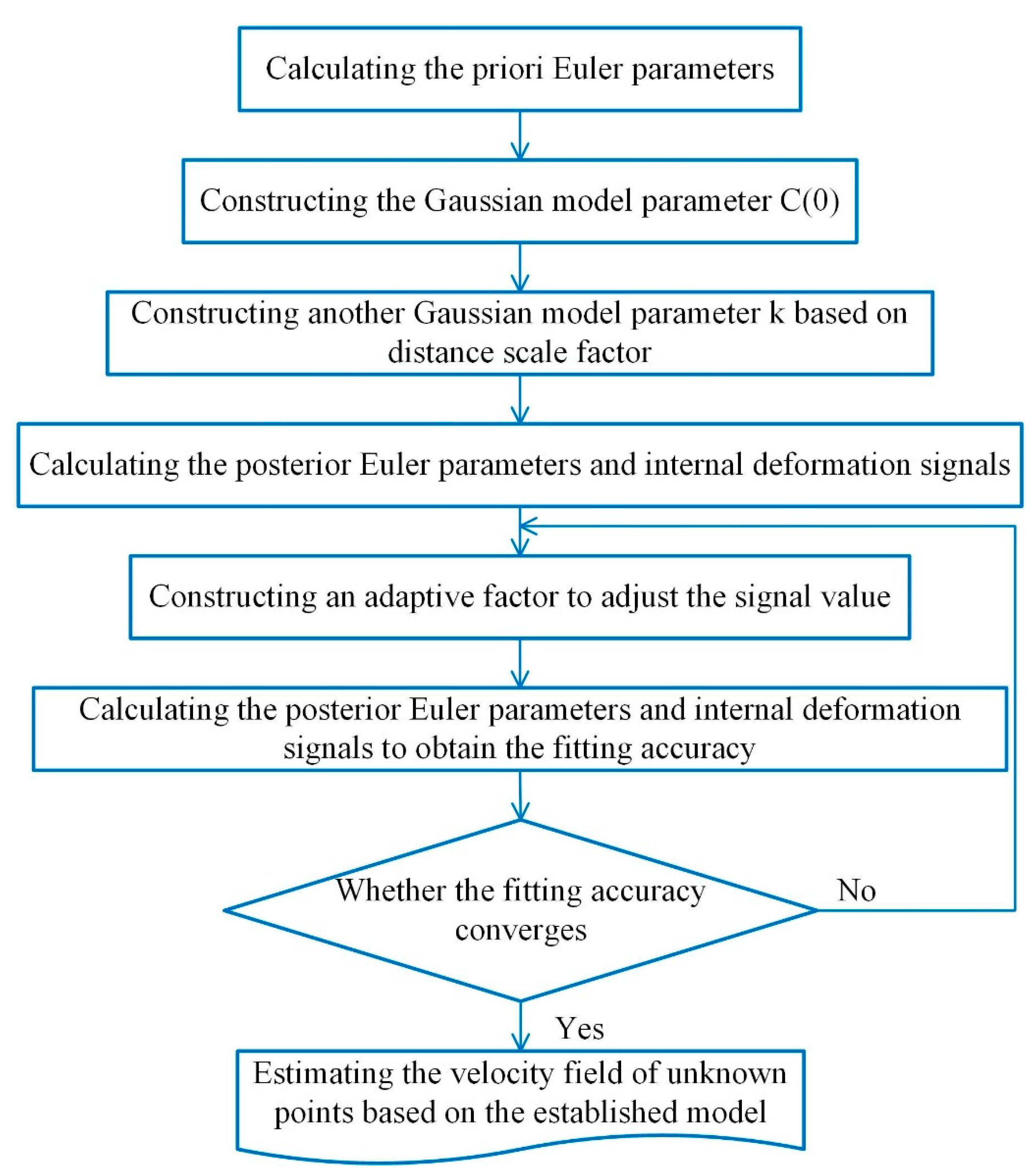
2. Methods
2.1. Traditional LSC Algorithm
2.2. Considering Distance Scale Factor
2.3. Adaptive Collocation
2.4. Fusion Algorithm
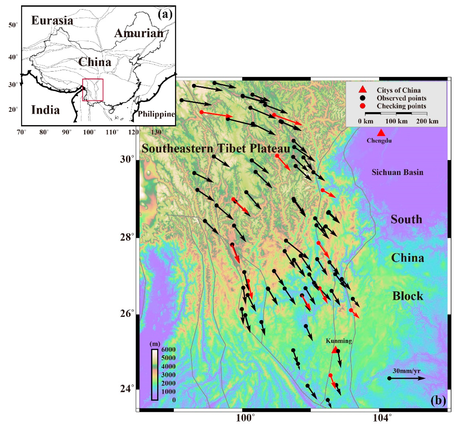
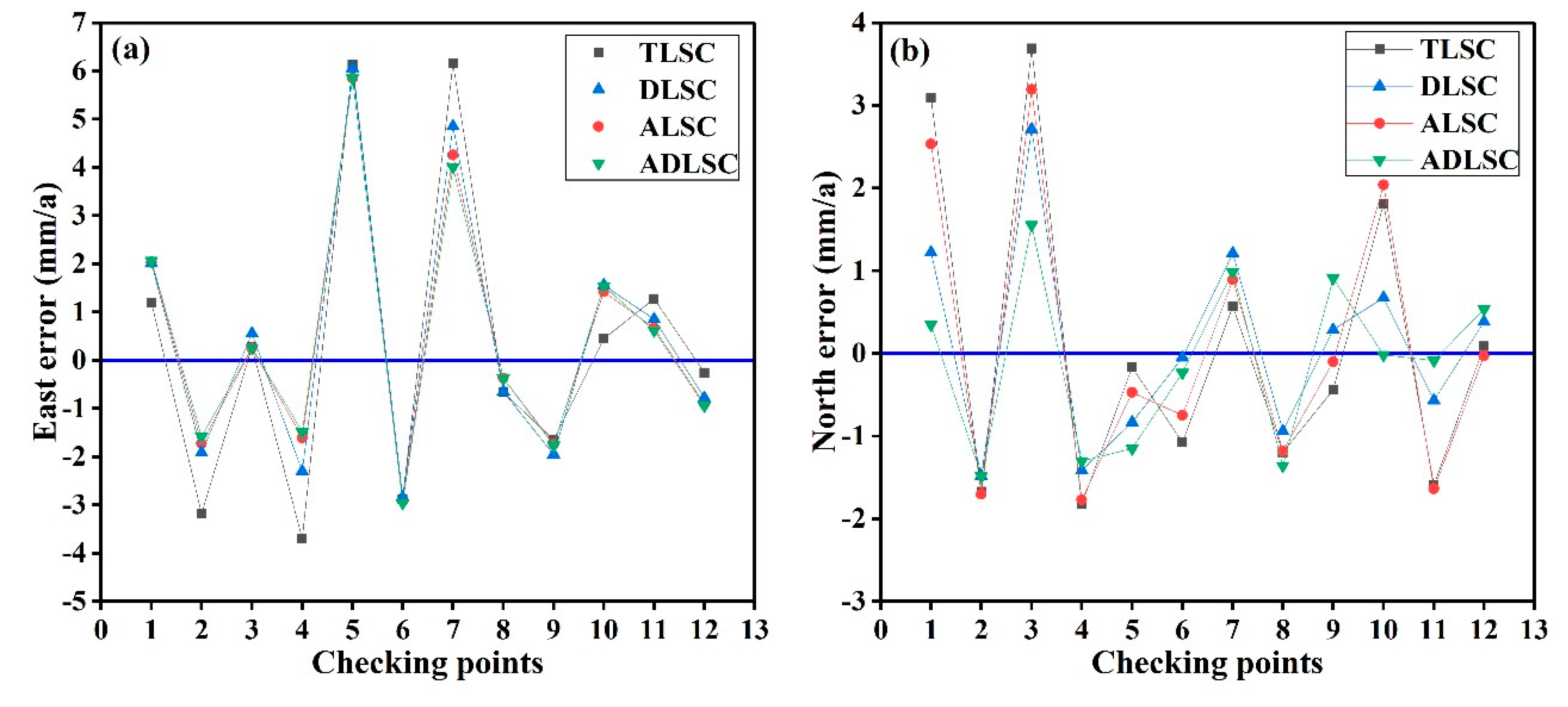
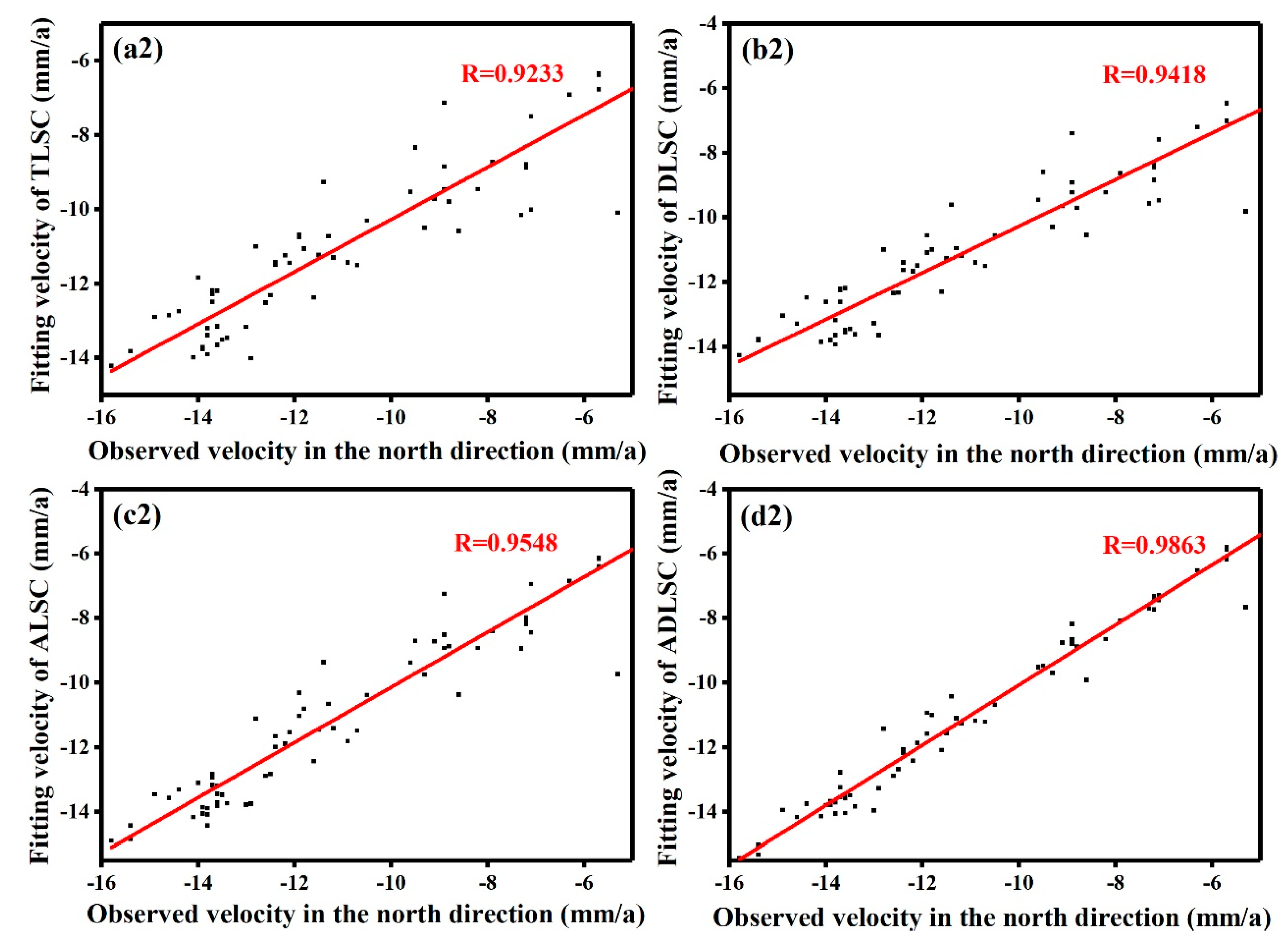
3. Results and Analysis
4. Discussion
4.1. Influence of Noise Levels on the New Algorithm
4.2. Influence of Randomly Selected Checking Points on Algorithms
4.3. Determination of the Optimal Distance Scale Factor of the New Algorithm
4.4. Advantage of the New Algorithm for Treating Functional Model Error
5. Conclusions
Author Contributions
Funding
Acknowledgments
Conflicts of Interest
References
- Mansurov, A.N. A continuum model of present-day crustal deformation in the Pamir-Tien Shan region constrained by GPS data. Russ. Geol. Geophys. 2017, 58, 787–802. [Google Scholar] [CrossRef]
- Yu, B.H.; Guan, Z.; Xu, X.F.; Yang, L.Q. The Application of an Improved Multi-surface Function Based on Earth Gravity Field Model in GPS Leveling Fitting. In Communications in Computer and Informationence; Springer: Berlin/Heidelberg, Germany, 2013. [Google Scholar]
- Gonçalves, B.M.F.; Afonso, M.M.; Coppoli, E.H.D.R.; Coppoli, E.H.R.; Ramdane, B.; Marechal, Y.; Vollaire, R.; Krähenbühl, L. Comparison of Natural and Finite Element Interpolation Functions Behavior at Interface between Different Mediums. Int. J. Numer. Model. Electron. Netw. Devices Fields 2017, 31, e2230. [Google Scholar] [CrossRef]
- Martín, A.; Núñez, M.A.; Gili, J.A.; Anquela, A.B. A comparison of robust polynomial fitting, global geopotential model and spectral analysis for regional–residual gravity field separation in the Doñana National Park (Spain). J. Appl. Geophys. 2011, 75, 327–337. [Google Scholar] [CrossRef]
- Zeng, A.M.; Liu, G.M.; Qin, X.P.; Tang, Y.Z. Research on the horizontal velocity motion field of China’s continental crust by collocation method. Bull. Surv. Mapp. 2012, (Suppl. 1), 11–15. (In Chinese) [Google Scholar]
- Wu, Y.Q.; Jiang, Z.S.; Yang, G.H.; Wei, W.X.; Liu, X.X. Comparison of GPS strain rate computing methods and their reliability. Geophys. J. Int. 2011, 185, 703–717. [Google Scholar] [CrossRef]
- Moritz, H. Interpolation and Prediction of Gravity and their Accuracy; Air Force Cambridge Research Labs Lg Hanscom Field Mass: Bedford, MA, USA, 1962. [Google Scholar]
- Krarup, T. A Contribution to the Mathematical Foundation of Physical Geodesy; Cpenhagen Danish Geodetic Institute: Copenhagen, Denmark, 1969. [Google Scholar]
- El-Fiky, G.S.; Kato, T. Continuous distribution of the horizontal strain in the Tohoku district, Japan, predicted by least-squares collocation. J. Geodyn. 1998, 27, 213–236. [Google Scholar] [CrossRef]
- Gamal, E.F. GPS-derived velocity and crustal strain field in the Suez-Sinai area, Egypt. Bull. Earthq. Res. Inst. Univ. Tokyo 2005, 80, 73–86. [Google Scholar]
- Wu, J.C.; Tang, H.W.; Chen, Y.Q.; Li, Y.X. The current strain distribution in the north china basin of eastern china by least-squares collocation. J. Geodyn. 2006, 41, 462–470. [Google Scholar] [CrossRef]
- Jiang, G.Y.; Xu, C.J.; Wen, Y.M.; Xu, X.W.; Ding, K.H.; Wang, J.J. Contemporary tectonic stressing rates of major strike-slip faults in the Tibetan Plateau from GPS observations using least-squares collocation. Tectonophysics 2014, 615–616, 85–95. [Google Scholar] [CrossRef]
- Wu, Y.Q.; Jiang, Z.S.; Zhao, J.; Liu, X.X.; Wei, W.X.; Liu, Q.; Li, Q.; Zou, Z.Y.; Zhang, L. Crustal deformation before the 2008 Wenchuan Ms8.0 earthquake studied using GPS data. J. Geodyn. 2015, 85, 11–23. [Google Scholar] [CrossRef]
- Qu, W.; Lu, Z.; Zhang, M.; Zhang, Q.; Wang, Q.L.; Zhu, W.; Qu, F.F. Crustal strain fields in the surrounding areas of the ordos block, central china, estimated by the least-squares collocation technique. J. Geodyn. 2017, 106, 1–11. [Google Scholar] [CrossRef]
- Qu, W.; Lu, Z.; Zhang, Q.; Hao, M.; Wang, Q.L.; Qu, F.F.; Zhu, W. Present-day crustal deformation characteristics of the southeastern Tibetan Plateau and surrounding areas by using GPS analysis. J. Asian Earth Sci. 2018, 163, 22–31. [Google Scholar] [CrossRef]
- Yang, Y.X.; Zhang, J.Q.; Zhang, L. Fitting estimation based on variance component estimation and its application in GIS error correction. J. Surv. Mapp. 2008, 37, 152–157, (In Chinese with English abstract). [Google Scholar]
- Wang, H.D.; Chai, H.Z.; Pei, T.Z.; Ruan, C.W. Comparison of two trend surface detection algorithms for multibeam sounding anomalies. Ocean Bull. 2010, 29, 182–186, (In Chinese with English abstract). [Google Scholar]
- Li, C.R.; Yue, D.J.; Yuan, B.; Xu, Y. Application of nine-parameter model based on least squares collocation in three-dimensional coordinate transformation. Mapp. Spat. Geogr. Inf. 2014, 37, 193–196, (In Chinese with English abstract). [Google Scholar]
- Mao, Q.Z.; Zhang, L.; Li, Q.Q.; Hu, Q.W.; Yu, J.W.; Feng, S.J.; Ochieng, W.; Gong, H.L. A Least Squares Collocation Method for Accuracy Improvement of Mobile LiDAR Systems. Remote Sens. 2015, 7, 7402–7424. [Google Scholar] [CrossRef]
- Zhao, Q.L.; Xu, X.Y.; Forsberg, R.; Strykowski, G. A Least Squares Collocation Method for Accuracy Improvement of Mobile LiDAR Systems. Remote Sens. 2018, 10, 1951. [Google Scholar] [CrossRef]
- Gao, X.B. Aviation Gravity Data Processing and its Application Research. Ph.D. Thesis, PLA Information Engineering University, Zhengzhou, China, 2013. (In Chinese with English abstract). [Google Scholar]
- Moritz, H. Least Squares Collocation. Rev. Geophys. Space Phys. 1978, 16, 421–430. [Google Scholar] [CrossRef]
- Yang, Y.X.; He, H.; Xu, G. Adaptively robust filtering for kinematic geodetic positioning. J. Geod. 2001, 75, 109–116. [Google Scholar] [CrossRef]
- Yang, Y.X.; Gao, W. An Optimal Adaptive Kalman Filter. J. Geod. 2006, 80, 177–183. [Google Scholar] [CrossRef]
- Yang, Y.X.; Zeng, A.M.; Zhang, J.Q. Adaptive collocation with application in height system transformation. J. Geod. 2009, 83, 403–410. [Google Scholar] [CrossRef]
- Niu, Z.J.; Min, W.; Sun, H.R.; Sun, J.Z.; Gan, W.J.; Xue, G.J.; Hao, J.X.; Xin, S.H.; Wang, Y.Q.; Wang, Y.X.; et al. Contemporary velocity field of crustal movement of Chinese mainland from Global Positioning System measurements. Chin. Sci. Bull. 2005, 50, 939–941. [Google Scholar] [CrossRef]
- Gan, W.J.; Li, Q.; Zhang, R.; Shi, H.B. Construction and Application of Tectonic Environment Monitoring Network in Mainland China. Eng. Res. Eng. Interdiscip. Persp. 2012, 4, 324–331, (In Chinese with English abstract). [Google Scholar]
- Liang, S.M.; Gan, W.J.; Shen, C.Z.; Xiao, G.R.; Liu, J.; Chen, W.T.; Ding, X.G.; Zhou, D.M. Three-dimensional velocity field of present-day crustal motion of the Tibetan Plateau derived from GPS measurements. J. Geophys. Res. Solid Earth 2013, 118, 1–11. [Google Scholar] [CrossRef]
- Zhang, P.Z.; Gan, W.J.; Shen, Z.K. A coupling model of rigid-block movement and continuous deformation: Patterns of the present-day deformation of China’s continent and its vicinity. Acta Geol. Sin. 2005, 79, 748–756. [Google Scholar]


| Algorithms | Fitting Points RMS (mm/a) | Checking Points RMS (mm/a) | Running Time (s) | ||
|---|---|---|---|---|---|
| (E) | (N) | (E) | (N) | ||
| TLSC | 2.43 | 1.32 | 3.21 | 1.86 | 1.29 |
| DLSC | 2.00 | 1.19 | 2.61 (18.7%) | 1.73 (6.9%) | 0.81 |
| ALSC | 2.15 | 0.96 | 2.82 (12.1%) | 1.24 (33.3%) | 1.42 |
| ADLSC | 1.96 | 0.54 | 2.57 (19.9%) | 1.03 (44.6%) | 1.05 |
| Algorithms | Noise Levels () | RMS (mm/a) (Fitting Points) | RMS (mm/a) (Check Points) | ||
|---|---|---|---|---|---|
| (E) | (N) | (E) | (N) | ||
| TLSC | 0.1 | 1.82 | 0.64 | 2.42 | 1.04 |
| 1 | 2.08 | 0.91 | 2.73 | 1.18 | |
| 10 | 2.43 | 1.32 | 3.21 | 1.86 | |
| ALSC | 0.1 | 2.15 | 0.96 | 2.82 | 1.24 |
| 1 | 2.15 | 0.96 | 2.82 | 1.24 | |
| 10 | 2.15 | 0.96 | 2.82 | 1.24 | |
| Algorithms | Fitting Points RMS (mm/a) | Checking Points RMS (mm/a) | Running Time (s) | ||
|---|---|---|---|---|---|
| (E) | (N) | (E) | (N) | ||
| TLSC | 2.32 | 1.35 | 2.81 | 2.00 | 1.29 |
| DLSC | 1.98 | 1.09 | 2.37 (15.7%) | 1.79 (10.5%) | 0.81 |
| ALSC | 2.12 | 0.99 | 2.55 (9.3%) | 1.72 (14.0%) | 1.42 |
| ADLSC | 1.94 | 0.68 | 2.34 (16.7%) | 1.36 (32.0%) | 1.05 |
| Algorithms | Fitting Points RMS (mm/a) | Checking Points RMS (mm/a) | Running Time (s) | ||
|---|---|---|---|---|---|
| (E) | (N) | (E) | (N) | ||
| TLSC | 2.38 | 1.59 | 2.84 | 1.88 | 1.29 |
| DLSC | 1.89 | 1.42 | 2.32 (18.3%) | 1.56 (17.0%) | 0.81 |
| ALSC | 2.01 | 1.29 | 2.71 (4.6%) | 1.35 (28.2%) | 1.42 |
| ADLSC | 1.87 | 1.14 | 2.30 (19.0%) | 1.11 (41.0%) | 1.05 |
| Noise Levels () | E (mm/a) | N (mm/a) | ||
|---|---|---|---|---|
| ALSC | ADLSC | ALSC | ADLSC | |
| 0.1 | 18.4682 | 2.3495 (87.3%) | 3.6667 | 2.0740 (43.4%) |
| 1 | 5.4206 | 0.8802 (83.8%) | 1.2534 | 1.1009 (12.2%) |
| 10 | 2.7854 | 0.8020 (71.2%) | 1.0777 | 0.8921 (17.2%) |
© 2019 by the authors. Licensee MDPI, Basel, Switzerland. This article is an open access article distributed under the terms and conditions of the Creative Commons Attribution (CC BY) license (http://creativecommons.org/licenses/by/4.0/).
Share and Cite
Qu, W.; Chen, H.; Liang, S.; Zhang, Q.; Zhao, L.; Gao, Y.; Zhu, W. Adaptive Least-Squares Collocation Algorithm Considering Distance Scale Factor for GPS Crustal Velocity Field Fitting and Estimation. Remote Sens. 2019, 11, 2692. https://doi.org/10.3390/rs11222692
Qu W, Chen H, Liang S, Zhang Q, Zhao L, Gao Y, Zhu W. Adaptive Least-Squares Collocation Algorithm Considering Distance Scale Factor for GPS Crustal Velocity Field Fitting and Estimation. Remote Sensing. 2019; 11(22):2692. https://doi.org/10.3390/rs11222692
Chicago/Turabian StyleQu, Wei, Hailu Chen, Shichuan Liang, Qin Zhang, Lihua Zhao, Yuan Gao, and Wu Zhu. 2019. "Adaptive Least-Squares Collocation Algorithm Considering Distance Scale Factor for GPS Crustal Velocity Field Fitting and Estimation" Remote Sensing 11, no. 22: 2692. https://doi.org/10.3390/rs11222692
APA StyleQu, W., Chen, H., Liang, S., Zhang, Q., Zhao, L., Gao, Y., & Zhu, W. (2019). Adaptive Least-Squares Collocation Algorithm Considering Distance Scale Factor for GPS Crustal Velocity Field Fitting and Estimation. Remote Sensing, 11(22), 2692. https://doi.org/10.3390/rs11222692