Enhanced Feature Extraction for Ship Detection from Multi-Resolution and Multi-Scene Synthetic Aperture Radar (SAR) Images

Abstract

Independent of daylight and weather conditions, synthetic aperture radar (SAR) images have been widely used for ship monitoring. The traditional methods for SAR ship detection are highly dependent on the statistical models of sea clutter or some predefined thresholds, and generally require a multi-step operation, which results in time-consuming and less robust ship detection. Recently, deep learning algorithms have found wide applications in ship detection from SAR images. However, due to the multi-resolution imaging mode and complex background, it is hard for the network to extract representative SAR target features, which limits the ship detection performance. In order to enhance the feature extraction ability of the network, three improvement techniques have been developed. Firstly, multi-level sparse optimization of SAR image is carried out to handle clutters and sidelobes so as to enhance the discrimination of the features of SAR images. Secondly, we hereby propose a novel split convolution block (SCB) to enhance the feature representation of small targets, which divides the SAR images into smaller sub-images as the input of the network. Finally, a spatial attention block (SAB) is embedded in the feature pyramid network (FPN) to reduce the loss of spatial information, during the dimensionality reduction process. In this paper, experiments on the multi-resolution SAR images of GaoFen-3 and Sentinel-1 under complex backgrounds are carried out and the results verify the effectiveness of SCB and SAB. The comparison results also show that the proposed method is superior to several state-of-the-art object detection algorithms.

1. Introduction

Due to the all-weather, all-day characteristics, SAR has become one of the important means of earth observation [1], such as vehicle detection [2], river detection [3] and image recognition [4,5]. Through airborne and spaceborne SAR, a large number of high resolution SAR ocean images can be obtained. Ship detection from SAR images is one of the important research directions of SAR image interpretation, and is widely used in military and civilian fields. The traditional method for ship detection from SAR images includes statistical distribution-based methods [6,7,8,9], multi-scale-based methods [10], template matching [11] and multiple/full polarization-based methods [12,13]. These methods highly rely on the distributions of sea clutters and the predefined thresholds [14,15,16]. At the same time, traditional ship detection systems usually consist of several steps, including land masking, preprocessing, prescreening and discrimination [17,18]. The multi-step operation mode of the traditional methods leads to time-consuming and low robustness of detection. Deep learning has also been applied to SAR ship detection [19,20,21,22,23,24,25].

The object detection algorithm based on deep learning has surpassed the traditional detection methods and become very popular with the merits of no need for feature extraction by hand, good feature expression ability and high detection accuracy. Object detection algorithms based on deep learning mainly include one-stage and two-stage detectors. The one-stage detectors directly convert the target detection into a regression problem which is fast running. In the two-stage detectors, the first stage generates a sparse set of candidate proposals that contain all the objects while filtering out the majority of negative locations, and the second stage classifies the proposals into foreground/background. The two-stage detectors achieve higher accuracy with low efficiency.

In terms of one-stage detectors, Wang et al. [20] apply the end-to-end RetinaNet to SAR ship detection, construct a multi-resolution and complex background dataset and achieve high detection accuracy. In order to reduce computational time with relatively competitive detection accuracy, Chang et al. [21] develop a new architecture with less number of layers called YOLOv2-reduced. With respect to two-stage detectors, Hu et al. [22] use Faster-RCNN to detect SAR ships under the multi-resolution condition. They design the convolution neural network (CNN) architecture based on the characteristics of sea clutter with different resolutions through SAR simulation, and achieve good detection performance on the high resolution TerraSAR-X and low-resolution sentinel-1 SAR datasets. Zhao et al. [23] develop a coupled CNN for small and densely cluttered SAR ship detection, which is better than the traditional CFAR detection algorithm in detection accuracy and time consumption. Considering the difference between each layer, both of these detectors at multi-scales usually use feature maps of different layers for prediction.

The shallow layers of CNNs collect the detailed features of the image, which is convenient for detecting small targets. The high-levels of the network extract the abstract features of the input image, which is convenient for detecting large targets [26]. However, due to the limited parameters of the shallow layers, the low resolution and few features of small targets, it is difficult to extract features by the standard CNNs. Especially for densely clustered small targets, the standard multi-scale target detection algorithms still cannot achieve good results, so the feature extraction ability of the network needs to be enhanced.

To enhance the performance of CNNs, researchers have mainly investigated three important factors of the network: depth [27], width [28,29,30] and cardinality [31]. These measures will improve the nonlinearity of the network and enhance the feature representation ability, but it will not help the feature extraction of small targets, and will make the network too large and difficult to train. During the feature extraction of CNNs, the convolution kernels are globally optimized on the entire input image. Due to the overall priority in visual information processing, it is easy to lose the details of the small targets. In order to enhance the details of small targets, a standard method is to interpolate and zoom the small targets [32]. However, the interpolation of a SAR image will damage the original features of the SAR image and destroy the ground resolution [33,34]. Aiming at the small SAR targets detection in complex backgrounds, we propose a new convolution block, namely the split convolution block (SCB). SCB divides the SAR images into smaller sub-images as input to the network, and then fuses the feature maps obtained from the sub-images to achieve feature extraction on a finer granularity. As a result, the network will pay more attention to the details of targets in addition to the global features. With the help of SCB, the proportion of small targets in each sub-image will be expanded, and the difficulty of feature extraction of small targets will be reduced, so as to avoid neglecting the detailed features caused by the overall priority. Apart from SCB, we still retain a normal convolution path, take the whole SAR image without split as the input, and keep the global features of the input image. After the first convolution module, the result of SCB is fused with the result of normal convolution to obtain the feature map that is emphasized so as to realize feature extraction enhancement.

The correctness of the SAR image interpretation is closely related to the SAR image quality. For the purpose of SAR image feature enhancement, we perform sparse optimization on SAR images to achieve clutters and sidelobes suppression in the preprocessing stage [35,36]. The baseline model used in this paper is RetinaNet [37], which embeds FPN [26] as the backbone. The FPN feedforward network transmits the feature map to the feature pyramid net, and uses 1 × 1 convolution for the feature dimensionality reduction. In order to reduce the loss of spatial information during feature dimensionality reduction, we add the spatial attention block (SAB) to enhance the spatial features. SAB greatly improve the efficiency and accuracy of spatial information processing. The proposed method achieves high detection accuracy on the multi-resolution and multi-scene GaoFen-3 [38] and Sentinel-1 [39] images, realizing the accurate positioning of targets with a low false alarm rate.

The rest of this paper is arranged as follows. Section 2 describes the proposed method in detail, including the background of RetinaNet, SCB and SAB. Our experiments and results are presented in Section 3. Finally, we summarize this paper in Section 4.

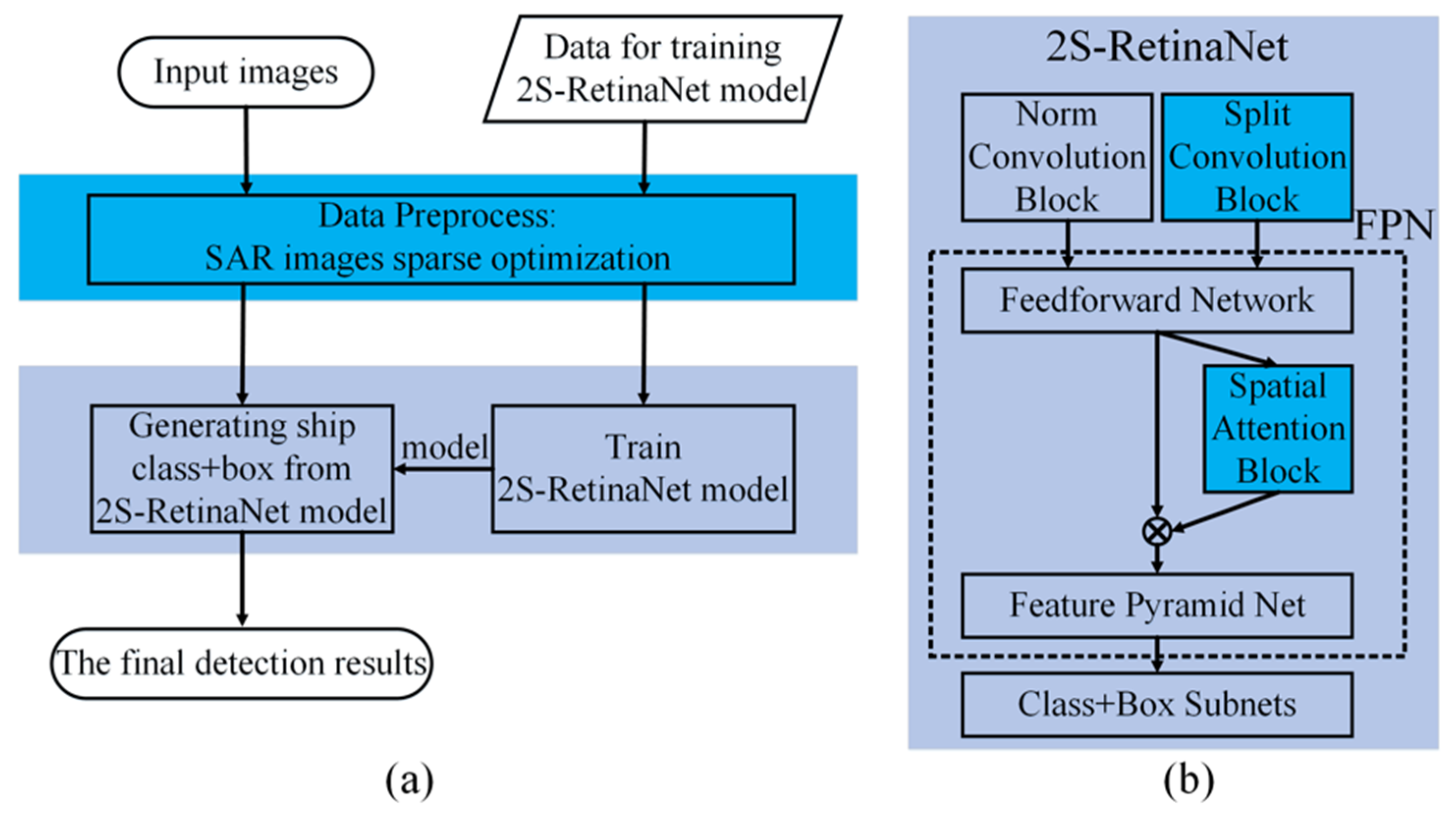
2. Materials and Methods

The overall scheme of the proposed method and the network architecture of 2S-RetinaNet (Split Convolution and Spatial Attention Blocks-RetinaNet) are shown in Figure 1. As shown in Figure 1a, before sending the SAR images into the network, we perform the sparse optimization on the input SAR images to achieve clutter and sidelobe suppression, and improve the signal to clutter ratio of the image. Due to the SAR image quality in the dataset, the sparse optimization is carried at muti-levels. On the basis of RetinaNet, two self-designed modules, namely SCB and SAB are embedded. The locations of these two modules in the overall network are shown in Figure 1b. SCB divides the input SAR images into smaller parts to improve the attention to small and densely clustered ships. And SAB optimizes the feature maps of the FPN feedforward network, strengthens the attention to the target area, and reduces the loss of spatial information during the feature maps transfer between the feedforward network and the feature pyramid net. After that, the box and class regression subnets will predict the target position and classification with the multi-layer feature maps extracted by FPN. The addition of SCB and SAB will not change the convergence of RetinaNet. At the same time, the increased running time is acceptable after the two lightweight modules embedded.

In addition, based on the distribution of the bounding box in the dataset, we re-design the structure of RetinaNet and the size of the anchor of each layer in FPN. In the following sections, the SAR image sparse optimization, the background on RetinaNet and the three improvements on RetineNet: multi-scale anchor design, SCB and SAB, are presented.

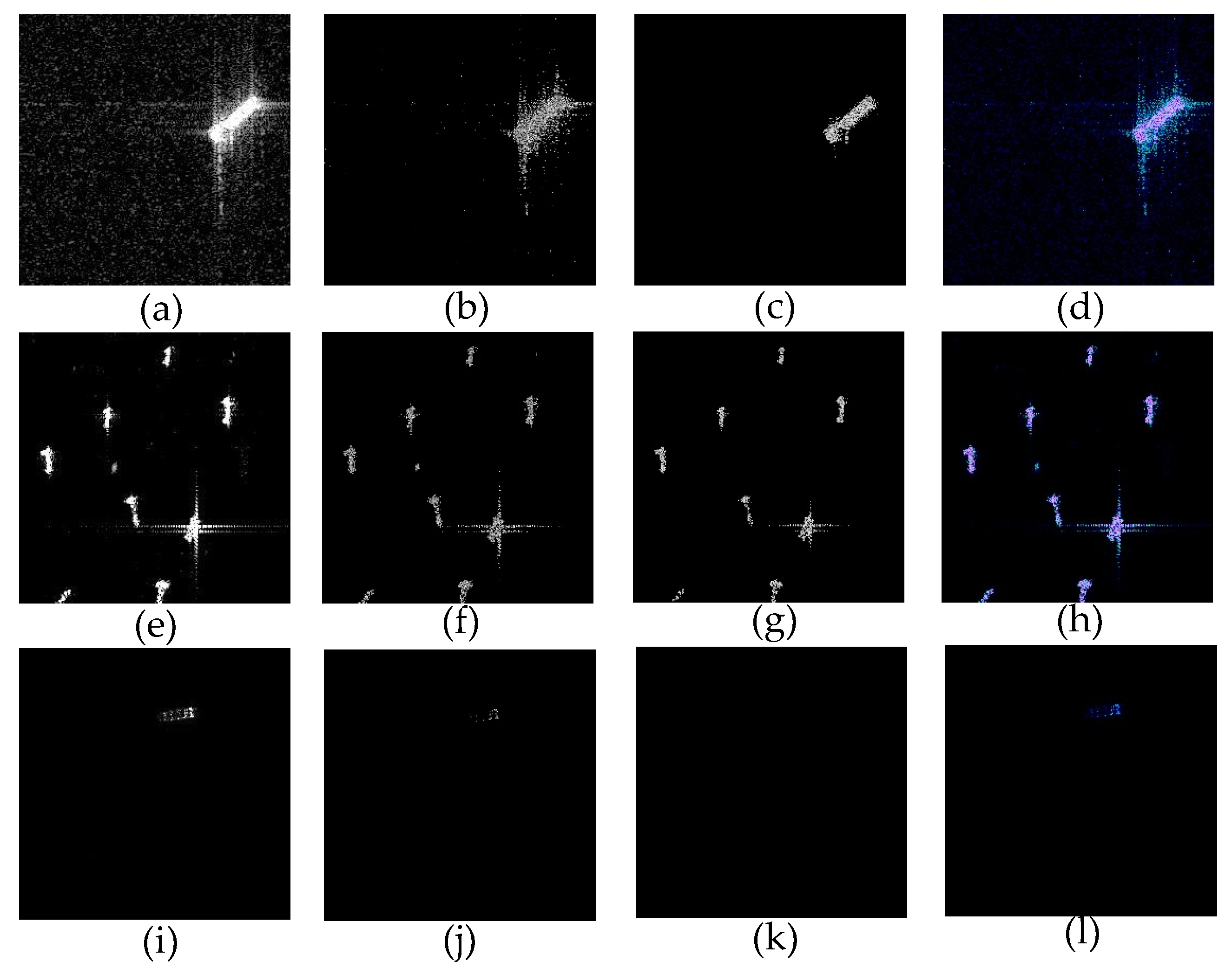
2.1. Data Preprocess: SAR Image Sparse Optimization

For space-borne SAR systems, the radar receives echo signals from the ground, including ground-based stationary clutter and moving target signals. Since the spectrum of the clutter is wide and the energy of the clutter is much stronger than the energy of the target, we need to suppress the clutters to improve the target detection ability. In the multi-targets SAR images, the high-level sidelobes of the strong scattering point will mask the low-level main lobe of the adjacent weak scatter target, resulting in the missed detection of the weak targets. Due to the metal materials and the superstructure of the ship, ships have strong backscatters. Generally, the metallic ship cockpits produce bright lines along the range or the azimuth directions which are caused by the sidelobe effect. These bright lines will reshape the ship appearances in the SAR images and disturb the detection process.

In this paper, we perform sparse optimization via an iterative thresholding algorithm to enhance the features of the SAR image at first. Compared with the traditional SAR feature enhancement methods, it can achieve the performance improvement in clutter, sidelobe and azimuth ambiguity suppression, with additional advantage of lower computational complexity and memory consumption. As for a SAR image obtained by radar system, it can be decomposed as follows:

$$Y=X+N$$

(1)

where $X$ is the considered scene. $N$ is a complex matrix of the same size as $X$, which denotes the difference between reconstructed image and the real scene, and includes noise, sidelobe, clutter, azimuth ambiguity and so on. Considering the sparsity of SAR images, we can recover the considered scene by solving the following optimization problem:

$$\widehat{X}=\underset{X}{\min }\left\{{\Vert Y-X\Vert }_F^2+\lambda {\Vert X\Vert }_q^q\right\}$$

(2)

Here, we take $L_q$ regularization-based synthetic aperture radar image feature enhancement, and $q\in (0,1]$. Where $\widehat{X}$ is the $L_q$ regularization-based reconstructed scene,$\lambda$ is the regularization parameter and ${\Vert •\Vert }_F^{}$ is the Fresenius norm of a matrix. An iterative thresholding algorithm is often used to solve the optimization problem [40]. When $q=1$, the detailed approximated sequence of the solution can be represented as:

$$X^{(i+1)}=f(X^{(i)}+\mu (Y-X^{(i)}),\mu \lambda )$$

(3)

where $X^{(i)}$ is the reconstruction scene of the $i$th iteration and $f(.)$ is the thresholding operator. $\mu$ controls the convergence speed of the iterative algorithm. The regularization parameter $\lambda$ controls the reconstructed precision and the estimated scene sparsity. $\lambda$ is updated after each iteration:

$${\lambda }^{(i)}={\left|X^{(i)}+\mu \Delta X^{(i)}\right|}_{K+1}/\mu$$

(4)

where $\Delta X^{(i)}$ represents the difference between the reconstruction scene of the current iteration ($X^{(i)}$) and the original image ($Y$). And ${\left|X^{(i)}+\mu \Delta X^{(i)}\right|}_{K+1}$ denotes the (K+1)st largest amplitude element of the image, where K is a parameter denoting the scene sparsity, which can be obtained by calculating the zero norm of the reconstruction scene ($X^{(i)}$):

$$K\stackrel{\Delta }{=}{\Vert X^{(i)}\Vert }_0/M$$

(5)

where M is the number of the pixels of $X$. $K$ and $\lambda$ are updated after each iteration, and the sparse reconstruction scene of the current iteration is:

$$X^{(i+1)}=\mathrm{sgn}(X^{(i)}+\mu \Delta X^{(i)})·\max (\left|X^{(i)}+\mu \Delta X^{(i)}\right|-\mu \lambda ,0)$$

(6)

After multiple iterations, the signal values with lower amplitudes in the input scene will be set to zero to achieve clutter and sidelobe suppression. The number of the iteration has a great impact on the sparsity and precision of the reconstruction scene. Less iterations will retain more details in the original image, but at the same time the clutter and sidelobe suppression are not thorough enough. If the number of the iteration is set too high, the clutter and sidelobe will be better removed, but the details of the input image may be lost. As for the input SAR images with different quality, here we use the sparse reconstructed images under different iterations as the input of the network. In Figure 2, three original SAR images are shown respectively, with iterations of 50 and 80, and three-channel RGB images that are fused with the original images and two sparse reconstruction images.

As shown in Figure 2a–c, clutters and sidelobes in the SAR images are suppressed in the two dimensions of distance and azimuth, and the target becomes clearer with the increase of iterations. When the number of iterations is high, the non-target spots in the SAR image will be removed, which will reduce false alarms during the detection process. However, too many iterations will also cause the loss of the SAR target details. As shown in Figure 2j,k, some or all of the target features in SAR images are lost. SAR images with different quality need sparse optimization with different iterations. Therefore, we choose the original image, 50 and 80 iterations as the input of the network. As can be seen from Figure 2d,h,l, such a method enables the SAR images with different quality to be clutters and sidelobes suppressed without losing the original target features.

Deep learning networks are designed based on the optical images, and the input image has three input channels of RGB. For SAR grayscale images, there is only one input channel. In order to widely apply deep learning networks to SAR images, the common measure is to adopt the same grayscale image for all the three input channels. As a result, the features learned on these three channels will be overlapped. In this paper, the SAR original image and the image enhancement under two levels are taken as input, which enriches the characteristics of the SAR images and enables the network to learn more.

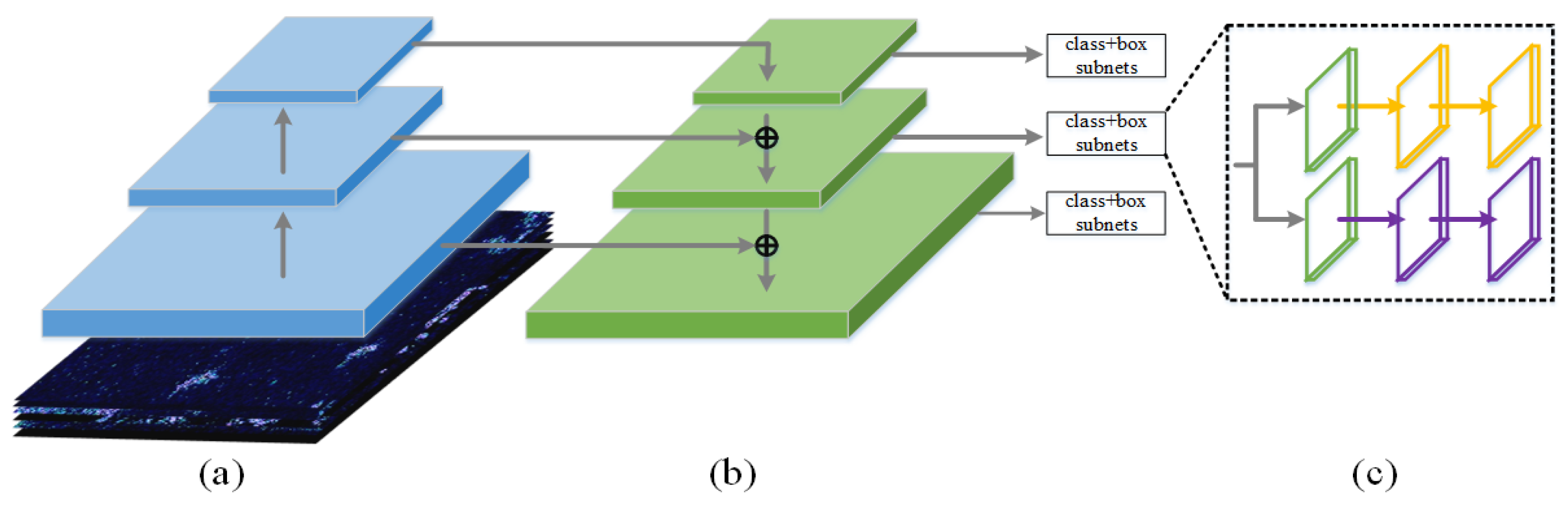
2.2. Background on RetinaNet

RetinaNet is a one-stage detector and mainly consists of a backbone network and two sub-networks. The network structure is shown in Figure 3. Figure 3a shows the bottom-up pathway for feature extraction, (b) shows the top-down pathway for feature fusion, (a) and (b) together form the backbone network FPN and (c) is the two subnetworks. FPN acts as a feature extractor with the consideration of the low-level high-resolution and high-level low-resolution semantic meaning. FPN mainly solves the multi-scale problem in object detection. By simply changing the network connection, the detection performance of small objects is greatly improved without substantially increasing of the calculation. The feedforward network of FPN usually consists of CNNs, such as VGG [27], Inception [28,29,30], ResNet [41,42] and DenseNet [43]. The two subnets are composed of the fully convolution network (FCN) [44]. One subnet is used for predicting the bounding box of the targets, and the other is used to predict the classification of the targets. Except for the final convolution layer, the design of the box regression subnet is identical to the classification subnet. The two subnets share a common structure but use separate parameters.

In order to solve the problem of class imbalance in object detection, RetinaNet adopts focal loss as the loss function. Focal loss is an improved cross entropy loss, which multiplies an exponential term to weaken the contribution of easy examples. In Section 2.2.1 and Section 2.2.2, we will introduce FPN and Focal loss in detail.

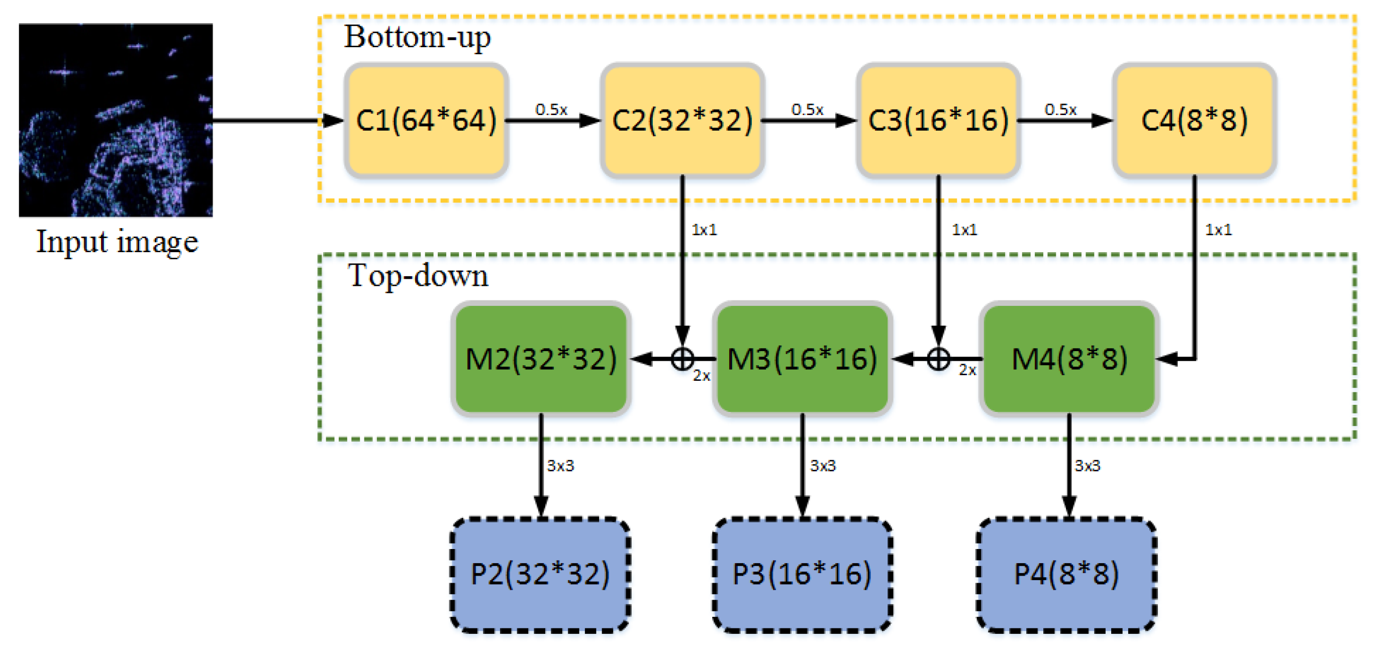
2.2.1. FPN (Feature Pyramid Network)

As shown in Figure 3, there are two pathways in FPN. The bottom-up pathway usually consists of CNNs to extract hierarchical features. The spatial resolution decreases from bottom to top, and semantic information in the feature maps increases as the network hierarchy is getting deeper.

The top-down pathway hallucinates higher resolution features by up-sampling spatially coarser, but semantically stronger, feature maps from higher pyramid levels. Then, these features are enhanced with the features from bottom-top pathway via lateral connections. The lateral connection merges the feature maps from the bottom-top and top-down pathways. The feature maps from the bottom-up pathway are of lower-level semantics, but more accurately localized as it is subsampled fewer times. As a result, the feature maps used for prediction features have different resolutions and semantic meanings. Such an operation only adds additional cross-layer connections on the basis of the original network, it hardly consumes extra time and computation.

To see more clearly, the architecture of FPN used in our method is presented in Figure 4. As shown in Figure 4, the input images used in this paper has a size of 256 × 256. After four convolution modules, the feature maps with a size of 32 × 32, 16 × 16, 8 × 8 {C2, C3, C4} are obtained, respectively. The skipped connections apply 1 × 1 convolution to reduce the channels of {C2, C3, C4} to 256. After that, {M2, M3, M4} are obtained by combining the up-sampling feature maps with the corresponding bottom-up feature maps. Finally, a 3 × 3 convolution is used to obtain the feature maps for classification and bounding box regression. The final feature maps set is {P2, P3, P4}, with the same length and width as {C2, C3, C4}, respectively.

2.2.2. Focal Loss

As a one-stage object detector, RetinaNet adopts the focal loss to handle the problem of class imbalance and unequal contribution of hard and easy examples. Classic one-stage object detection methods evaluate 10⁴–10⁵ candidate locations per image, but only a few locations contain targets, which leads to a large class imbalance during the training process. The training loss is dominated by the majority of the negative samples, and the key information provided by a few positive samples cannot play a role in the commonly used training loss. So a loss that can provide correct guidance for model training cannot be obtained. The class imbalance will result in the inefficient training, and the easy negatives can overwhelm training and degenerate the model.

The focal loss reshapes the loss function to down-weight easy examples and focus training on hard negatives, which adds a modulating factor to the cross entropy loss. The focal loss is defined in Equation (7):

$$\mathrm{FL}(p_t)=-{\alpha }_t{(1-p_t)}^{\gamma }\log (p_t)$$

(7)

In Equation (7) ${\alpha }_t,\gamma$ are the two hypermeters which are used for moderating the weights between easy and hard examples. Where the tunable focusing parameter $\gamma \ge 0$. When $\gamma =0$, the focal loss is equivalent to the cross loss. For notational convenience, we define $p_t$ in Equation (8):

$$p_t=\{\begin{array}{c}p\\ 1-p\end{array}\begin{array}{c}\\ \end{array}\begin{array}{c}if\hspace{1em}y=1\\ otherwise\end{array}$$

(8)

where $p$ is the probability estimated by the model and $y=1$ represents the ground-truth.

Once the weight ${\alpha }_t{(1-p_t)}^{\gamma }$ is multiplied, the training loss contributed by large negative categories (such as background) drastically reduces, and loss contributed by small positive categories reduces a little. Although the overall training loss reduces, the category with less amount in the training process occupies more proportion of the training loss, which is paid more attention by the network.

2.3. The Improvements on RetinaNet

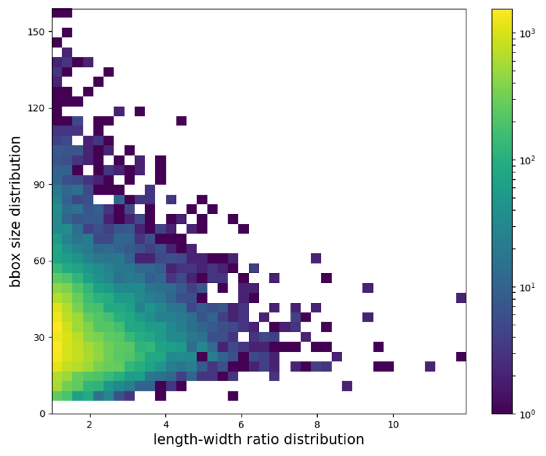
2.3.1. Multi-Scale Anchor Design

Target detection methods based on deep learning usually generate the predicted region proposals of the target at each position on the feature map. In order to reduce the number of predicted proposals, several fixed region proposals are given, which are called anchors. Anchor converts the object detection problem into the regression problem between each proposal and its assigned object box [45]. By this way, the problem of high detection miss rate caused by multiple objects in the same area can be solved. The size of anchor is critical to network performance. In the deeper layers of the feedforward network, the feature maps have more semantics, so that the anchor size is set larger to detect larger objects. The small anchor on the feature maps obtained by the shallow network is used to detect small objects.

The SAR ship detection dataset used in this paper is of multi-resolution, and different types of ships have different sizes, so that the ship in the chips has various sizes. In addition, the SAR images are affected by the imaging mode, and the geometric deformation caused by the incidence angle will also result in the change of the ship shape in chips. Here, we use the multi-layer feature maps for ship detection, and we need to design the multiple anchor sizes for the SAR ship detection dataset. We count the distribution of the bounding box size in the dataset and take into account the comprehensive size and the aspect ratio of the bounding box. Taking $\sqrt{l_{bbox}\times s_{bbox}}$ as the horizontal axis and $\raisebox{1ex}{$l_{bbox}$}\!\left/ \!\raisebox{-1ex}{$s_{bbox}$}\right.$ as the vertical axis, we locate each bounding box in a two-dimensional coordinate graph, so as to have a comprehensive understanding of the distribution of the bounding box size. Here, $l_{bbox}$ and $s_{bbox}$ are the lengths of the long side and the short side of each bounding box. The result is shown in Figure 5.

In Figure 5, the color bar on the right represents the number of bounding boxes, and the number increases from blue to yellow. As shown in Figure 5, the sizes of most bounding boxes are regular with the comprehensive size of 30^2 and the aspect ratio between 1 and 2. Based on this, we re-design the size of the anchor. As mentioned in Section 2.1, in order to avoid high computational complexity, the feature maps {P2, P3, P4} are used for prediction. The anchors of deeper layers cover a huge area with respect to the network’s input image, which will only overlap a few huge objects. The size of the input SAR image is 256 × 256 and the anchors have the base areas of 16^2, 32^2, 64^2, respectively. At each pyramid level, the anchors have three aspect ratios {1:2, 1:1, 2:1}. For dense scale coverage, at each level we add anchors of sizes {0.4, 0.8, 1.2} of the original set of three aspect ratio anchors. In total, there are nine anchors per level and across levels they cover the scale range of 6.4–76.8 pixels with respect to the network’s input image. These anchors can cover most bounding boxes in the dataset, and will not result in a huge model with too many anchors.

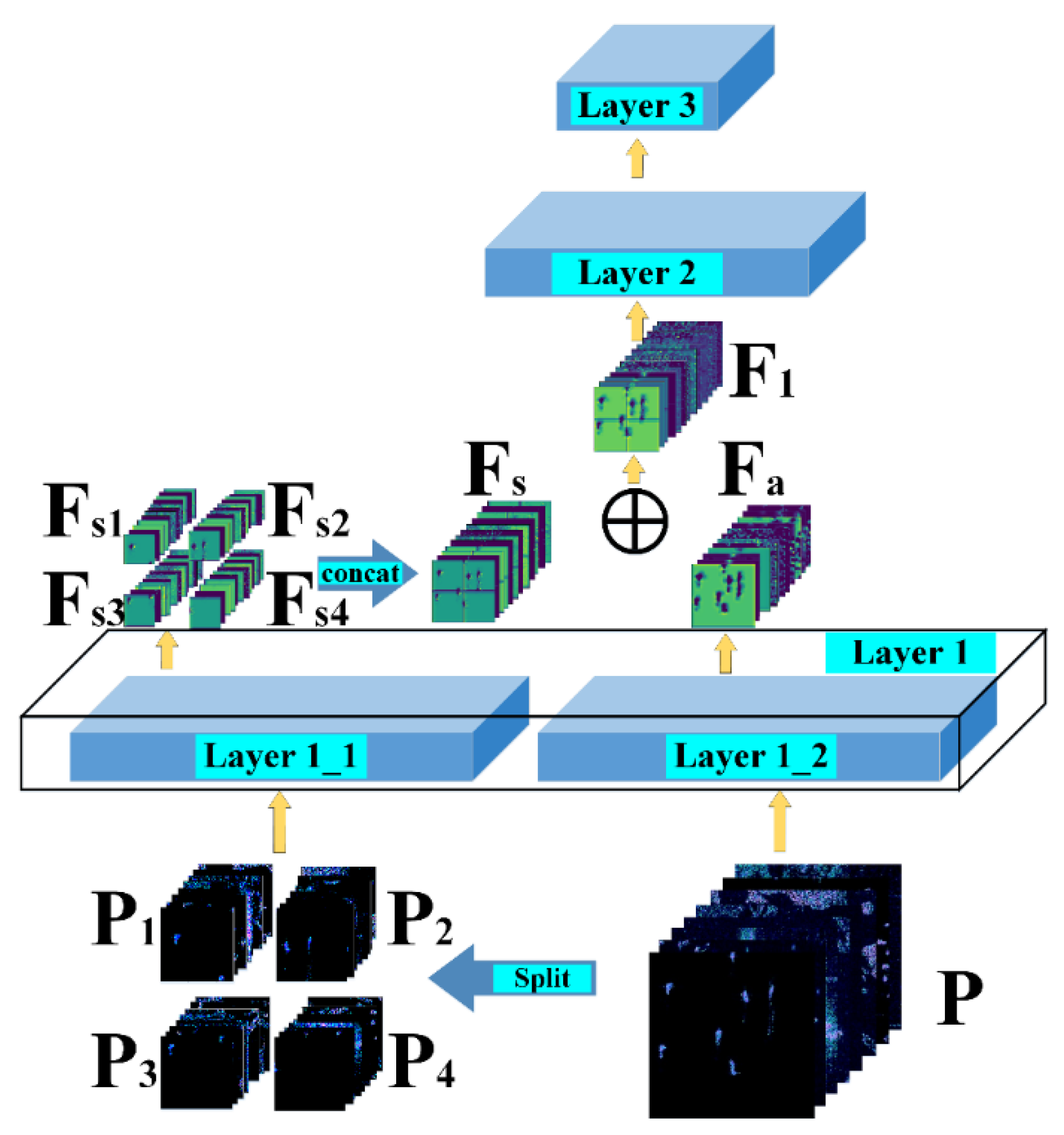
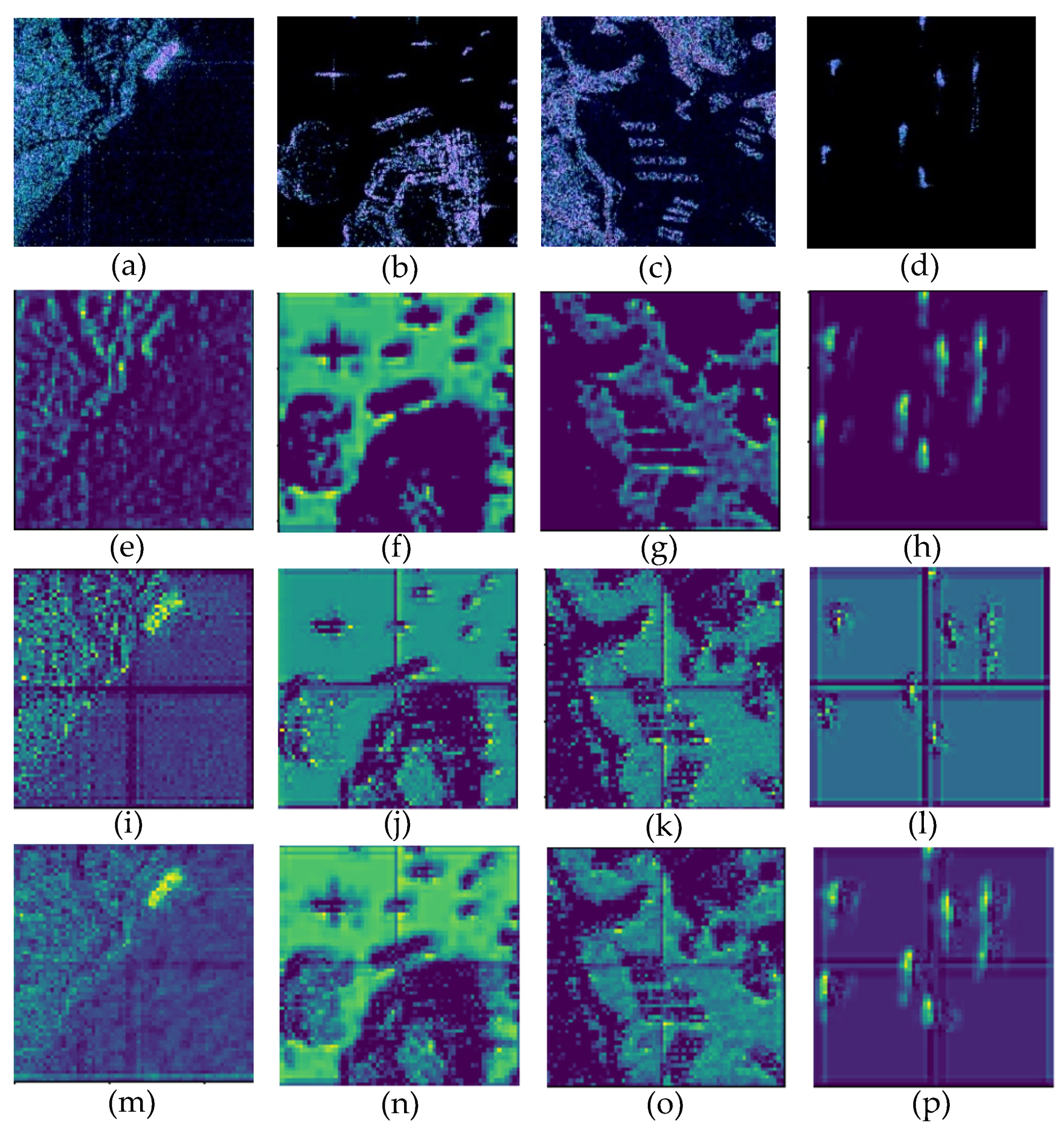
2.3.2. Split Convolution Block (SCB)

In order to improve the feature extraction performance of small targets, we propose a new convolution block, namely, split convolution block (SCB); that is, the original input image is divided into several sub-images of the same size and used as the input of the network. In order to avoid the discontinuity of target features caused by some targets at the edge of clipping, here we still keep a normal convolution block and take the complete SAR image as input. At the same time, the overall characteristics of the input image are also what we need to pay attention to. After the first convolution module, the feature maps corresponding to the sub-images are spliced and fused with the feature maps of normal convolution. Through the combination of SCB and normal convolution, the feature extraction of target is obtained in a finer granularity so as to retain more detailed features and improve the detection accuracy of small targets.

The inspiring idea of this paper is the global precedence in visual perception [46,47]. That is to say, most people are more sensitive to the overall features than the local details, which makes them neglect the key details when they pay attention to the target, especially the small targets. The operation object of convolution is the whole input image with convolution kernels of fixed sizes. When the region of interest is large, it is difficult for the network to obtain complete details of the target with limited convolution parameters, resulting in the loss of information. In order to reduce such an information loss caused by the global precedence and improve the network’s attention to SAR image details, SCB splits the large image into several small ones as the inputs of the network. The proportion of the target area in the small ones will be larger and the details will be more prominent. By processing the inputs of small size, the feature extraction of the target will be much easier. In this paper, we cut the input image into four sub-images of the same size, namely, the cutting positions are the middle of the distance and azimuth dimensions. The bottom-up pathway of FPN with SCB is shown in Figure 6.

As shown in Figure 6, given the input SAR images $P\in {ℝ}^{C\times H\times W}$, we cut them in half of W/H and obtain four reduced sub-images $P_i\in {ℝ}^{C\times \frac{H}{2}\times \frac{W}{2}}(i=1,2,3,4)$. Such a process can be summarized as:

$$P_i=split{(split{(P)}_{\frac{H}{2}})}_{\frac{W}{2}}(i=1,2,3,4)$$

(9)

After that, we input $P$ and $P_i(i=1,2,3,4)$ into the first convolution module of the network and obtain feature maps $F_a\in {ℝ}^{c\times h\times w}$ and $F_{si}\in {ℝ}^{c\times \frac{h}{2}\times \frac{w}{2}}(i=1,2,3,4)$, respectively. The relative position of $F_{si}(i=1,2,3,4)$ is shown in Figure 6. After obtaining the four groups of feature maps of SCB, we first concatenate them at the corresponding channel and spatial position to obtain the feature maps $F_s\in {ℝ}^{c\times h\times w}$ with the same size as the feature maps $F_a\in {ℝ}^{c\times h\times w}$ of normal convolution. The splicing process can be expressed as Equation (10).

$$F_s=concat(concat{(F_{s1},F_{s2})}_{\frac{w}{2}}),concat{(F_{s3},F_{s4})}_{\frac{w}{2}}){)}_{\frac{h}{2}}$$

(10)

where $concat{(•)}_{\frac{w}{2}},concat{(•)}_{\frac{h}{2}}$ denotes concatenating at the position of $\frac{w}{2},\frac{h}{2}$. After that, $F_a$ and $F_s$ are added on the corresponding channel, generating the optimized feature maps $F_1\in {ℝ}^{c\times h\times w}$.

$$F_1{=F}_a\oplus F_s$$

(11)

where $\oplus$ denotes adding element-by-element at the corresponding convolution channels.

The optimized feature maps $F_1\in {ℝ}^{c\times h\times w}$ are used as the input of the next convolution module. In this way, SAR image feature extraction is enhanced.

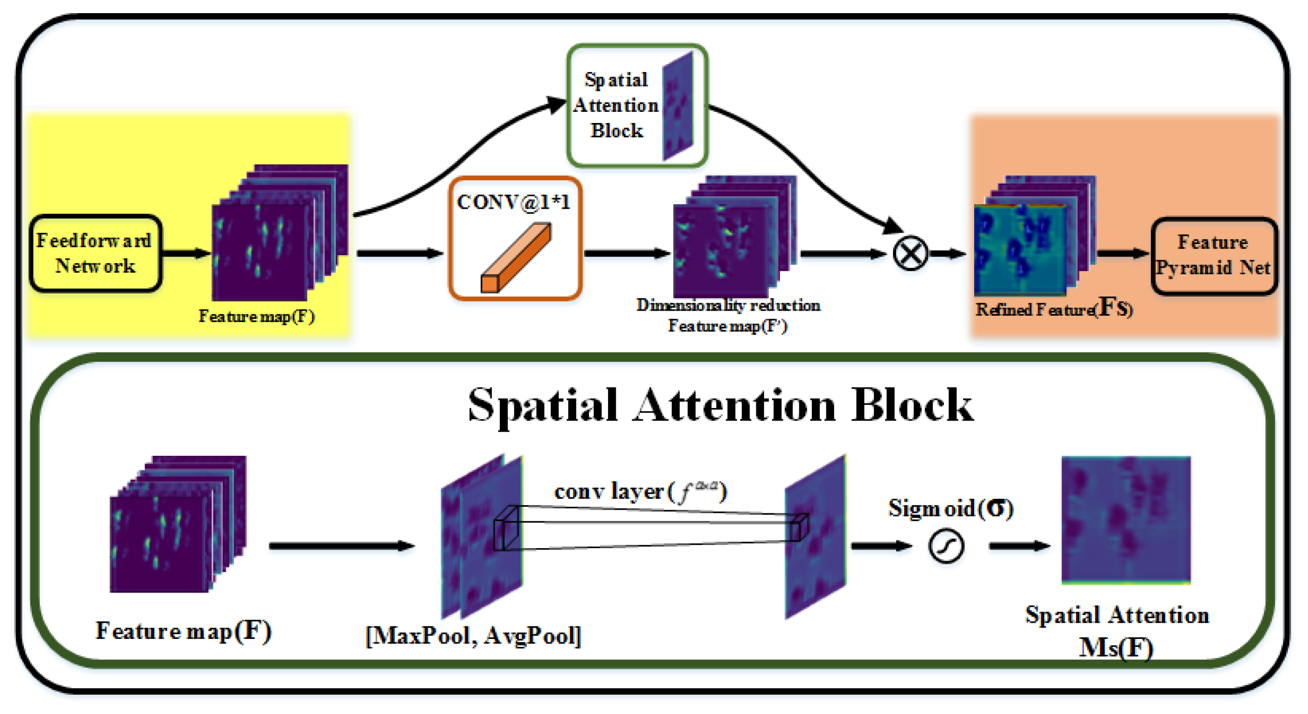
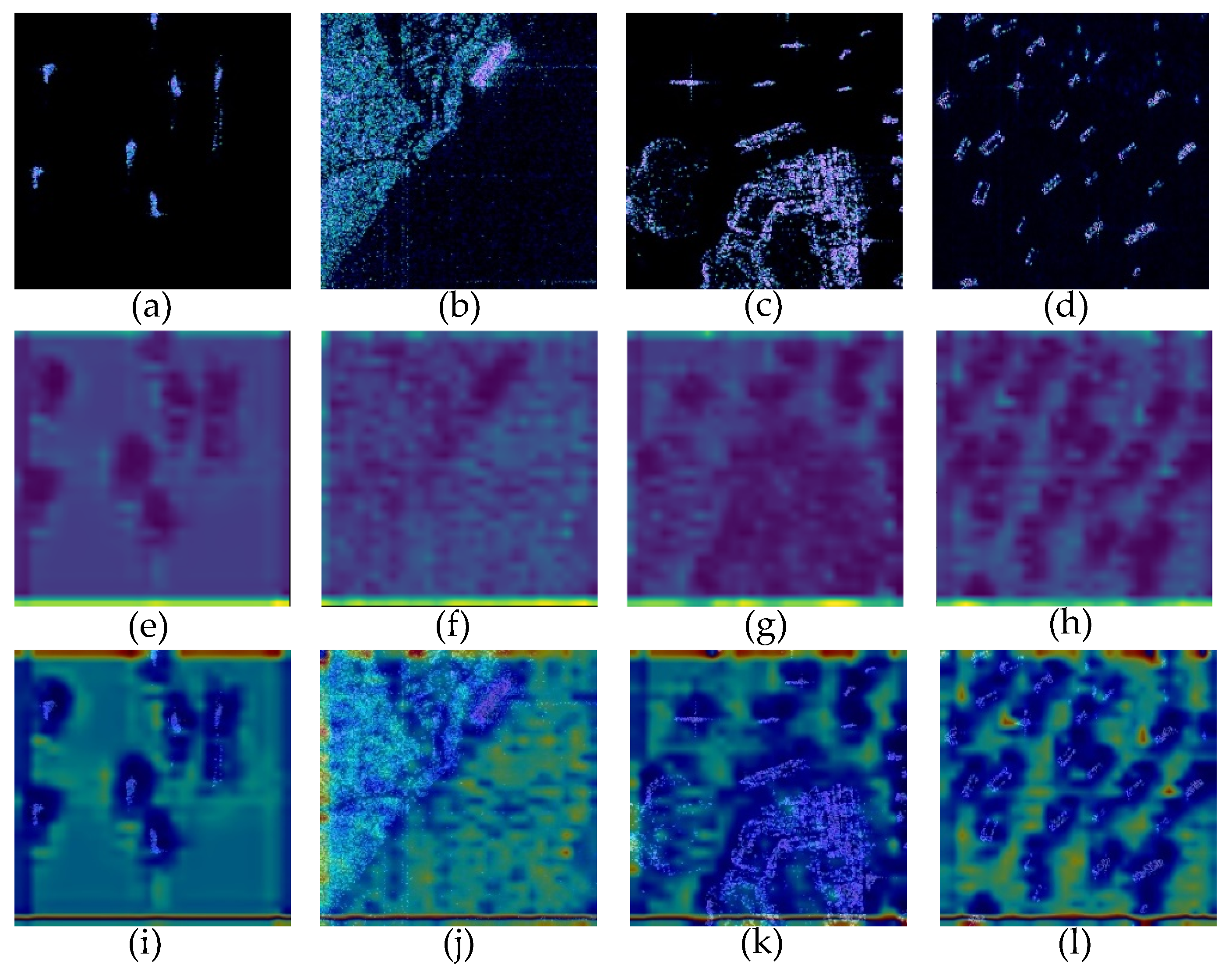
2.3.3. Spatial Attention Block (SAB)

We embed SAB in FPN to optimize the performance of the network from the perspective of the attention mechanism. SAB efficiently helps the information flow within the network by learning which information to emphasize or suppress. The location of SAB in FPN is shown in Figure 1. As shown in Figure 4, in FPN, when the feedforward network (bottom-up pathway) and the feature pyramid net (top-down pathway) are connected, 1 × 1 convolution is adopted to reduce the feature map channels to a fixed number 256. Through such a design, the feedforward network and the other parts of FPN are separated so that the change of the feedforward network structure will not affect the feature pyramid net, box and class subnets. In addition, the network will be more compact with the help of dimensionality reduction with 1 × 1 convolution. FPN realizes the target detection based on the feature maps of multiple layers and too many feature maps will make the network architecture too large and take a long time to train.

Basically, 1 × 1 convolution has two main functions. One is to realize the cross-channel interaction and information integration of feature maps in different channels, so as to improve the expression ability of the network. The second is to reduce or increase the number of feature map channels, so as to increase the nonlinearity of CNNs and facilitate the optimization of network structure. The 1 × 1 convolution simply maps the values at the same location of all channels to one value, without considering the spatial information along the W/H dimension of the feature maps. For the purpose of enlarging the receptive field of 1 × 1 convolution, Inception adds 3 × 3 and 5 × 5 convolution in parallel to obtain the receptive field of different sizes and extract the features on different scale. However, the increase of the network width results in the degradation of the network computational performance. In order not to significantly increase the computational complexity, we embed SAB in FPN to enhance the spatial information on the feature maps [48,49]. SAB infers a 2D spatial attention map and refines the feature maps of the feedforward network. By multiplying the spatial attention map and the feature maps with channel reduced by 1 × 1 convolution, the feature maps refined on spatial-wise will obtained. The location and specific implementation process of SAB are shown in Figure 7.

Here, we take the feature maps output by the feedforward network $F_1\in {ℝ}^{c\times h\times w}$ as an example to introduce the whole implementation process in detail. Firstly, the dimensionality reduced feature map $F_1{}^{\prime }\in {ℝ}^{c^{\prime }\times h\times w}$ is obtained by the convolution with 1 × 1 kernel.

$$F_1{}^{\prime }=f^{1\times 1}(F_1)$$

(12)

where $f^{1\times 1}$ denotes the convolution with the kernel of size $1\times 1$.

In addition to 1 × 1 convolution, we also input $F_1$ into SAB. The specific approach is to make global average pooling and global max-pooling along the channel axis of $F_1$ so as to obtain the pooling result with a size of $h\times w$, and a channel of 2. After that, we concentrate on the pooling result and generate an efficient feature descriptor. As shown in Figure 7, on the concatenated feature descriptor, a $a\times a$ kernel is applied to generating a spatial attention map $M_s\left(F_1\right)\in {ℝ}^{1\times h\times w}$ which encodes where to emphasize or suppress. The process of getting $M_s\left(F_1\right)$ can be summarized as follows:

$$M_s\left(F_1\right)=\sigma (f^{a\times a}(\left[\mathrm{Avgpool}(F_1);\mathrm{Maxpool}(F_1)\right]))=\sigma (f^{a\times a}(\left[F_1{}_{avg}^s;F_1{}_{\max }^s\right]))$$

(13)

where $\sigma$ denotes the sigmoid function and $f^{a\times a}$ denotes the convolution with a kernel of size $a\times a$. We take the kernel size of 3 × 3 in SAB of our model.

By multiplying the spatial attention map $M_s\left(F_1\right)$ and dimensionality reduced feature maps $F_1{}^{\prime }$, the output feature maps refined on spatial-wise $F_{1s}\in {ℝ}^{c^{\prime }\times h\times w}$ can be obtained:

$$F_{1s}=M_s\left(F_{{}_1}\right)\otimes F_1{}^{\prime }$$

(14)

where $\otimes$ denotes element-wise multiplication.

By this way, we transfer the feature maps with enhanced spatial features to the feature pyramid net for feature fusion. One can seamlessly integrate SAB in FPN with a slight modification and SAB will not change the convergence of baseline model. With the lightweight architecture of SAB, the increased running time of SAB can be neglected which is verified in the experiments section.

3. Results and Discussions

3.1. Configuration

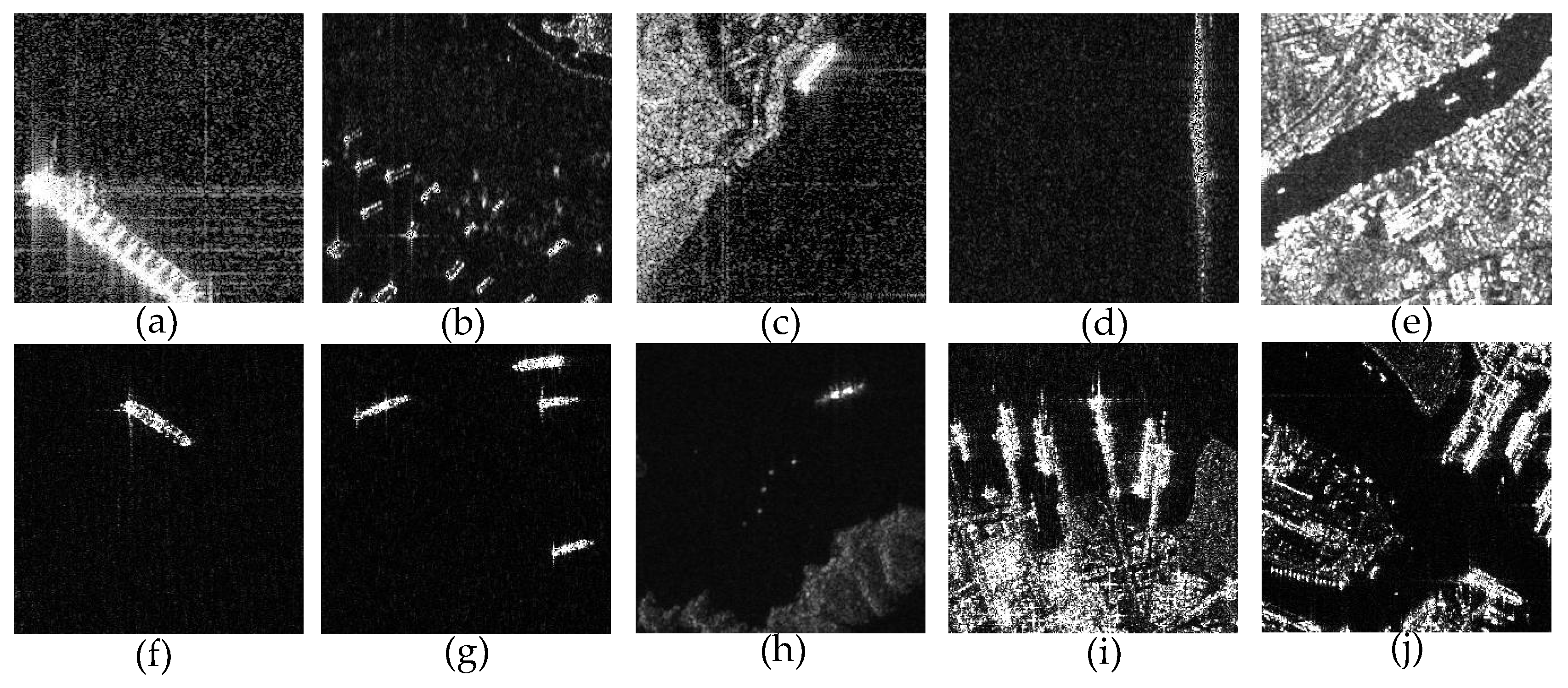
3.1.1. Dataset Description

The dataset used in this paper is a SAR dataset for ship detection published by the Digital Earth Laboratory of the Aerospace Information Research Institute, Chinese Academy of Sciences [50]. There are 102 GaoFen-3 images and 108 Sentinel-1 images that are used to constructed the dataset. As for GaoFen-3, the resolution of these images involves 3 m, 5 m, 8 m and 10 m with Strip-Map (UFS), Fine Strip-Map 1 (FSI), Full Polarization 1 (QPSI), Full Polarization 2(QPSII) and Fine Strip-Map 2 (FSII) imaging mode, respectively. The Sentinel-1 imaging modes are S3 Strip-Map (SM), S6 SM and IW-mode. The details of these images are shown in

Table 1. The quantitive detection results Detailed information for original SAR imagery.

Sensor	Imaging Mode	Resolution Rg. × Az.(m)	Swath (km)	Incident Angle (°)	Polarization	Number of Images
GF-3	UFS	3 × 3	30	20~50	Single	12
GF-3	FS1	5 × 5	50	19~50	Dual	10
GF-3	QPSΙ	8 × 8	30	20~41	Full	5
GF-3	FSΙ	10 × 10	100	19~50	Dual	15
GF-3	QPSΙΙ	25 × 25	40	20~38	Full	5
Sentinel-1	SM	1.7 × 4.3 to 3.6 × 4.9	80	20~45	Dual	49
Sentinel-1	IW	20 × 22	250	29~46	Dual	10

, including imaging mode, resolution, incidence angle and polarization.

Based on these preprocessed SAR images, sliding windows are used to acquire ship chips of 256 × 256 pixels in size. In order to enrich the backgrounds of these chips, adjacent sliding windows have overlapping of 128 pixels in both horizontal and vertical directions. Currently, there are 43,819 ship chips in this dataset and each ship chip is labeled by SAR experts.

From Figure 8, we can see that the dataset has the following three characteristics. First, there are multi-size SAR ships in these chips, and the size conversion range is large. Second, there are complex backgrounds in the ship chips. Some of ships are on the open sea, some in the port. Third, the distribution of these ships has many forms, including independent cruising and fleet sailing. All of these have brought difficulties to ship detection, and put forward higher requirements for the performance of ship detection. In the experiment, we divide the training and testing set randomly according to the rate of 7:3. A total of 30,673 ship chips are used for training and 13,146 ship chips are used for testing.

3.1.2. Evaluation Metrics

In order to make a quantitative evaluation of the experimental results, we adopt four widely used criteria, namely, precision, recall, mAP (mean Average Precision) and F1 score. The precision measures the fraction of detections that are true positives and the recall measures the fraction of positives over the number of ground-truths, given by [51].

$$\{\begin{array}{c}precison=\frac{N_{TP}}{N_{TP}{+N}_{FP}}\\ recall=\frac{N_{TP}}{N_{TP}{+N}_{FN}}\end{array}$$

(15)

where $N_{TP}$, $N_{FP}$ and $N_{NF}$ represent the number of true positives, the number of false positives and the number of false negatives.

As for object detection, a higher precision and a higher recall are both expected. Whereas, in fact, precision and recall are a pair of contradictory indicators. It means that a higher precision will result in a lower recall and a higher recall will result in a lower precision. F1 score is a commonly used criteria in object detection, which can comprehensively evaluate precision and recall. A higher F1 score means a more ideal comprehensive detection performance [52]. F1 score is defined based on the harmonic average of precision and recall:

$$F1=2\times \frac{precison\times recall}{precison+recall}$$

(16)

Precision, recall and F1 score are all calculated based on the single point threshold. mAP can solve the limitations of single point threshold and get an indicator that reflects the global performance. mAP is obtained by the integral of the precision over the interval from recall = 0 to recall = 1, that is, the area under the precision-recall (PR) curve [53].

$$mAP={\displaystyle {\int }_0^{1}P\left(R\right)dR}$$

(17)

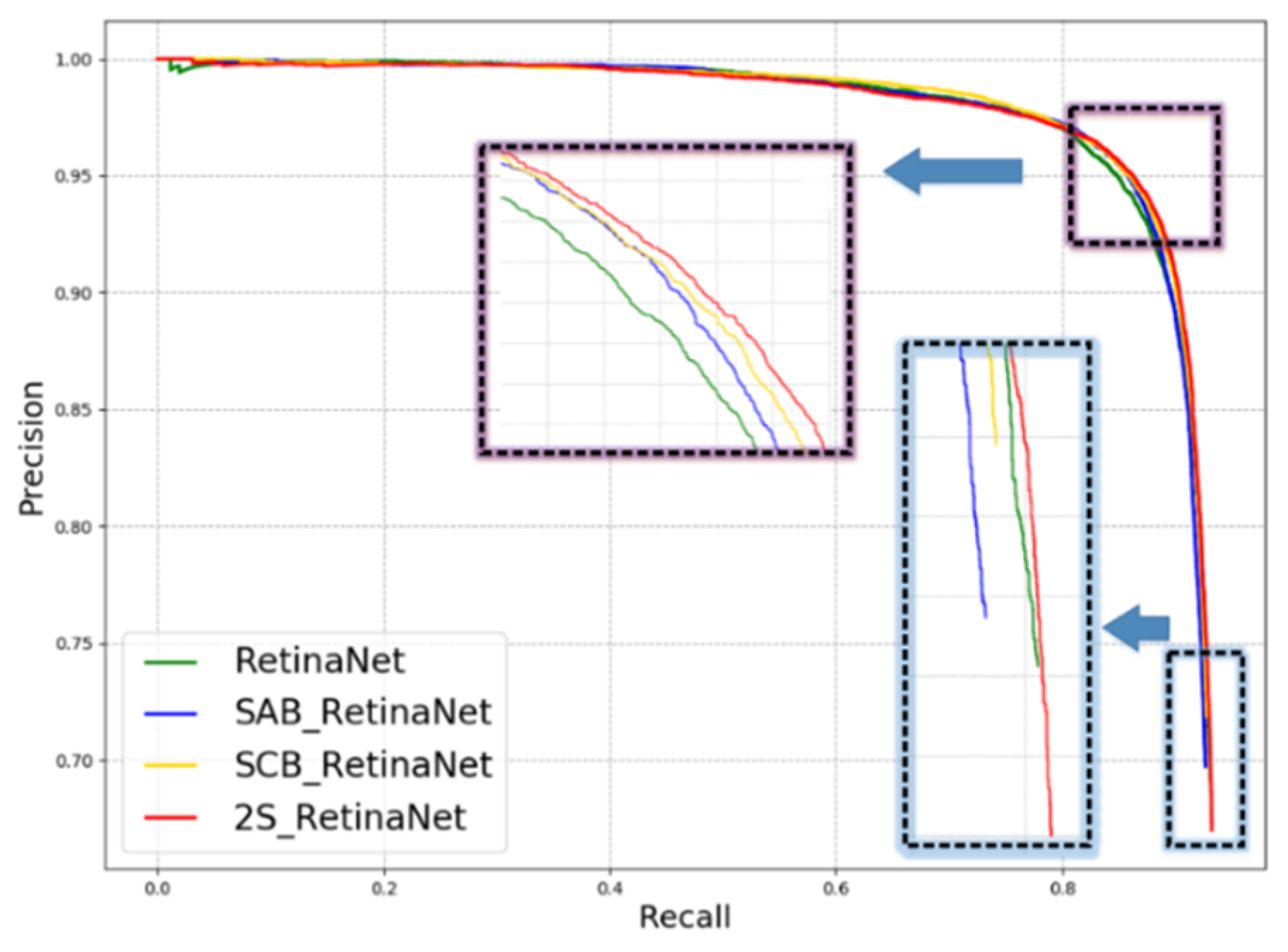
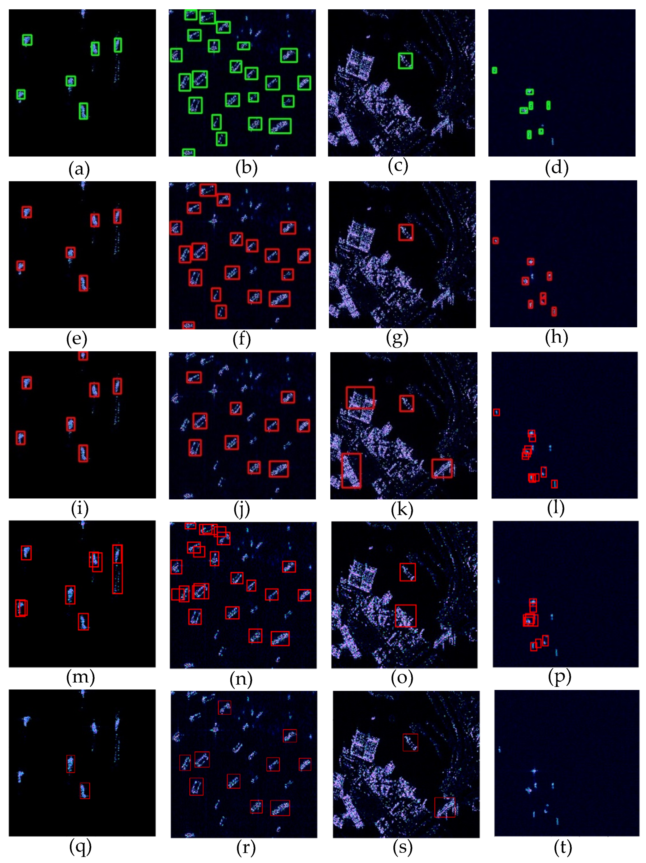
3.2. Experiment Results

The baseline model used in this paper is RetinaNet. In order to verify the effectiveness of the proposed SCB and SAB, we conduct the following comparison experiments under four conditions: RetinaNet, SAB-RetinaNet (RetinaNet embedded with SAB), SCB-RetinaNet (RetinaNet embedded with SCB), 2S-RetinaNet (RetinaNet embedded with SAB and SCB). The bottom-up pathway of FPN under each condition consists of the same ResNet. At the beginning of network training, we use the parameters pre-trained on ImageNet to initialize the network and fine-tune the system on this bias [54]. We train 100 iterations under each experiment condition, and all the other training parameters are consistent. During the training and testing process, the IoU (Intersection over Union) value adopts a uniform 0.5, that is, the ratio of the intersection and the union between the candidate bounding box and the ground truth should be greater than or equal to 0.5. The IoU value will affect the precision and recall of object detection, especially the recall. A high IoU value will lead to a low recall and 0.5 is the common used value for object detection. The PR curves of the four experiments are plotted in Figure 9. The x and y axes are the recall and precision.

On the PR curves, if one algorithm is completely encased by another algorithm, it means that the performance of the latter is better than the former. As shown in Figure 9, in most areas of the PR curves, RetinaNet is located inside the other three algorithms. When both SAB and SCB are embedded into RetinaNet, the network performance is greatly improved, and its PR curve is located at the outermost side, enclosing all three algorithms. The training and testing sets are divided randomly, and the data feature distribution domains are basically consistent. So, In

Table 2. The quantitative detection results on the testing set.

Methods	Precision	Recall	F1 Score	mAP	Average Time (ms) Per Image
RetinaNet	0.9214	0.8663	0.8901	91.59%	42.88
SAB-RetinaNet	0.9301	0.8730	0.9007	91.69%	43.23
SCB-RetinaNet	0.9256	0.8875	0.9061	92.07%	50.98
2S-RetinaNet	0.9370	0.8877	0.9117	92.59%	52.50

, we show the detailed detection results on the testing set of the four methods. The main configurations of the employed computer are GPU: GTX 1060; 2.8 GHz; 8GB RAM; operating system: Ubuntu 16.04; running software: Python 2.7. The computational efficiency of the methods is reflected by the average testing time per image in the last column of Table 2.

In Table 2, precision and recall are affected by the specific threshold, here, precision and recall are obtained at the highest F1 score. Through the four indicators, we can see that the performance of RetinaNet has been improved, whether SAB or SCB is embedded. The performance of 2S-RetinaNet is better than the other three algorithms, which can explain that in Figure 9, RetinaNet is basically located in the innermost part of the four PR curves, and 2S-RetinaNet is located outermost. From the average time per image, we can see that the after SAB and SCB are embedded, the computation load of the network increases, which is reflected in the increase of testing time. The computation efficiency of these algorithms are of the same order of magnitude. The increased computation is mainly concentrated in SCB, while the increased computation in SAB is small. In the following Section 3.3, we will make a specific visual analysis on the two modules of SAB and SCB.

3.3. Discussion

In this section, the functions and principles of SCB and SAB are visualized to verify their effectiveness. Here, 2S-RetinaNet is used for experiments. The number of iterations of training, dataset and model configurations used are consistent with those described in Section 3.1.

3.3.1. Split Convolution Block (SCB)

In general, the deeper the convolutional layers, the smaller size of the feature maps and the more abstract semantic meanings preserved will be. If we cut the feature maps on the deep layer, the segmentation of the feature map will destroy the performance of the feature maps. We perform the split convolution in the first convolution block. At this time, the input of the network is the original image and the features in the image are the most complete. The clipping of the input image will not result in the excessive discontinuity of the targets. The size of the input SAR image is 256 × 256 and the size of each sub-image is 128 × 128. After the complete image passes through the first normal convolution block, the feature map with a size of 64 × 64, 256 channels will be generated. Each sub-image will obtain the feature map with a size of 32 × 32, 256 channels, after SCB. On the 256 channels, the feature maps of the four sub-images are spliced at corresponding positions to obtain the feature map with a size of 64 × 64, 256 channels. After that, the feature maps of normal convolution and split convolution are added on the corresponding channels, generating the optimized feature maps as the input of the next convolution block.

Here, four typical scenes are selected as an example to illustrate the input original image, the result of SCB, the result of normal convolution, and the fusion result of split convolution and normal convolution. The results are shown in Figure 10.

As can be seen from Figure 10, compared with SCB, the overall outline of the scene can be obtained after the complete input image passing through the normal convolution block. The main contours of the ship and port are detected in Figure 10e–h, but the detailed features of the target do not get as much attention. After the feature extraction of different parts in the four sub-images and fusion with the result of normal convolution, the refined feature maps not only extract the contour of the target well, but also strengthen the detailed features of the ships. Through the comparison of Figure 10e,i,m, it can be seen that the split convolution can improve the attention to the small targets. As shown in Figure 10e, the texture features of the whole image are extracted, but the ship target is not obvious. However, in Figure 10i, the ship target is prominent after the split convolution of four sub-images. As the result of the final fusion shown in Figure 10m, the ship target is more significant. Since the four sub-images are cut from the original image, the clipping edge that is not existed before will be produced, which is not helpful for target detection. However, the edges will be weakened after feature fusion, which is one of the reasons why we still use the complete image as the input.

By visualizing the intermediate results of split convolution and normal convolution, we verify that the CNN has the overall priority in feature extraction. When SCB is used, the extraction of target details can be enhanced, so that the detection accuracy can be improved.

3.3.2. Spatial Attention Block (SAB)

From Table 2, we can see that with the addition of SAB, the mAP of SAB-RetinaNet target detection is 0.1% higher than that of RetinaNet. When combined with SCB, the performance improvement is more obvious. Spatial attention can enhance the network’s attention to important areas in feature maps and reduce the importance of non-target areas. In this section, we extract the spatial attention map of the first convolution block in the FPN feedforward network for visual analysis. At this time, the size of spatial attention map is larger and the resolution is higher, which is easy to see the attention to the target area. The size of the spatial attention map is 32 × 32. We up-sample the spatial attention map and cover it on the input complete image. Here, we take four scenes for visual analysis; the experimental results are shown in Figure 11.

Figure 11e–h shows single-channel spatial attention maps. Here, we use pseudo-colorization for visual analysis. The spatial attention map is obtained by 8-fold up-sampling; there are certain errors in the positioning of the target area. However, through Figure 11i–l, we can still see that the spatial attention map enhances the attention to the ships and the feature extraction of the target is more sufficient. In Figure 11d,h,l, the densely clustered ships can also achieve full coverage through SAB. The port in Figure 11g has also received some attention. Strengthening the learning of background features makes the knowledge learned by the network more accurate, which is very helpful for reducing false alarms. There are no obvious clipping edges in the spatial attention map. We embed SCB in the first convolutional module, and the output feature maps have the clipping edges, which is useless for object detection. After the optimization of SAB, the effect of clipping edge is further weakened.

3.4. Comparison Experiments with Other Methods

RetinaNet adopts the FPN network, which can extract target features at multiple scales, and the top-down feature map fusion can make the feature maps with appropriate resolution and strong semantic meanings. At the same time, RetinaNet can solve the problem of class imbalance by using focal loss. Furthermore, the SCB proposed in this paper improves the detection accuracy of small targets and the SAB optimizes the feature maps of each layer. In order to verify the superior performance of the method we proposed, we compare the performance of our method with three other state-of-the-art object detection methods: Faster R-CNN [45], SSD [55], YOLOv3 [56]. SSD, YOLOv3 and RetinaNet belong to the one-stage detection algorithms, while Faster R-CNN belongs to the two-stage detection algorithm. For each algorithm, we train 100 iterations and calculate the mAP of the final detection results. The experimental results are shown in

Table 3. The ship detection map of the four models.

Model	2S-RetinaNet	SSD	YOLOv3	Faster R-CNN
mAP	92.59%	82.96%	83.49%	88.34%

:

From the results shown in Table 3, we can see that the mAP of the two-stage algorithm Faster R-CNN is higher than that of the one-stage algorithms SSD and YOLOV3. The two-stage detection algorithms separate the candidate proposals generating from the proposals classifying, which leads to a low efficiency, but is superior to the general one-stage algorithms in the detection performance. The one-stage algorithm 2S-RetinaNet proposed in this paper improves the performance of the one-stage detection algorithm, and mAP is superior to Faster R-CNN, achieving the highest mAP. Here we take four typical SAR scenes as the input of the four methods to show the detection results, and the results are shown in Figure 12.

Figure 12a–d, respectively, represent the four typical scenes of sparsely distributed targets, densely clustered targets, targets in complex backgrounds and densely small targets. Through the comparison of the four detection results in Figure 12e,i,m,q, it can be seen that 2S-RetinaNet can accurately locate the target with less overlap. As shown in Figure 12f,j,n,r, the focal loss used in 2S-RetinaNet solves the problem of class imbalance and enables the network to fully extract the target features. 2S-RetinaNet can detect more complete targets in a densely clustered ships background. From the detection results shown in Figure 12g,k,o,s, 2S-RetinaNet can achieve a low false alarm rate compared with the other three methods, which is explained in Section 3.3.2; after the addition of SAB, the network can not only extract target features, but also enhances the extraction of background features. As shown in Figure 12h,l,p,t, the multi-scale anchor design based on the dataset is more suitable for small and densely clustered ships detection, and SCB enables better feature extraction of small targets.

4. Conclusions

Aiming at the problem of multi-resolution SAR ship detection in complex backgrounds, the main contributions made in this paper are as follows: firstly, we propose a new convolution block, namely, SCB, which simplifies the problem of small object detection in large scenes into small target detection in small scenes, and improves the feature extraction performance of small objects. Secondly, RetinaNet is used as the baseline model and the FPN embedded with SAB reduces the spatial information loss in the feature dimensionality reduction. Finally, the sparse optimization under multi-levels is used to suppress the clutter and sidelobe, realizing the feature enhancement of SAR images. GaoFen-3 and Sentinel-1 multi-resolution and multi-scene SAR images are used as datasets. We re-design the structure of RetinaNet and the size of anchor based on the distribution of bounding box in the dataset. The experimental results show that whether SAB or SCB is embedded, the ship detection performance is improved. When the two modules work together, the performance is improved the most with mAP improved by 1% and F1 score improved by 0.0216. We have also compared our method with several latest one-stage and two-stage object detection algorithms, with mAP higher than SSD 9.63%, YOLOv3 9.1%, and faster R-CNN 4.25%. The visual detection result reveals that the target position detected by our method is more accurate and has less missed detection and false alarms. The quantitative and qualitative results show the superiority and practicability of the proposed method, which is worth popularizing.

References

1. Zhang, C. Synthetic Aperture Radar Principle, System Analysis and Application; Science Press: Beijing, China, 1989; pp. 163–178. [Google Scholar]
2. Gao, F.; Ma, F.; Zhang, Y.; Wang, J.; Sun, J.; Yang, E. Biologically Inspired Progressive Enhancement Target Detection from Heavy Cluttered SAR Images. Cogn. Comput. 2016, 8, 955–966. [Google Scholar] [CrossRef]
3. Gao, F.; Ma, F.; Wang, J.; Sun, J.; Zhou, H. Visual Saliency Modeling for River Detection in High-resolution SAR Imagery. IEEE Access 2017, 6, 1000–1014. [Google Scholar] [CrossRef]
4. Yue, Z.; Gao, F.; Xiong, Q.; Wang, J.; Huang, T.; Yang, E. A Novel Semi-Supervised Convolutional Neural Network Method for Synthetic Aperture Radar Image Recognition. Cogn. Comput. 2019, 1–12. [Google Scholar] [CrossRef]
5. Gao, F.; Huang, T.; Sun, J.; Wang, J.; Hussain, A.; Yang, E. A New Algorithm for SAR Image Target Recognition Based on an Improved Deep Convolutional Neural Network. Cogn. Comput. 2018, 1–16. [Google Scholar] [CrossRef]
6. Xing, X.; Chen, Z.; Zou, H.; Zhou, S. A fast algorithm based on two-stage CFAR for detecting ships in SAR images. In Proceedings of the 2nd Asian-Pacific Conference on Synthetic Aperture Radar, Xian, China, 26–30 October 2009; pp. 506–509. [Google Scholar]
7. Smith, M.E.; Varshney, P.K. Vi-cfar: A novel cfar algorithm based on data variability. In Proceedings of the IEEE National Radar Conference, Syracuse, NY, USA, 13–15 May 1997; pp. 263–268. [Google Scholar]
8. Gao, G.; Liu, L.; Zhao, L.; Shi, G.; Kuang, G. An adaptive and fast cfar algorithm based on automatic censoring for target detection in high-resolution sar images. IEEE Trans. Geosci. Remote Sens. 2009, 47, 1685–1697. [Google Scholar] [CrossRef]
9. Farrouki, A.; Barkat, M. Automatic censoring cfar detector based on ordered data variability for nonhomogeneous environments. IEE Proc. Radar Sonar Navig. 2005, 152, 43–51. [Google Scholar] [CrossRef]
10. Pastina, D.; Fico, F.; Lombardo, P. Detection of ship targets in COSMO-SkyMed SAR images. In Proceedings of the Radar Conference (RADAR), Kansas City, MO, USA, 23–27 May 2011; pp. 928–933. [Google Scholar]
11. Ngiam, J.; Coates, A.; Lahiri, A.; Prochnow, B.; Le, Q.V.; Ng, A.Y. On optimization methods for deep learning. In Proceedings of the 28th International Conference on International Conference on Machine Learning, Bellevue, WA, USA, 28 June–2 July 2011; pp. 265–272. [Google Scholar]
12. Le, Q.V.; Zou, W.Y.; Yeung, S.Y.; Ng, A.Y. Learning Hierarchical Spatio-Temporal Features for Action Recognition with Independent Subspace Analysis. In Proceedings of the IEEE Computer Vision and Pattern Recognition (CVPR), Providence, RI, USA, 20–25 June 2011. [Google Scholar]
13. Messina, M.; Greco, M.; Fabbrini, L.; Pinelli, G. Modified Otsu’s algorithm: A new computationally efficient ship detection algorithm for SAR images. In Proceedings of the Tyrrhenian Workshop on Advances in Radar and Remote Sensing (TyWRRS), Naples, Italy, 12–14 September 2012; pp. 262–266. [Google Scholar]
14. Wang, Y.; Wang, C.; Zhang, H. Combining a single shot multibox detector with transfer learning for ship detection using sentinel-1 sar images. Remote Sens. Lett. 2018, 9, 780–788. [Google Scholar] [CrossRef]
15. Huang, X.; Yang, W.; Zhang, H.; Xia, G.-S. Automatic ship detection in sar images using multi-scale heterogeneities and an a contrario decision. Remote Sens. 2015, 7, 7695–7711. [Google Scholar] [CrossRef]
16. El-Darymli, K.; McGuire, P.; Power, D.; Moloney, C.R. Target detection in synthetic aperture radar imagery: A state-of-the-art survey. J. Appl. Remote Sens. 2013, 7, 7–35. [Google Scholar]
17. Crisp, D.J. The State-of-the-Art in Ship Detection in Synthetic Aperture Radar Imagery. Available online: https://www.researchgate.net/publication/27253731_The_state-of-the-art_in_ship_detection_in_Synthetic_Aperture_Radar_imagery (accessed on 13 September 2019).
18. Migliaccio, M.; Nunziata, F.; Montuori, A.; Paes, R.L. Single-look complex COSMO-SkyMed SAR data to observe metallic targets at sea. IEEE J. Sel. Top. Appl. Earth Observ. Remote Sens. 2012, 5, 893–901. [Google Scholar] [CrossRef]
19. Wang, J.; Sun, L. Study on ship target detection and recognition in SAR imagery. In Proceedings of the 1st International Conference on Information Science and Engineering (ICISE), Nanjing, China, 26–28 December 2009; pp. 1456–1459. [Google Scholar]
20. Wang, Y.; Wang, C.; Zhang, H.; Dong, Y.; Wei, S. Automatic Ship Detection Based on RetinaNet Using Multi-Resolution Gaofen-3 Imagery. Remote. Sens. 2019, 11, 531. [Google Scholar] [CrossRef]
21. Chang, Y.L.; Anagaw, A.; Chang, L.; Wang, Y.C.; Hsiao, C.Y.; Lee, W.H. Ship Detection Based on YOLOv2 for SAR Imagery. Remote Sens. 2019, 11, 786. [Google Scholar] [CrossRef]
22. Hu, Y.; Shan, Z.; Gao, F. Ship Detection Based on Faster-RCNN and Multiresolution SAR. Radio Eng. 2018, 48, 96–100. [Google Scholar]
23. Zhao, J.; Zhang, Z.; Yu, W.; Truong, T.K. A cascade coupled convolutional neural network guided visual attention method for ship detection from SAR images. IEEE Access 2018, 6, 50693–50708. [Google Scholar] [CrossRef]
24. Jiao, J.; Zhang, Y.; Sun, H.; Yang, X.; Gao, X.; Hong, W.; Sun, X. A densely connected end-to-end neural network for multiscale and multiscene SAR ship detection. IEEE Access 2018, 6, 20881–20892. [Google Scholar] [CrossRef]
25. Yang, X.; Sun, H.; Sun, X.; Yan, M.; Guo, Z.; Fu, K. Position detection and direction prediction for arbitrary-oriented ships via multitask rotation region convolutional neural network. IEEE Access 2018, 6, 50839–50849. [Google Scholar] [CrossRef]
26. Lin, T.Y.; Dollár, P.; Girshick, R.; He, K.; Hariharan, B.; Belongie, S. Feature pyramid networks for object detection. In Proceedings of the IEEE Computer Vision and Pattern Recognition, Honolulu, HI, USA, 21–26 July 2017; pp. 2117–2125. [Google Scholar]
27. Simonyan, K.; Zisserman, A. Very deep convolutional networks for large-scale image recognition. arXiv 2014, arXiv:1409.1556. [Google Scholar]
28. Szegedy, C.; Liu, W.; Jia, Y.; Sermanet, P.; Reed, S.; Anguelov, D.; Rabinovich, A. Going deeper with convolutions. In Proceedings of the IEEE Computer Vision and Pattern Recognition (CVPR), Boston, MA, USA, 7–13 June 2015; pp. 1–9. [Google Scholar]
29. Szegedy, C.; Vanhoucke, V.; Ioffe, S.; Shlens, J.; Wojna, Z. Rethinking the Inception Architecture for Computer Vision. In Proceedings of the IEEE Computer Vision and Pattern Recognition (CVPR), Boston, MA, USA, 7–13 June 2015; pp. 2818–2826. [Google Scholar]
30. Szegedy, C.; Ioffe, S.; Vanhoucke, V.; Alemi, A.A. Inception-v4, inception-resnet and the impact of residual connections on learning. In Proceedings of the 31th Conference on Artificial Intelligence(AAAI), San Francisco, CA, USA, 4–9 February 2017. [Google Scholar]
31. Xie, S.; Girshick, R.; Dollár, P.; Tu, Z.; He, K. Aggregated residual transformations for deep neural networks. In Proceedings of the IEEE Computer Vision and Pattern Recognition (CVPR), Honolulu, HI, USA, 21–26 July 2017; pp. 5987–5995. [Google Scholar]
32. Kisantal, M.; Wojna, Z.; Murawski, J.; Naruniec, J.; Cho, K. Augmentation for small object detection. In Proceedings of the IEEE Computer Vision and Pattern Recognition, Long Beach, CA, USA, 16–20 June 2019. [Google Scholar]
33. Doerry, A.W.; Bishop, E.; Miller, J.; Horndt, V.; Small, D. Designing interpolation kernels for SAR data resampling. Radar Sens. Technol. XVI 2012. [Google Scholar] [CrossRef]
34. Zang, T.; Long, T. Polynomial Fitting Used in Spaceborne SAR Interpolation Processing and its Error Analysis. Mod. Radar 2004, 26, 43–45. [Google Scholar]
35. Bi, H.; Zhang, B.; Wang, Z.; Hong, W. Lq regularisation-based synthetic aperture radar image feature enhancement via iterative thresholding algorithm. Electron. Lett. 2016, 52, 1336–1338. [Google Scholar] [CrossRef]
36. Çetin, M.; Karl, W.C. Feature-enhanced synthetic aperture radar image formation based on nonquadratic regularization. IEEE Trans. Image Process. 2001, 10, 623–631. [Google Scholar] [CrossRef] [PubMed]
37. Lin, T.Y.; Goyal, P.; Girshick, R.; He, K.; Dollár, P. Focal loss for dense object detection. In Proceedings of the IEEE International Conference on Computer Vision (ICCV), Venice, Italy, 22–29 October 2017; pp. 2980–2988. [Google Scholar]
38. Zhang, Q. System Design and Key Technologies of the GF-3 Satellite. Acta Geodaetica et Cartographica Sinica 2017, 46, 269–277. [Google Scholar]
39. European Space Agency. Sentinel-1 User Handbook; European Space Agency: Paris, France, 2013. [Google Scholar]
40. Daubechies, I.; Defrise, M.; De Mol, C. An iterative thresholding algorithm for linear inverse problems with a sparsity constraint. Commun. Pure Appl. Math. 2004, 57, 1413–1457. [Google Scholar] [CrossRef]
41. He, K.; Zhang, X.; Ren, S.; Sun, J. Identity Mappings in Deep Residual Networks. In Proceedings of the European Conference on Computer Vision (ECCV), Amsterdam, The Netherlands, 10–16 October 2016; pp. 630–645. [Google Scholar]
42. Huang, G.; Liu, Z.; van der Maaten, L.; Weinberger, K.Q. Densely connected convolutional networks. In Proceedings of the IEEE Computer Vision and Pattern Recognition (CVPR), Honolulu, HI, USA, 21–26 July 2017; pp. 4700–4708. [Google Scholar]
43. Long, J.; Shelhamer, E.; Darrell, T. Fully convolutional networks for semantic segmentation. In Proceedings of the IEEE Computer Vision and Pattern Recognition (CVPR), Boston, MA, USA, 7–13 June 2015; pp. 3431–3440. [Google Scholar]
44. He, K.; Zhang, X.; Ren, S.; Sun, J. Deep residual learning for image recognition. In Proceedings of the IEEE Computer Vision and Pattern Recognition, Las Vegas, NV, USA, 26 June–1 July 2016; pp. 770–778. [Google Scholar]
45. Ren, S.; He, K.; Girshick, R.; Sun, J. Faster r-cnn: Towards real-time object detection with region proposal networks. In Proceedings of the Advances in Neural Information Processsing Systems (NIPS), Montreal, QC, Canada, 7–12 December 2015; pp. 91–99. [Google Scholar]
46. Navon, D. Forest before trees: The precedence of global features in visual perception. Cogn. Psychol. 1977, 9, 353–383. [Google Scholar] [CrossRef]
47. Shihui, H. The global precedence in visual information processing. J. Chin. Psychol. 2000, 32, 337–347. [Google Scholar]
48. Woo, S.; Park, J.; Lee, J.-Y.; Kweon, I.S. Cbam: Convolutional block attention module. In Proceedings of the European Conference on Computer Vision (ECCV), Munich, Germany, 8–14 September 2018; pp. 3–19. [Google Scholar]
49. Gao, F.; Shi, W.; Wang, J.; Hussain, A.; Zhou, H. A Semi-Supervised Synthetic Aperture Radar (SAR) Image Recognition Algorithm Based on an Attention Mechanism and Bias-Variance Decomposition. IEEE Access 2019, 7, 108617–108632. [Google Scholar] [CrossRef]
50. Wang, Y.; Wang, C.; Zhang, H.; Dong, Y.; Wie, S. A SAR Dataset of Ship Detection for Deep Learning under Complex Backgrounds. Remote Sens. 2019, 11, 765. [Google Scholar] [CrossRef] [Green Version]
51. Philbin, J.; Chum, O.; Isard, M.; Sivic, J.; Zisserman, A. Object retrieval with large vocabularies and fast spatial matching. In Proceedings of the IEEE Computer Vision and Pattern Recognition; 2007; pp. 1–8. [Google Scholar]
52. Sasaki, Y. The truth of the F-measure. Teach. Tutor. Mater. 2007, 1, 1–5. [Google Scholar]
53. Flach, P.; Kull, M. Precision-recall-gain curves: PR analysis done right. In Proceedings of the Advances in Neural Information Processsing Systems (NIPS), Montreal, QC, Canada, 7–12 December 2015; pp. 838–846. [Google Scholar]
54. Krizhevsky, A.; Sutskever, I.; Hinton, G.E. Imagenet classification with deep convolutional neural networks. In Proceedings of the Advances in Neural Information Processsing Systems (NIPS), Lake Tahoe, CA, USA, 3–8 December 2012; pp. 1097–1105. [Google Scholar]
55. Liu, W.; Anguelov, D.; Erhan, D.; Szegedy, C.; Reed, S.; Fu, C.Y.; Berg, A.C. Ssd: Single shot multibox detector. In Proceedings of the European Conference on Computer Vision (ECCV), Amsterdam, The Netherlands, 10–16 October 2016; pp. 21–37. [Google Scholar]
56. Redmon, J.; Farhadi, A. Yolov3: An incremental improvement. arXiv 2018, arXiv:1804.02767. [Google Scholar]
Figure 1. (a): The overall framework of the proposed method; (b): The architecture of 2S-RetinaNet.
Remotesensing 11 02694 g001
Figure 2. SAR images reconstructed by sparse optimization. (a), (b), (c) and (d) denote the original image patch, the result of sparse optimization reconstruction with 50 iterations, the result of sparse optimization reconstruction with 80 iterations, the fusion result of the original image and the two of sparse optimization reconstruction results, respectively. (e), (f), (g) and (h) display the second image patch example and its corresponding results, respectively. (i), (j), (k) and (l) exhibit the third image patch example and its corresponding results, respectively.
Remotesensing 11 02694 g002
Figure 3. The architecture of RetinaNet: The green parts are the pyramidal features extracted by feature pyramid networks (FPN). The yellow and purple parts are the classification and the box regression subnets, respectively. (a) indicates the feedforward network. (b) is feature pyramid net to obtain the multi-scale features. (c) illustrates that there are two subnets, i.e., the top yellow one for classification and the purple bottom for bounding box regression.
Remotesensing 11 02694 g003
Figure 4. The architecture of FPN: FPN: (i = 1, 2 … 4) is used to denote the convolutional block. The skipped connections apply a 1 × 1 convolution filter to reduce the channels of Ci (i = 2, 3, 4) to 256. During the top-down flow, the number of corresponding (i = 2, 3) channels is firstly reduced to 256 and then the layer is combined by up-sampling the previous layer. Finally, a 3 × 3 convolution filter is used to obtain the feature maps Pi (i = 2, 3, 4) for the classes and their locations.
Remotesensing 11 02694 g004
Figure 5. The relative bounding-box size distribution of the training set.
Remotesensing 11 02694 g005
Figure 6. The bottom-up pathway of FPN embedded with SCB.
Remotesensing 11 02694 g006
Figure 7. The location of SAB in FPN and the diagram of SAB.
Remotesensing 11 02694 g007
Figure 8. Some samples of ship chips. (a), (b), (c), (d) and (e) are cropped from Gaofen-3 images. (f), (g), (h), (i) and (j) are cropped from Sentinel-1 images.
Remotesensing 11 02694 g008
Figure 9. The PR curves of the four methods.
Remotesensing 11 02694 g009
Figure 10. The visualization of split convolution results. (a), (e), (i) and (m) denote the original image patch, the split convolution result, the normal convolution result, the fusion result of split convolution and normal convolution, respectively. (b), (f), (j) and (n) display the second image patch example and its corresponding results, respectively. (c), (g), (k) and (o) exhibit the third image patch example and its corresponding results, respectively. (d), (h), (l) and (p) show the fourth example image patch and its corresponding results, respectively.
Remotesensing 11 02694 g010
Figure 11. The visualization of spatial attention results. (a), (e) and (i) denote the original image patch, the spatial attention map, the original image patch masked by the spatial attention map, respectively. (b), (f) and (j) display the second image patch example and its corresponding results, respectively. (c), (g) and (k) exhibit the third image patch example and its corresponding results, respectively. (d), (h) and (i) show the fourth example image patch and its corresponding results, respectively.
Remotesensing 11 02694 g011
Figure 12. Detection results on four image patches, shown by the red rectangles. The green rectangles are the ground truth. (a), (e), (i), (m) and (q) denote the original image patch, the 2S-RetinaNet detection result, the Faster R-CNN detection result, the YOLOv3 detection result, and the bounding boxes detected by the SSD, respectively. (b), (f), (j), (n) and (r) display the second image patch example and its corresponding results, respectively. (c), (g), (k), (o) and (s) exhibit the third image patch example and its corresponding results, respectively. (d), (h), (l), (p) and (t) show the fourth example image patch and its corresponding results, respectively.
Remotesensing 11 02694 g012