Assessment of Integrated Water Vapor Estimates from the iGMAS and the Brazilian Network GNSS Ground-Based Receivers in Rio de Janeiro

Abstract

There is pressing demand for knowledge improvement of the integrated water vapor (IWV) distribution in regions affected by heat islands that are associated with extreme rainfall events such as in the metropolitan area of Rio de Janeiro (MARJ). This work assessed the suitability and evaluation of the spatiotemporal distribution of Global Navigation Satellite Systems (GNSS) IWV from the cooperation of the International GNSS Monitoring and Assessment System (iGMAS) and the National Observatory (Observatório Nacional, ON) of Brazil, from the Brazilian Network for Continuous Monitoring (RBMC), and IWV products from Moderate Resolution Imaging Spectroradiometer (MODIS) and radiosonde, jointly with surface meteorological data, in two sectors of the state of Rio de Janeiro from February 2015–August 2018. High variability of the near surface air temperature (T) and relative humidity (RH) were observed among eight meteorological sites. The mean T differences between sites, up to 4.4 °C, led to mean differences as high as 3.1 K for weighted mean temperature (T_m) and hence 0.83 mm for IWV differences. Local grid points of MODIS IWV estimates had relatively good agreement with the GNSS-derived IWV, with mean differences from –2.4–1.1 mm for the daytime passages of the satellites TERRA and AQUA and underestimation from –9 mm to –3 mm during nighttime overpasses. A contrasting behavior was found in the radiosonde IWV estimates compared with the estimates from GNSS. There were dry biases of 1.4 mm (3.7% lower than expected) by radiosonde IWV during the daytime, considering that all other estimates were unbiased and the differences between IWV_GNSS and IWV_RADS were consistent. Based on the IWV comparisons between radiosonde and GNSS at nighttime, the atmosphere over the radiosonde site is about 1.2 mm and 2.3 mm wetter than that over the RBMC RIOD and iGMAS RDJN stations, respectively. The atmosphere over the site RIOD was 1.2 mm wetter than over that of RDJN for all three-hour means. These results showed that there were important variabilities in the meteorological conditions and in the distribution of water vapor in the MERJ. The data from the iGMAS RDJN station were feasible, together with those from the RBMC, MODIS, and radiosonde data, to investigate IWV in the region with occurrence of heat islands and peculiar physiographic and meteorological characteristics. This work recommends the magnification of the GNSS network in the state of Rio de Janeiro with the use of data from complete meteorological station collocated near every GNSS receiver, aiming to improve local IWV estimates and serving as additional support for operational numerical assimilation, weather forecast, and nowcast of extreme rainfall and flooding events.

1. Introduction

The development of satellite navigation systems has become an essential infrastructure for many countries, and not solely for military proposes. The advances in this area have received extensive documentation since the establishment of the Global Navigation Satellite Systems (GNSS) in the last decade of the 20th century. Studies in recent decades demonstrate the importance of remote sensing applications of GNSS in the fields of navigation, positioning, timing, communication, telemetry, meteorology, and so on. Although the main contemporary systems (US Global Positioning System (GPS), Russian Global Navigation Satellite System (GLONASS), Chinese BeiDou Navigation Satellite System (BDS), and EU Galileo) are well-advanced, there is always demand for precision and accuracy in all fields and applications of GNSS.

GNSS meteorology has gained special relevance for its accuracy and high temporal resolution of all-weather integrated water vapor (IWV) with relatively low costs since the pioneer works of Bevis et al. [1] in 1992. Studies have contributed to the improvement of the ground-based GNSS water vapor measurements in many regions of the world, e.g., over Europe [2], North America [3,4], and Asia [5]. Several investigations have performed accurate measurements with high spatial and temporal resolution of water vapor in the troposphere, such as the studies using near real-time GPS sensing by Rocken et al. [6], water vapor tomography with GPS network to improve moisture field forecast by Song et al. [7], accurate multisensor estimates of water vapor [8], and validations of GNSS IWV against radiosonde and Moderate-Resolution Imaging Spectroradiometer (MODIS) data [9,10]. Field experiments and observations over long periods using GNSS meteorology have been conducted in some places in the Subtropics and in the Tropics, such as the intensive campaigns in Amazonia to observe the evolution of deep convection by Adams et al. [11,12,13,14] and the use of multisensors to intercompare IWV estimates by Sapucci et al. [15].

GNSS meteorology constitutes an additional source of IWV estimation, which is also useful in data assimilation in numerical models for weather forecasting [7,16] and climate studies (e.g., by Bianchi et al. [17]). The potential benefits of the GNSS applications of meteorology in Brazil, especially in the Numerical Weather Prediction (NWP), have increased in the last few decades [18,19,20]. Due to the high quality of the temporal estimation of GNSS IWV compared with radiosonde estimates, GNSS IWV is considered feasible for climate investigations and for operational numerical assimilation [16,19,21,22,23]. Its usefulness is notable in investigations of the spatiotemporal distribution of water vapor in regions with peculiar physiographical and meteorological characteristics [24,25] that are not well-represented, e.g., by twice-daily operational water vapor estimates from radiosonde.

The installation in 2014 of the ground-based GNSS and meteorological stations, named RDJN and RD, respectively, provided an additional source of raw observation and monitoring data useful for all applications. These station datasets were the result of an objective of the International GNSS Monitoring and Assessment System (iGMAS) project in promoting international GNSS monitoring. It was part of an agreement between the Shanghai Astronomical Observatory (SHAO) of the Chinese Academy of Sciences (CAS) and the National Observatory (Observatório Nacional—ON) of Brazil. The dataset from the RDJN station sum with the well-establish datasets to an extensive and feasible tool to investigate water vapor distributions in Rio de Janeiro.

Rio de Janeiro, the capital of the state with the same name, is located in the southeast region of Brazil. The metropolitan area of Rio de Janeiro (MARJ) is marked by unique physiographic characteristics with complex topography [24]. Its northern border is limited by the city of Xerém on the foothills of a large mountain range, while the city of Rio de Janeiro has its southern and eastern borders with the Atlantic Ocean and the Guanabara Bay, respectively. There are three massive mountain ranges in the city of Rio de Janeiro, covered with vegetation and surrounded by highly populated urban and suburban areas. The analyses of rainfall climatology of Rio de Janeiro investigated by Dereczynski et al. [24] indicated that the maxima rainfall occurs over those mountain ranges, with annual accumulations from 1200–2200 mm, and maxima rainfall in the flat and valley areas of the city, with accumulations from 1000–1200 mm yr⁻¹. The composites of GNSS IWV with rainfall in Rio de Janeiro state observed by Mota and Song [25] showed a high rate of change of IWV related with the occurrences of extreme rainfall events. Lucena et al. [26,27,28] mapped heat islands in the urban, suburban, and rural sectors of the MARJ. Those phenomena have been associated with high records of surface temperature and near surface air temperature (T) that favor the occurrences of extreme rainfall and flooding events that affect MARJ [24,29,30]. The authors of reference [17] analyzed seven-year-long GNSS-derived zenith total delay (ZTD, also referred as zenith tropospheric delay) and IWV over Central and South America comprising 136 tracking stations, including two receivers located in Rio de Janeiro. Their estimates of water vapor content provided a valid contribution to regional and global climatic trends. However, further refinements and validations need to be made to better understand the space and temporal water vapor distributions in regions with complex topography and physiography that are associated with extreme weather events such as those observed in the state of Rio de Janeiro.

This article assessed the suitability and evaluation of the spatiotemporal distribution of IWV from the iGMAS and the Brazilian Network for Continuous Monitoring (RBMC) [31,32,33,34] stations, MODIS, and radiosonde soundings data available for the period from February 2015–August 2018. First, this study assessed the distribution of ZTD and evaluated the variability of the meteorological parameters and its influences in the calculation of the GNSS IWV. Further, it compared long time series of IWV estimates from the iGMAS RDJN receiver with those from the RBMC. Additionally, IWV data from the MODIS products and radiosonde soundings were also used to evaluate the distribution of IWV in two sectors of the state of Rio de Janeiro.

2. Materials and Methods

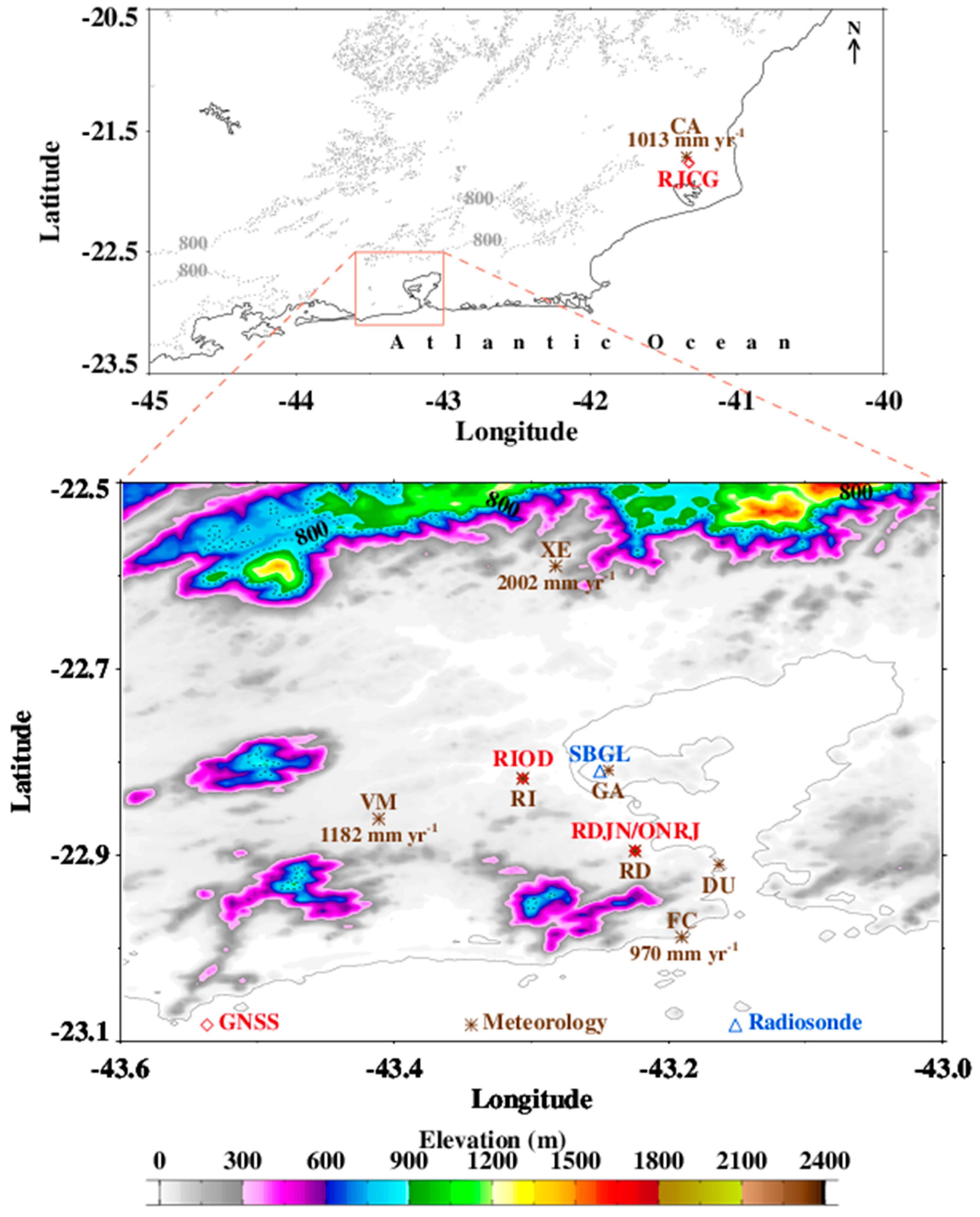
2.1. Sites and Meteorology Data

The GNSS ground-based stations used in this work, named RDJN, ONRJ, and RIOD, are located in the city of Rio de Janeiro, and RJCG is located in the city of Campos dos Goytacazes (about 230 km ENE from the city of Rio de Janeiro) (see details of each GNSS receiver and antenna in

Table 1. Altitude of the Global Navigation Satellite Systems (GNSS) sites, with the receiver and antenna types used in this work, and with their respective date of installation.

Site (Program)	Altitude (m)	Receiver Model	Antenna Model	Installation Date
RDJN (iGMAS)	39.45	- UNICORE UB4B0I	- NOV750.R4 NOVS	20 August, 2014
ONRJ	39.53	- LEICA GR25	- LEICA AR10 (773758)	4 July, 2013
(RBMC)		- TRIMBLE NETR8	- GNSS CHOKE RING (TRM59800.00)	11 March, 2015
RIOD	12.44	- LEICA GR25	- LEICA AR10 (773758)	8 August, 2013
(RBMC)		- TRIMBLE NETR9	- ZEPHYR 3 GEODETIC (TRM115000.00)	12 March, 2018
RJCG (RBMC)	14.74	- TRIMBLE NETR5	- ZEPHYR GNSS GEODETIC MODEL 2 (TRM55971.00)	11 December, 2007

). Figure 1 shows maps with the complex topography, where the elevation of 800 m is highlighted. Figure 1 includes the locations of all sites used in this study in the state of Rio de Janeiro (upper panel), a zoomed sector of the MARJ (lower panel), and the yearly rainfall averages (mm yr⁻¹) from the Instituto Nacional de Meteorologia (INMET) [35] stations. The iGMAS station RDJN was installed 4 m away from the RBMC station ONRJ in a steel pier base (3 m in height) above the concrete roof of a building in the National Observatory. The National Observatory is located on a hill about 4 km north and east of a large massive mountain and 1 km west of the Guanabara Bay. The RBMC station RIOD was installed in a concrete pillar of about 1 m in height above the roof in a building of the Instituto Brasileiro de Geografia e Estatística (IBGE), located in a valley 12 km northwest of the RDJN station and 6 km west-southwest of the Radiosonde station (internationally named as SBGL but nevertheless identified as RADS in this study) located in the Governor’s Island (Ilha do Governador) in the Guanabara Bay. The RBMC station RJCG was installed in a concrete pillar of 1.2 m height above the roof a building in the Universidade Federal Fluminense in Campos dos Goytacazes. The city of Campos dos Goytacazes is located in a flat region, although 28 km east of mountain ranges and 31 and 43 km west and north, respectively, of the Atlantic Ocean (Figure 1).

The meteorological data used, with the station locations indicated in Figure 1, are from three different sources—(i) the stations near the GNSS receivers (RD alongside the iGMAS station RDJN, and RI alongside the RBMC station named RIOD [31]); (ii) data from the INMET [35] (the stations Vila Militar (VM), Forte de Copacabana (FC), Xerém (XE), and Campos dos Goytacazes (CA); and (iii) the stations Aeroporto do Galeão (GA) and Aeroporto Santos Dumont (DU) from the Integrated Surface Database (ISD) [37,38]. The meteorological data were available in the period of February 2015–August 2018, except those from the station RI, where measurements were interrupted by late 2015.

The meteorological data from eight different stations for the year 2015 were used to test the values of the observed T and their resulting calculated surface temperature (T_s), the weighted mean temperature (T_m), and the observed and calculated surface pressure (P and P_s). The best match of meteorological values with those from RI in 2015 were chosen to calculate IWV for the station RIOD in the whole period from 2015–2018.

The data from the stations RD and RI had original time resolution of one second and one minute, respectively, while the other meteorological datasets were recorded hourly. The meteorological records were either averaged or interpolated for every 15 min to match with the time resolution of the ZTD outputs to calculate IWV.

2.2. GNSS ZTD and IWV

ZTD is defined as the propriety of the atmosphere to delay electromagnetic waves from the satellites to the receivers in the zenith direction. GNSS signals delayed in the zenith direction are divided, as shown by Bevis et al. [1], Davis et al. [39], and Saastamoinen [40], into zenith hydrostatic delay (ZHD, with the largest contribution of the dry air atmospheric gases) and zenith wet delay (ZWD, which is produced solely by the atmospheric water vapor).

$$\mathrm{ZTD}=\mathrm{ZHD}+\mathrm{ZWD},$$

(1)

where

$$\mathrm{ZHD}={10}^{-6}{\mathrm{k}}_1{\mathrm{R}}_{\mathrm{d}}\frac{{\mathrm{P}}_{\mathrm{s}}}{{\mathrm{g}}_{\mathrm{m}}},$$

(2)

${\mathrm{k}}_1$ is a refractivity constant, $R_{\mathrm{d}}$ is the gas constant of dry air, $P_{\mathrm{s}}$ is surface pressure, and ${\mathrm{g}}_{\mathrm{m}}$ is the mean gravity acceleration, which can be expressed as

$${\mathrm{g}}_{\mathrm{m}}=\frac{{\int }_0^{\infty }{\mathsf{\rho }}_{\mathrm{v}}\left(\mathrm{z}\right)\mathrm{g}\left(\mathrm{z}\right)\mathrm{dz}}{{\int }_0^{\infty }{\mathsf{\rho }}_{\mathrm{v}}\left(\mathrm{z}\right)\mathrm{dz}},$$

(3)

where ${\mathsf{\rho }}_{\mathrm{v}}$ is the water vapor density and $\mathrm{g}$ is acceleration due to gravity.

The IWV content, with the units of kg m⁻², is also referred to as precipitable water vapor (PWV), which is equivalent to the height (in mm) of liquid water obtained if the total mass of water vapor contained in an atmospheric air column of unit cross-section area that was condensed and brought to the receiver’s level.

$$\mathrm{IWV}=\underset{0}{\overset{\infty }{\int }}{\mathsf{\rho }}_{\mathrm{v}}\left(\mathrm{z}\right)\mathrm{dz}.$$

(4)

From the approximate relationship between IWV and the observed ZWD derived by Askne et al. [41],

$$\mathrm{ZWD}={10}^{-6}{\mathrm{R}}_{\mathrm{v}}\underset{0}{\overset{\infty }{\int }}{\mathsf{\rho }}_{\mathrm{v}}\left(\mathrm{z}\right)\left[{\mathrm{k}}_2^{\prime }+\frac{{\mathrm{k}}_3}{\mathrm{T}\left(\mathrm{z}\right)}\right]\mathrm{dz},$$

(5)

where ${\mathrm{k}}_2^{\prime }={\mathrm{k}}_2-{\mathrm{k}}_1\left[{\mathrm{M}}_{\mathrm{v}}/{\mathrm{M}}_{\mathrm{d}}\right]$ (K hPa⁻¹), ${\mathrm{k}}_1$ = 77.600 (K hPa⁻¹), ${\mathrm{k}}_2$ = 70.4 (K hPa⁻¹), and ${\mathrm{k}}_3$ = 3.739 × 10³ (K² hPa⁻¹) are the refractivity constants; R_v = 461.522 (J K⁻¹ kg⁻¹) is the gas constant of water vapor; M_v = 18.0152 (g mol⁻¹) is the molar mass of water vapor and M_d = 28.9644 (g mol⁻¹) is the molar mass of dry air; and T is the temperature.

Following the definition of mean temperature of the vertical air column $T_{\mathrm{m}}$ [39],

$$T_{\mathrm{m}}=\frac{{\int }_0^{\infty }{\mathsf{\rho }}_{\mathrm{v}}\left(\mathrm{z}\right)\mathrm{dz}}{{\int }_0^{\infty }\frac{{\mathsf{\rho }}_{\mathrm{v}}\left(\mathrm{z}\right)}{\mathrm{T}\left(\mathrm{z}\right)}\mathrm{dz}},$$

(6)

and combining the equation of state of water vapor, and Equations (2)–(6), as in reference [1], and following the formalism proposed by Davis et al. [39] and Saastamoinen [40], and rearranging them,

$$\mathrm{IWV}=\mathsf{\kappa }(T_{\mathrm{m}})\times \mathrm{ZWD},$$

(7)

where $\mathsf{\kappa }(T_{\mathrm{m}})$ is a function of the weighted mean temperature, expressed as

$$\mathsf{\kappa }(T_{\mathrm{m}})={10}^{-6}{\mathrm{R}}_{\mathrm{v}}\left[{\mathrm{k}}_2^{\prime }+\frac{{\mathrm{k}}_3}{T_{\mathrm{m}}}\right].$$

(8)

We also used the following equation, derived from Davis et al. [39] and Saastamoinen [40], to calculate IWV:

$${\mathrm{g}}_{\mathrm{m}}\left(\mathsf{\phi },\mathrm{H}\right)=9.784\left[\left(2\mathsf{\phi }\right)-0.00000028\mathrm{H}\right],$$

(9)

where φ and H are the latitude and the height of the surface above the ellipsoid, respectively.

To calculate T_s and P_s at the level of the receiver, to correct the differences of the height between the meteorological sensors and the GNSS receiver, we used the auxiliary equations as recommended by ICAO [42].

$${\mathrm{T}}_2={\mathrm{T}}_1+\mathsf{\alpha }\left({\mathrm{z}}_2-{\mathrm{z}}_1\right)$$

(10)

and

$${\mathrm{P}}_2={\mathrm{P}}_1{\left(\frac{{\mathrm{T}}_2}{{\mathrm{T}}_1}\right)}^{\raisebox{1ex}{$-{\mathrm{g}}_0$}\!\left/ \!\raisebox{-1ex}{${\mathsf{\alpha }R}_{\mathrm{d}}$}\right.},$$

(11)

where $\mathsf{\alpha }$ is the vertical temperature gradient (temperature lapse rate −6.5 K km⁻¹), and T₁ and P₁ are the observed temperature and pressure at the initial height $z_1$, R_d = 287.027 J K⁻¹ kg⁻¹ (including CO₂) and ${\mathrm{g}}_0$ = 9.80665 m s⁻².

The actual value for $T_{\mathrm{m}}$ is expected to change due to the dependence on surface temperature, tropospheric temperature profile, and on the vertical distribution of the atmosphere [1]. However, we adopted the common approximation of $T_{\mathrm{m}}=70.2+0.72T_{\mathrm{s}}$ [1] for the absence of frequent radiosonde and the purposes of this research.

We used GPS observation (RINEX files) data to perform a zero-differenced Precise Point Positioning (PPP) technique with Bernese GNSS Software version 5.2 [43] to estimate tropospheric parameters. The collected data were processed in 24-h sessions starting at 0000 Coordinated Universal Time (UTC) each day with data sampling of 30 s. We employed and adjusted the extended version of the PPP strategy (PPP_DEMO.PCF) to obtain high-rate tropospheric parameters with 15-min sampling. We applied the dry and wet terms of the Vienna Mapping Function 1 (VMF1, available for download at http://vmf.geo.tuwien.ac.at/) [44] together with the European Centre for Medium-Range Weather Forecasts (ECMWF)–based zenith path delays corrections. Horizontal tropospheric gradients were estimated every 24 h using the Chen-Herring gradient model [45]. We used the value of 3° for the low elevation cut-off angle in all processing data.

All ZTD estimates passed mandatory quality-control to avoid erroneous observations. Following the approach proposed by Bock et al. [46] and developed by Stepniak et al. [47], the screening procedure, aimed at detecting and removing the ZTD estimates that were physically out of range and/or less accurate value, was applied. ZTD data were screened concerning (i) the range check (reject ZTD values outside of 1 m and 3 m), (ii) the outlier check (reject ZTD values outside of median[ZTD] ± 0.5 m), (iii) σ_ZTD range check (reject σ_ZTD values outside of 0.1 mm and 6 mm), and (iv) σ_ZTD outlier check (reject σ_ZTD values > 2 × median[σ_ZTD]).

The IWV products from MODIS and radiosonde were additionally used to complement the comparisons against GNSS IWV estimates.

2.3. MODIS- and Radiosonde-Derived IWV

The MODIS MOD07 and MYD07 are products from the satellites TERRA (launched in 1999) and AQUA (launched in 2002), respectively. These products provide, among other resources, atmospheric profiles of water vapor IR-based estimates (the Total Column Precipitable Water Vapor—IR Retrieval—is identified in the MODIS products in the subset “Atmospheric Profiles”) in a 5 × 5 km resolution when at least nine Field of Views (FOVs) are cloud free (for details and downloading the dataset, see references [48,49,50,51,52]). The TERRA and AQUA satellites overpass the region of this research twice per day in the intervals of 09:00–10:45 and 22:00–23:15 and 00:30–02:30 and 12:45–14:30 local time (LT), respectively.

MODIS IWV estimates were used for areal averages and for the comparisons with GNSS IWV estimates in the nearest grid of the respective GNSS receiver.

Radiosonde-derived IWV (data obtained directly from the Wyoming University website: http://weather.uwyo.edu/upperair/sounding.html) was also used for comparisons with GNSS IWV, although the GNSS receivers were not collocated in the neighborhood of the radiosonde launching site. The Vaisala RS92-SGP [53] radiosondes are launched twice-daily before the standard times of 09:00 and 21:00 LT.

Both MODIS and radiosonde IWV estimates were used for comparisons with GNSS-derived IWV for the period from February 2015–August 2018.

3. Results

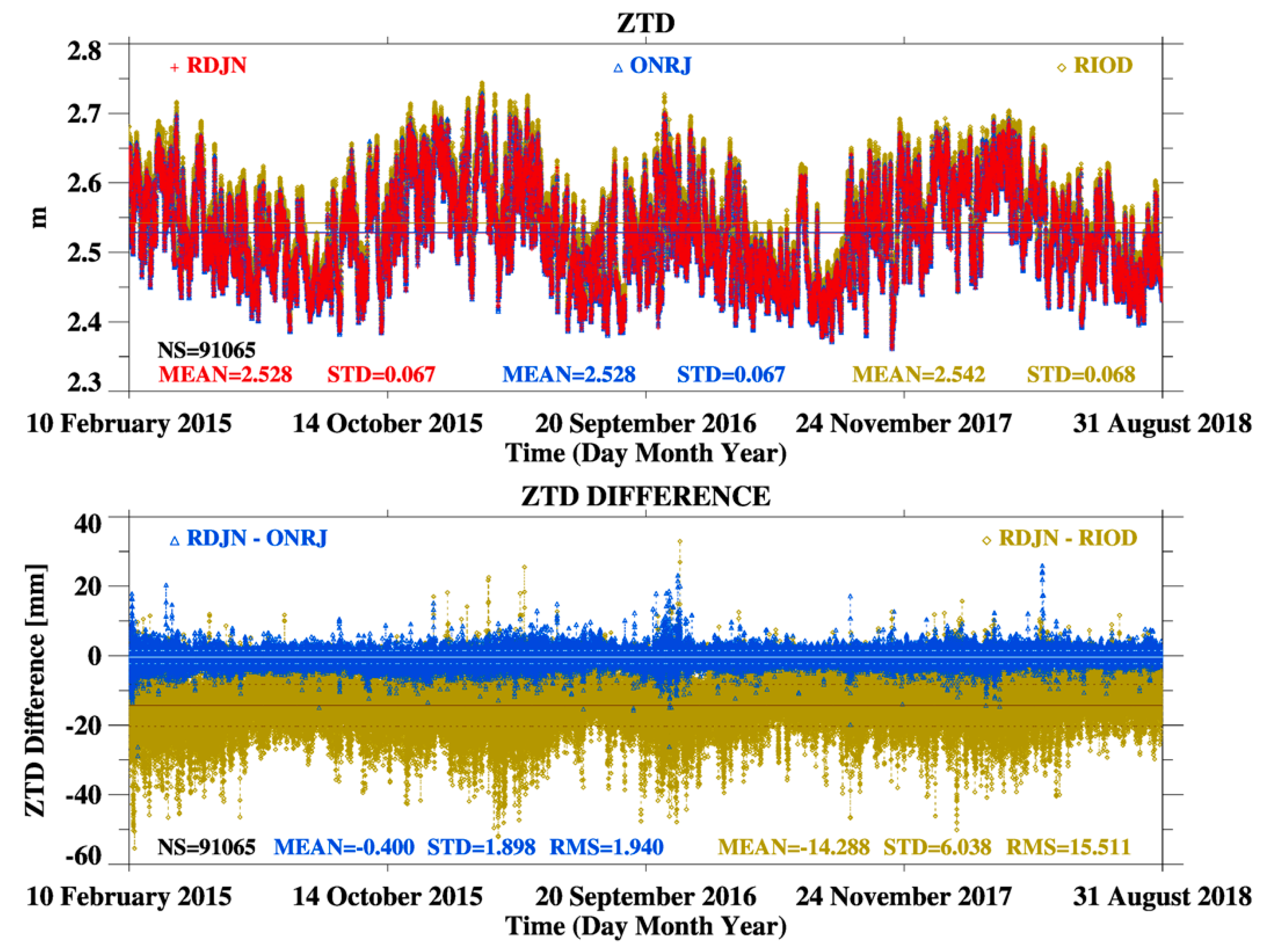
3.1. Analysis of GNSS-Derived ZTD

Variations in the elevation in a region imply differences in the distribution of GNSS-derived ZTD. We used ZTD time series from the iGMAS station and compare them with those from the RBMC stations ONRJ and RIOD. The latter stations are located 4 and 12 km away from RDJN, and they differ in −8 cm and 27 m, respectively, with respect to the elevation of RDJN (see Table 1). Figure 2 shows the time series of ZTD (top panel) and statistics ZTD differences (lower panel) from RDJN for the period of February 2015–August 2018. The long-term time series (with 91,065 samples) showed the general pattern of seasonal variations and high variability of the differences in the small scale with occasional spikes. The total ZTD averages were 2.528/2.528/2.542 m for RDJN/ONRJ/RIOD. The mean, STD, and RMS of ZTD differences between RDJN and ONRJ were −0.40 mm, 1.90 mm, and 1.94 mm, respectively; while the mean, STD, and RMS of the differences between RDJN and RIOD were −14.28 mm, 6.04 mm, and 15.51 mm, respectively. For every three-hour period, the mean difference between ZTD_RDJN and ZTD_ONRJ had the lowest (highest) values of −0.24 (−0.60) mm from 09:00–12:00 (00:00–02:45) LT; while the mean differences between ZTD_RDJN and ZTD_RIOD had the lowest (highest) values of −13.27 (−15.27) mm from 06:00–08:45 (15:00–17:45) LT. The differences between RDJN and RIOD must had first order components the differences in altitude and atmospheric conditions, as discussed in the following sections.

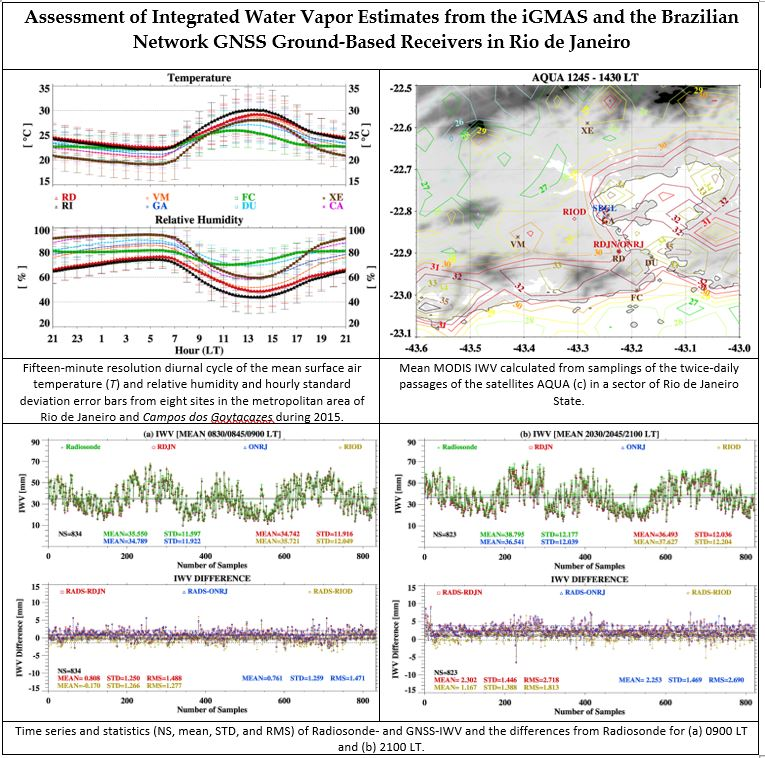
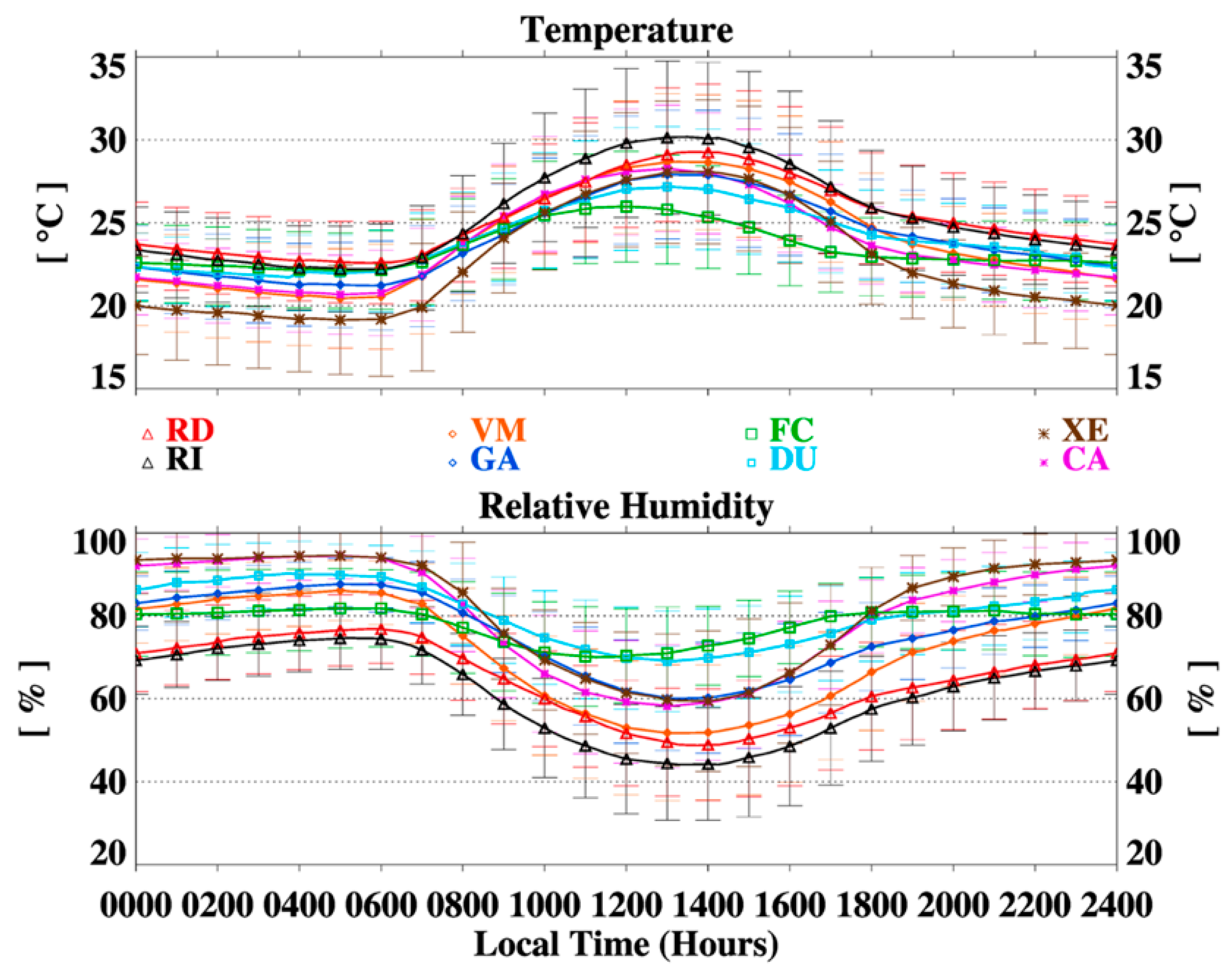
3.2. Meteorological Conditions

We analyzed the meteorological conditions prevailing in six sites in the city of Rio de Janeiro and in the stations named XE and CA located in the municipalities of Xerém and Campos dos Goytacazes (36 NNE and 233 km ENE from Rio de Janeiro), respectively. Figure 3 provides a general view of the mean (and standard deviation) of the 15-min resolution diurnal cycle of T and relative humidity (RH) during the year 2015.

It is worth noting that the meteorological variables statistics were calculated for the period of February 2015–August 2018 for all stations, except for the station RI, which became inoperant by late 2015. The mean patterns of the diurnal cycle found for the entire period (not shown) were close to those presented for the year 2015 only.

There was large variability of T and RH with a well-defined diurnal cycle in continental sites in contrast with a small amplitude of T and RH in the near-oceanic sites. Moreover, Figure 3 highlights the diurnal cycle of T and RH for the sites RI/RD against FC/XE due to their evident differences. The highest (lowest) mean values of T (RH) in the diurnal cycle were observed in the sites RI and RD (XE and FC), with expressive differences of the mean T (RH) as high as 5 °C (30%).

Large values of RH were found in the afternoon hours at FC, located by the coast, and in the nocturnal hours at XE, located near the northern mountain ranges that favor high convergence and convective activity in the foothills. (See Figure 1, which shows higher records of rainfall in XE than those in the other two sites with recorded rainfall.)

T_m is commonly used to estimate IWV [1], which is highly correlated with the observed surface T and water vapor pressure (e) [54,55]. We compared the three-hour statistics of T and e from four different inputs (available from 2015–2018) with those from the site RI that is available only in the year 2015. With these comparisons we tested T_m, and hence IWV for RIOD, and applied the best approximation of meteorological variables for that site in the entire period of this research.

Table 2. Statistics (number of samples (NS), mean, STD, root mean square (RMS), and the correlation coefficient (R)) of the differences of the variables (vars) observed T, water vapor pressure (e), T_m, and integrated water vapor (IWV) from the meteorological and GNSS data for the three-hour periods of (a) 00:00–02:45 local time (LT) and (b) 12:00–14:45 LT for the year 2015.

(a) 00:00–02:45 LT with NS = 1648
Stations:	RI	RD	VM	FC	XE
Var: T	22.700	23.072	21.086	21.936	19.483
DIFF.	Diff. (°C)	Diff. (%)	STD (K)	RMS (K)	R
RI–RD	−0.372	−1.639	0.541	0.656	0.973
RI–VM	1.613	7.108	1.425	2.152	0.856
RI–FC	0.764	3.367	1.502	1.685	0.777
RI–XE	3.217	14.173	2.415	4.022	0.657
Stations:	RI	RD	VM	FC	XE
Var: e	19.344	20.319	20.842	21.322	21.060
DIFF.	Diff. (hPa)	Diff. (%)	STD (hPa)	RMS (hPa)	R
RI–RD	−0.975	−5.043	1.008	1.403	0.954
RI–VM	−1.580	−8.166	1.929	2.493	--
RI–FC	−1.978	−10.225	1.210	2.318	0.914
RI–XE	−1.716	−8.871	2.037	2.663	0.829
Stations:	RI	RD	VM	FC	XE
Var: Tm	286.744	286.007	286.001	285.019	285.318
DIFF.	Diff. (K)	Diff. (%)	STD (K)	RMS (K)	R
RIOD (RI–RD)	0.737	0.257	0.818	1.101	0.963
RIOD (RI–VM)	0.744	0.259	0.606	0.959	0.978
RIOD (RI–FC)	1.726	0.602	1.655	2.391	0.810
RIOD (RI–XE)	1.426	0.497	0.777	1.624	0.961
Stations:	RIOD(RI)	RIOD(RD)	RIOD(VM)	RIOD(FC)	RIOD(XE)
Var: IWV	37.624	37.592	37.301	37.299	37.245
DIFF.	Diff. (K)	Diff. (%)	STD (K)	RMS (K)	R
RIOD (RI–RD)	0.032	0.085	0.067	0.074	1.000
RIOD (RI–VM)	0.323	0.858	0.108	0.340	1.000
RIOD (RI–FC)	0.325	0.865	0.204	0.384	1.000
RIOD (RI–XE)	0.379	1.009	0.204	0.431	1.000
(b) 12:00–14:45 LT with NS = 3133
Stations:	RI	RD	VM	FC	XE
Var: T	29.543	28.590	28.159	25.103	27.519
DIFF.	Diff. (°C)	Diff. (%)	STD (K)	RMS (K)	R
RI–RD	0.953	3.225	1.218	1.546	0.965
RI–VM	1.384	4.685	1.007	1.712	0.976
RI–FC	4.440	15.027	2.872	5.288	0.763
RI–XE	2.024	6.849	1.253	2.380	0.958
Stations:	RI	RD	VM	FC	XE
Var: e	18.133	19.233	19.773	22.997	21.871
DIFF.	Diff. (hPa)	Diff. (%)	STD (hPa)	RMS (hPa)	R
RI–RD	−1.100	−6.067	1.265	1.676	0.926
RI–VM	−1.658	−9.144	3.431	3.810	--
RI–FC	−4.863	−26.820	2.336	5.395	0.728
RI–XE	−3.738	−20.612	1.800	4.148	0.884
Stations:	RI	RD	VM	FC	XE
Var: Tm	288.139	287.565	287.224	285.081	286.736
DIFF.	Diff. (K)	Diff. (%)	STD (K)	RMS (K)	R
RIOD (RI–RD)	0.574	0.199	0.877	1.048	0.965
RIOD (RI–VM)	0.914	0.317	0.725	1.167	0.976
RIOD (RI–FC)	3.058	1.061	2.068	3.692	0.763
RIOD (RI–XE)	1.403	0.487	0.902	1.668	0.958
Stations:	RIOD(RI)	RIOD(RD)	RIOD(VM)	RIOD(FC)	RIOD(XE)
Var: IWV	37.194	37.040	36.903	36.364	36.973
DIFF.	Diff. (mm)	Diff. (%)	STD (mm)	RMS (mm)	R
RIOD (RI–RD)	0.154	0.414	0.143	0.210	1.000
RIOD (RI–VM)	0.291	0.783	0.141	0.324	1.000
RIOD (RI–FC)	0.830	2.231	0.368	0.908	1.000
RIOD (RI–XE)	0.221	0.595	0.184	0.288	1.000

shows the statistics for two periods (00:00–02:45 LT and 12:00–14:45 LT) of the variables (vars) T, e, and T_m for RI and IWV in relation with other four sites.

The comparisons of the matches were not linear, but they had significant different values of the variables within the sites, except the comparisons against those of the site RD. The meteorological conditions for the matches RI and RD were reasonably similar, with lower differences and higher statistical significance than those of RI and the other sites.

The mean ΔT (Δe), STD, and RMS were about −0.4 °C, 0.5 °C, and 0.7 °C (−1.98 hPa, 1.01 hPa, and 1.40 hPa), respectively for 00:00–02:45 LT; and the mean ΔT (Δe), STD, and RMS were about 1.0 °C, 1.2 °C, and 1.7 °C (−1.10 hPa, 1.26 hPa, and 1.77 hPa), respectively for 12:00–14:45 LT. The differences between the matches, in those two intervals, led to about 0.7/0.6 K and 0.03/0.15 mm, respectively, for ΔT_m and ΔIWV. The comparisons between the matches RI/XE and RI/FC showed high ΔT (Δe), up to 3.2/4.4 °C (−1.72/−4.89 hPa), led to relatively high values of 1.4/3.1 K and 0.38/0.83 mm for ΔT_m and ΔIWV, respectively.

From these comparisons, the best meteorological data used to estimate T_m, and hence IWV for the station RIOD in the period 2015–2018 were from the meteorological station RD. These comparisons showed low ΔT and Δe, less spread, and high accuracy between the matches RD and RI, and hence low ΔT_m and ΔIWV, in the year 2015.

3.3. MODIS- Versus GNSS-Derived IWV

Water vapor measurements from both MODIS satellites (TERRA and AQUA) provide an insightful complementary tool to analyze IWV jointly with GNSS-derived IWV. Figure 4 shows the temporal mean IWV of the daytime and nighttime overpasses of either MODIS TERRA or AQUA satellite in the absence of clouds in the MARJ. Two main patterns are observed in these panels—(i) a general underestimation of IWV in the nighttime averages and (ii) a shifting of the highest values over the continent and over the ocean from daytime to nighttime. IWV distributions were marked by the largest mean values along the Atlantic coastline toward the upslopes of the mountain ranges during the daytime intervals of 09:30–10:45 (Figure 4b) and 12:45–12:30 LT (Figure 4c). The nocturnal averages in the intervals of 00:30–02:30 (Figure 4a) and 22:00–23:15 LT (Figure 4d) showed the largest IWV values in the atmosphere above the oceanic surface, indicating the presence of shifting breeze circulations in the diurnal cycle.

Table 3. Statistics (NS, mean, STD, RMS, and R) of estimates in the nearest point of MODIS IWV and GNSS IWV differences in the stations RDJN, RIOD, and RJCG. Grey shaded background highlights the nocturnal from the diurnal passages of the satellites AQUA and TERRA.

Local Time	AQUA		RDJN	Local Time	TERRA	RDJN
00:30–02:30	25.085		28.016	09:30–10:45	28.942	27.816
12:45–14:30	30.179		29.408	22:00–23:15	23.617	28.316
MODIS	NS	Diff. (mm)	Diff. (%)	STD (mm)	RMS (mm)	R
AQUA (night)	223	–2.931	–10.462	4.999	5.785	0.841
TERRA (day)	217	1.125	4.046	5.273	5.379	0.887
AQUA (day)	242	0.771	2.622	5.578	5.620	0.891
TERRA (night)	145	–4.699	–16.596	4.406	6.431	0.889
Local Time	AQUA		RIOD	Local Time	TERRA	RIOD
00:30–02:30	26.242		31.143	09:30–10:45	29.564	30.239
12:45–14:30	30.707		31.461	22:00–23:15	23.456	30.768
MODIS	NS	Diff. (mm)	Diff. (%)	STD (mm)	RMS (mm)	R
AQUA (night)	234	–4.901	–15.736	4.683	6.772	0.883
TERRA (day)	278	–0.675	–2.232	4.729	4.769	0.920
AQUA (day)	324	–0.755	–2.399	6.499	6.533	0.873
TERRA (night)	204	–7.313	–23.767	4.371	8.514	0.887
Local Time	AQUA		RJCG	Local Time	TERRA	RJCG
00:30–02:30	25.687		31.627	09:30–10:45	29.575	31.491
12:45–14:30	31.495		32.582	22:00–23:15	23.130	31.778
MODIS	NS	Diff. (mm)	Diff. (%)	STD (mm)	RMS (mm)	R
AQUA (night)	266	–5.940	–23.123	3.904	7.104	0.880
TERRA (day)	258	–1.916	–6.477	4.287	4.688	0.928
AQUA (day)	290	–1.087	–3.452	5.107	5.212	0.911
TERRA (night)	244	–8.649	–37.391	3.917	9.491	0.890

presents the statistics of the IWV differences between MODIS and GNSS estimates. The nearest grid with MODIS IWV from the two daily passages of each satellite TERRA or AQUA were simultaneously collocated with the data from the GNSS stations RDJN/RIOD/RJCG. There was a general trend of MODIS-IWV to follow GNSS-IWV with relatively high correlation coefficient (above 0.84) for all matches. The differences between IWV_MODIS and IWV_RDJN in the daytime comparisons were from 0.8–1.1 mm (equivalent to percentage differences of about 2.6–4%); while the differences of IWV_MODIS against IWV_RIOD and IWV_RJCG were from −2 to −0.7 (equivalent to percentage differences of about −6.5% to −2.2%). (The comparisons of MODIS against GNSS IWV in intervals of low, intermediate, and high IWV values (not shown) presented high spam of the differences, more spread, and low correlation between the matches, probably related with small number of samples considered.) Although the STD and RMS were relatively high (from 4.3–6.5 mm) for the diurnal estimates, the mean differences and correlation results were comparable with the acceptable ranges observed in previous comparisons of MODIS and GNSS IWV, such as those observed by Liu et al. [9], Vaquero-Martínez et al. [10], Alraddawi et al. [56], and Cimini et al. [57]. However, MODIS predominantly underestimated IWV against all GNSS estimates in the nocturnal passages, as observed in the areal averages. High percentages of the differences (of −37.4% to −10.5% from MODIS) correspondent to mean differences from −8.6 mm to −3 mm, STD from 4–5 mm (slightly lower than for daytime comparisons) and RMS from about 4.7–9.5 mm.

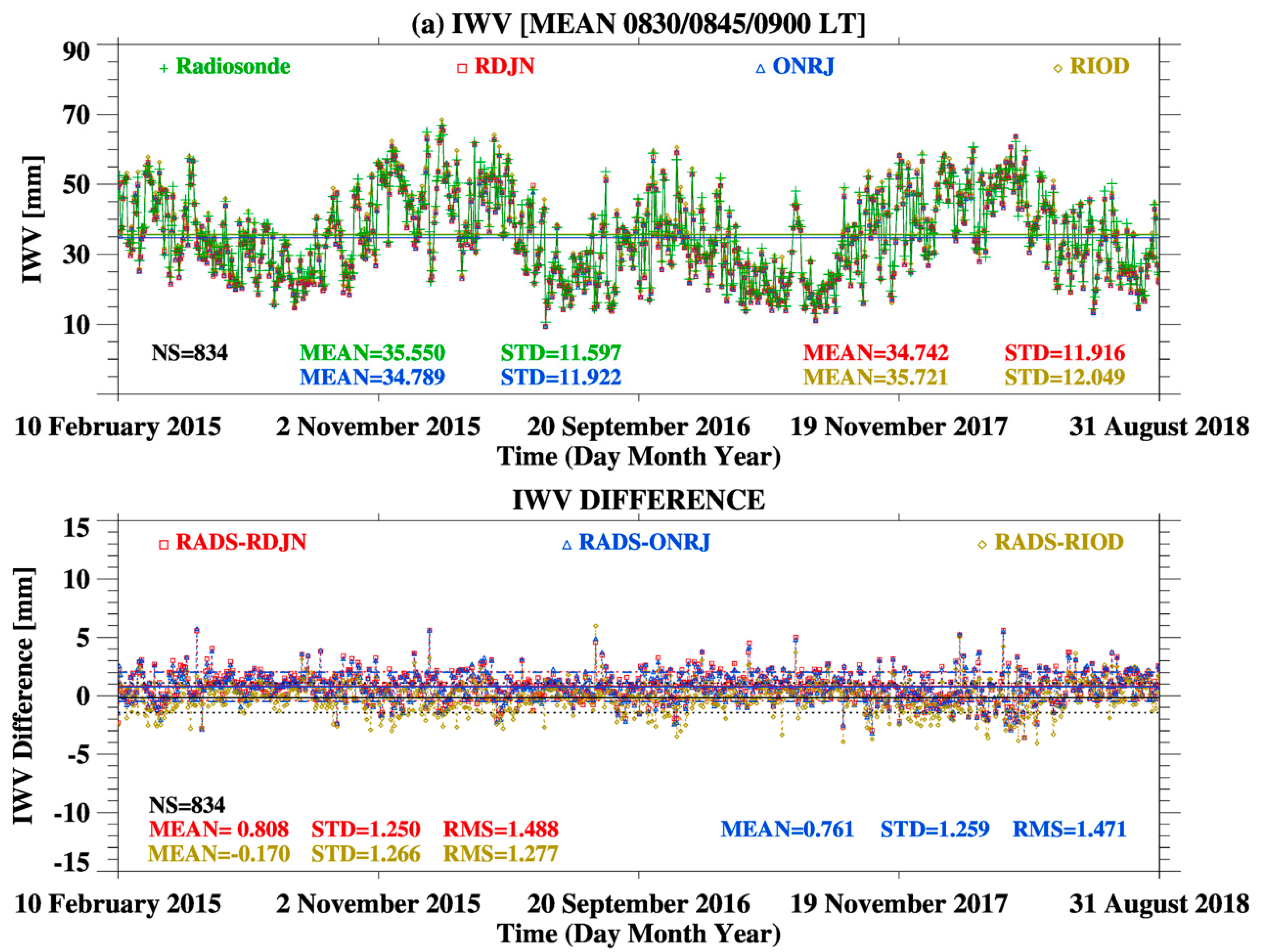
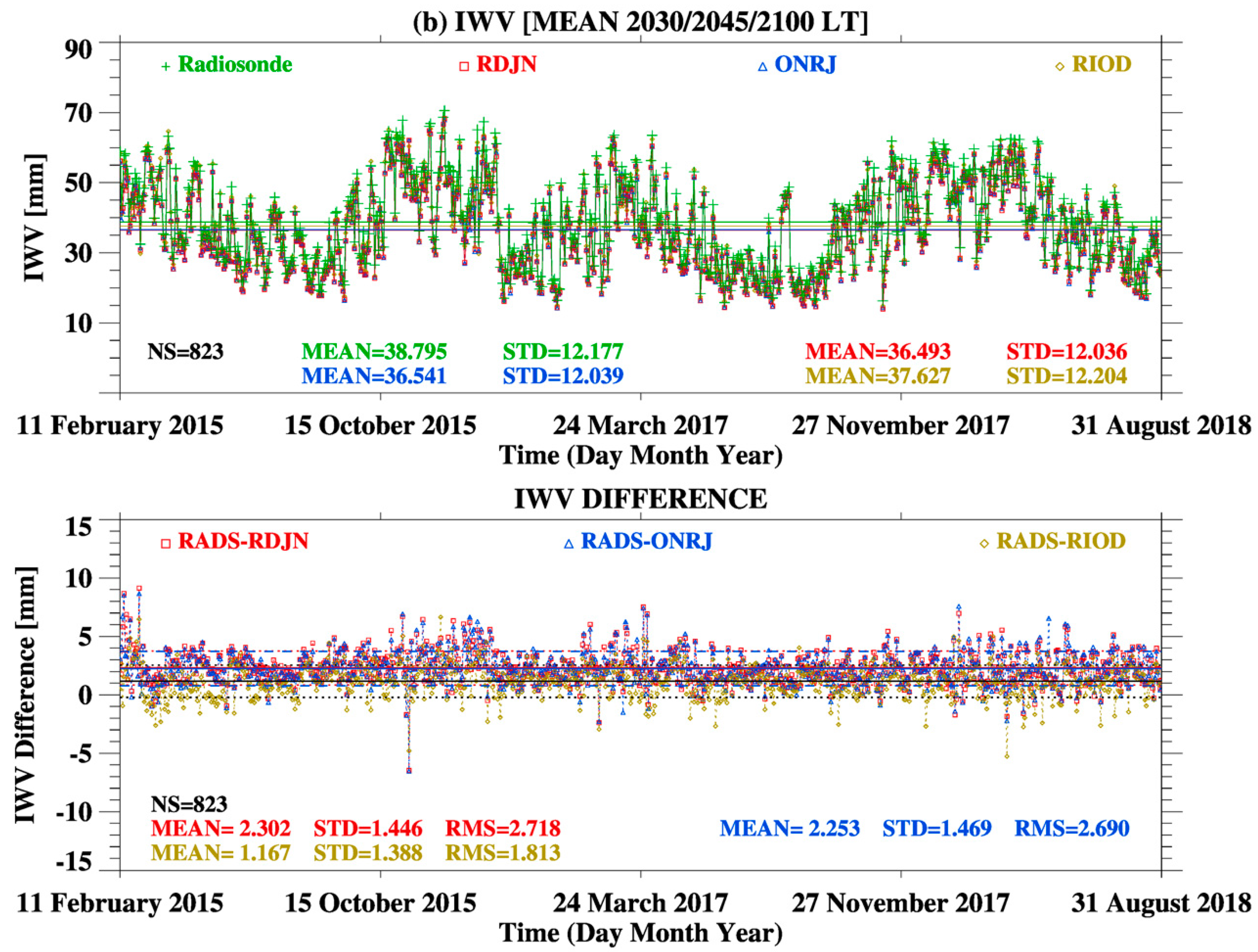
3.4. Radiosonde- Versus GNSS-Derived IWV

The comparisons of GNSS-IWV with the twice-daily radiosonde-IWV (RADS 09:00 LT and 21:00 LT) are used to evaluate the performances of IWV estimates for RDJN, ONRJ, and RIOD. Despite the disadvantage of the non-instantaneous measurements of the radiosonde observations, since the soundings are launched about 30 min before the standard time (ST), and the soundings last from 1–2 h [58], we first tested the mean differences between GNSS-IWV at the ST of the radiosonde launching (i) and four different scenarios—(ii) 30 min before ST, (iii) 15 min before ST, (iv) 15 min after ST, and (v) 30 min after ST (

Table 4. NS, mean, STD, and RMS of the differences between GNSS IWV on the ST (scenario (i)) and the scenarios (ii) 30 min before ST, (iii) 15 min before ST, (iv) 15 min after ST, (v) 30 min after ST, and the mean (shaded rows) of the scenarios (i), (ii), and (iii) for the two daily soundings of (a) 09:00 LT and (b) 21:00 LT in the period from February 2015–August 2018.

(a) 0900 LT	RDJN(i) = 34.745		ONRJ(i) = 34.778		RIOD(i) = 35.720
NS = 834	Diff. (mm)	Diff. (%)	STD (mm)	RMS (mm)	R
RDJN(i)–RDJN(ii)	−0.004	−0.012	0.654	0.653	0.999
ONRJ(i)–ONRJ(ii)	−0.025	−0.073	0.641	0.641	0.999
RIOD(i)–RIOD(ii)	0.003	0.010	0.798	0.798	0.998
RDJN(i)–RDJN(iii)	0.010	0.030	0.394	0.394	0.999
ONRJ(i)–ONRJ(iii)	−0.008	−0.023	0.398	0.398	0.999
RIOD(i)–RIOD(iii)	−0.008	−0.021	0.502	0.502	0.999
RDJN(i)–RDJN(iv)	−0.005	−0.014	0.366	0.366	--
ONRJ(i)–ONRJ(iv)	−0.004	−0.010	0.386	0.385	--
RIOD(i)–RIOD(iv)	0.004	0.012	0.468	0.468	--
RDJN(i)–RDJN(v)	−0.031	−0.088	0.629	0.629	--
ONRJ(i)–ONRJ(v)	−0.027	−0.078	0.662	0.662	--
RIOD(i)–RIOD(v)	−0.028	−0.078	0.784	0.784	--
RDJN(i)–RDJN(vi)	0.002	0.006	0.337	0.337	1.000
ONRJ(i)–ONRJ(vi)	−0.011	−0.032	0.332	0.332	1.000
RIOD(i)–RIOD(vi)	−0.001	−0.004	0.414	0.414	0.999
(b) 2100 LT	RDJN(i) = 36.480		ONRJ(i) = 36.530		RIOD(i) = 37.579
NS = 823	Diff. (mm)	Diff. (%)	STD (mm)	RMS (mm)	R
RDJN(i)–RDJN(ii)	−0.030	−0.082	0.702	0.702	0.998
ONRJ(i)–ONRJ(ii)	−0.023	−0.062	0.706	0.706	0.998
RIOD(i)–RIOD(ii)	−0.109	−0.291	0.808	0.815	0.998
RDJN(i)–RDJN(iii)	−0.011	−0.029	0.337	0.337	1.000
ONRJ(i)–ONRJ(iii)	−0.013	−0.036	0.338	0.338	1.000
RIOD(i)–RIOD(iii)	−0.036	−0.096	0.400	0.401	0.999
RDJN(i)–RDJN(iv)	0.025	0.068	1.140	1.140	--
ONRJ(i)–ONRJ(iv)	0.007	0.018	1.146	1.146	--
RIOD(i)–RIOD(iv)	−0.251	−0.668	1.607	1.626	--
RDJN(i)–RDJN(v)	0.032	0.088	1.218	1.218	--
ONRJ(i)–ONRJ(v)	0.005	0.014	1.202	1.201	--
RIOD(i)–RIOD(v)	−0.231	−0.614	1.607	1.622	--
RDJN(i)–RDJN(vi)	−0.013	−0.037	0.332	0.332	1.000
ONRJ(i)–ONRJ(vi)	−0.012	−0.033	0.334	0.334	1.000
RIOD(i)–RIOD(vi)	−0.049	−0.129	0.385	0.388	1.000

). The mean differences between IWV at ST and those scenarios were quite small, with low percentage of the differences, and high correlation coefficient—nearly unbiased especially in the stations RDJN/ONRJ. The amplitudes of the differences between the scenarios for morning soundings were equal or lesser than 0.031 mm, and STD/RMS decayed from 0.641/0.784 (ii) to 0.394/0.502 (iii) and increased symmetrically from (iv) and (v) matches. The differences for the nocturnal soundings had amplitudes equal or lesser than 0.251 mm, with similar decaying compared with that in 09:00 LT, but they increased up to 1.140/1.607 mm in the matches (iv) and (v).

According to a general view of these results, there were lower biases, lesser spread, and higher accuracy in the comparisons between IWV(ST) and IWV(ST-15 min) than between IWV(ST) and others matches after ST. Therefore, the IWV differences between the scenario (i) and the scenarios (ii) and (iii) were lesser spread and had higher accuracy than against those of (iv) and (v). We used an additional scenario (vi) as the mean IWV estimates of the scenarios (i), (ii), and (iii) (see the highlighted lines in Table 4) to compare with those from radiosonde at the ST.

Though the IWV differences between RADS minus GNSS_[ST] and RADS minus GNSS_{[mean(ST-30/ST-15/ST)]} were from −0.049–0.002 mm, but STD and RMS were from 0.3–0.4 mm. Furthermore, considering that approximately 90% of water vapor distribution is located in the lower troposphere [58,59], we had chosen the mean as an ideal values of GNSS-IWV. The mean from the time of launching to the time radiosondes reach the level of 500 hPa (correspondent to the first 5 km above mean sea level), approximately on the ST, could be used as a reasonable estimate to be used for comparison with non-instantaneous radiosonde IWV. For the above, we adopted scenario (vi) for the GNSS IWV to compare them with radiosonde IWV.

Figure 5 shows the time series and statistics of IWV differences between RADS (09:00 and 21:00 LT) and RDJN/ONRJ/RIOD (mean of the estimates at 08:30, 08:45, and 09:00 LT and the mean of the estimates at 20:30, 20:45, and 21:00 LT). There was a contrasting behavior between the two daily soundings, where radiosonde IWV estimates were higher than those of all three GNSS estimates, except against RIOD at 09:00 LT.

The mean differences between IWV_RADS and IWV_RDJN/IWV_ONRJ/ IWV_RIOD at 0900 LT were 0.81/0.76/–0.17 mm, with STD 1.25/1.26/1.27 mm, and RMS 1.49/1.47/1.28 mm. At nighttime, the mean IWV_RADS minus IWV_RDJN/IWV_ONRJ/IWV_RIOD were 2.30/2.25/ 1.17 mm, with STD of 1.45/1.47/1.39 mm, and RMS of 2.72/2.69/1.81 mm.

The statistics applied for three intervals of soundings of low moisture (IWV_RADS ≤ 30 mm), intermediate moisture (30 mm < IWV_RADS < 50 mm), and high moisture (IWV_RADS ≥ 50 mm) are shown in

Table 5. Statistics (NS, mean, STD, RMS, and R) of radiosonde estimates for IWV intervals of (a) low moisture (IWV_RADS ≤ 30 mm), (b) intermediate moisture (30 mm < IWV_RADS < 50 mm), and (c) high moisture (IWV_RADS ≥ 50 mm) for the two-daily soundings in the period from February 2015–August 2018.

(a) Low Moisture: RADS IWV ≤ 30 mm
ST	RADS		RDJN	ONRJ	RIOD
0900 LT	23.345		22.274	22.298	23.072
NS = 300	Diff. (mm)	Diff. (%)	STD (mm)	RMS (mm)	R
RADS–RDJN	1.071	4.586	0.961	1.438	0.976
RADS–ONRJ	1.047	4.483	0.946	1.410	0.976
RADS–RIOD	0.273	1.169	1.001	1.036	0.975
ST	RADS		RDJN	ONRJ	RIOD
2100 LT	24.657		22.618	22.665	23.452
NS = 238	Diff. (mm)	Diff. (%)	STD (mm)	RMS (mm)	R
RADS–RDJN	2.040	8.273	0.994	2.268	0.959
RADS–ONRJ	1.993	8.082	1.013	2.235	0.957
RADS–RIOD	1.205	4.889	1.067	1.609	0.954
(b) Intermediate Moisture: 30 mm < RADS IWV < 50 mm
ST	RADS		RDJN	ONRJ	RIOD
0900 LT	38.980		38.229	38.292	39.306
NS = 415	Diff. (mm)	Diff. (%)	STD (mm)	RMS (mm)	R
RADS–RDJN	0.751	1.925	1.328	1.524	0.976
RADS–ONRJ	0.688	1.764	1.334	1.499	0.975
RADS–RIOD	−0.326	−0.838	1.286	1.325	0.977
ST	RADS		RDJN	ONRJ	RIOD
2100 LT	39.464		37.147	37.184	38.356
NS = 409	Diff. (mm)	Diff. (%)	STD (mm)	RMS (mm)	R
RADS–RDJN	2.317	5.872	1.429	2.721	0.970
RADS–ONRJ	2.280	5.777	1.475	2.714	0.968
RADS–RIOD	1.108	2.809	1.392	1.778	0.972
(c) High Moisture: RADS IWV ≥ 50 mm
ST	RADS		RDJN	ONRJ	RIOD
0900 LT	54.364		54.017	54.063	55.111
NS = 119	Diff. (mm)	Diff. (%)	STD (mm)	RMS (mm)	R
RADS–RDJN	0.347	0.638	1.454	1.489	0.927
RADS–ONRJ	0.301	0.553	1.499	1.522	0.924
RADS–RIOD	−0.747	−1.375	1.435	1.612	0.934
ST	RADS		RDJN	ONRJ	RIOD
2100 LT	56.361		53.739	53.814	55.107
NS = 176	Diff. (mm)	Diff. (%)	STD (mm)	RMS (mm)	R
RADS–RDJN	2.621	4.651	1.879	3.222	0.913
RADS–ONRJ	2.547	4.518	1.873	3.158	0.913
RADS–RIOD	1.254	2.225	1.726	2.129	0.925

, respectively in the panels (a), (b), and (c).

The comparisons between RADS and RDJN/ONRJ/RIOD were similar to those for all IWV estimates described above. Radiosonde IWV was consistently 2.0/2.3/2.6 mm higher than those of GNSS_RDJN (and GNSS_ONRJ), and 1.2/1.1/1.2 mm higher than those of GNSS_RIOD in the intervals (a)/(b)/(c) at nighttime. As for the daytime soundings, IWV_RADS was about 1.0/1.6/2.2 (calculated by Diff.₂₁₀₀ minus Diff.₀₉₀₀) mm (or 4.0/4.0/3.9%) lower than it was expected in the interval (a)/(b)/(c) if not considering dry bias.

3.5. Space and Temporal Distributions of GNSS IWV in Rio de Janeiro

The estimates of GNSS-derived IWV for the data available in the city of Rio de Janeiro from February 2015–August 2018 are presented in this section.

Table 6. Statistics (NS, Mean, STD, RMS, and R) of the IWV differences between RDJN and ONRJ and RIOD for every three hours and the whole period from February 2015–August 2018.

00:00−02:45 LT	RDJN = 36.137		ONRJ = 36.238	RIOD = 37.267
NS = 11521	Diff. (mm)	Diff. (%)	STD (mm)	RMS (mm)	R
RDJN–ONRJ	−0.101	−0.278	0.310	0.326	1.000
RDJN–RIOD	−1.130	−3.126	0.915	1.454	0.997
03:00−05:45 LT	RDJN = 35.441		ONRJ = 35.531	RIOD = 36.520
NS = 11428	Diff. (mm)	Diff. (%)	STD (mm)	RMS (mm)	R
RDJN–ONRJ	−0.090	−0.253	0.267	0.282	1.000
RDJN–RIOD	−1.079	−3.043	0.838	1.366	0.998
06:00−08:45 LT	RDJN = 34.995		ONRJ = 35.074	RIOD = 35.997
NS = 11493	Diff. (mm)	Diff. (%)	STD (mm)	RMS (mm)	R
RDJN–ONRJ	−0.079	−0.226	0.278	0.289	1.000
RDJN–RIOD	−1.003	−2.865	0.845	1.311	0.998
09:00−11:45 LT	RDJN = 34.906		ONRJ = 34.950	RIOD = 35.955
NS = 10900	Diff. (mm)	Diff. (%)	STD (mm)	RMS (mm)	R
RDJN–ONRJ	−0.044	−0.125	0.291	0.294	1.000
RDJN–RIOD	−1.049	−3.004	0.957	1.420	0.997
12:00−14:45 LT	RDJN = 35.295		ONRJ = 35.353	RIOD = 36.559
NS = 10825	Diff. (mm)	Diff. (%)	STD (mm)	RMS (mm)	R
RDJN–ONRJ	−0.057	−0.162	0.322	0.327	1.000
RDJN–RIOD	−1.264	−3.580	1.127	1.693	0.996
15:00−17:45 LT	RDJN = 36.172		ONRJ = 36.219	RIOD = 37.533
NS = 11164	Diff. (mm)	Diff. (%)	STD (mm)	RMS (mm)	R
RDJN–ONRJ	−0.046	−0.128	0.309	0.312	1.000
RDJN–RIOD	−1.360	−3.760	1.096	1.747	0.996
18:00−20:45 LT	RDJN = 36.778		ONRJ = 36.825	RIOD = 38.050
NS = 11251	Diff. (mm)	Diff. (%)	STD (mm)	RMS (mm)	R
RDJN–ONRJ	−0.048	−0.129	0.326	0.329	1.000
RDJN–RIOD	−1.273	−3.461	1.052	1.651	0.996
21:00−23:45 LT	RDJN = 36.732		ONRJ = 36.820	RIOD = 38.017
NS = 11555	Diff. (mm)	Diff. (%)	STD (mm)	RMS (mm)	R
RDJN–ONRJ	−0.088	−0.238	0.355	0.366	1.000
RDJN–RIOD	−1.285	−3.497	1.006	1.632	0.997
TOTAL MEAN	RDJN		ONRJ	RIOD
(mm)	35.676		35.742	36.848
NS = 85451	Diff. (mm)	Diff. (%)	STD (mm)	RMS (mm)	R
RDJN–ONRJ	−0.067	−0.187	0.302	0.309	1.000
RDJN–RIOD	−1.172	−3.285	0.982	1.529	0.997

shows IWV statistics for each three-hour period and for the entire dataset. High correlations between IWV_RDJN versus IWV_ONRJ and IWV_RDJN versus IWV_RIOD were observed, so that the periods of the day of maxima IWV in all three locations occurred from the afternoon to nocturnal hours, and minima occurred from dawn to noon hours, with amplitude of the diurnal cycle of 1.872, 1.875, and 2.095 mm for RDJN, ONRJ, and RIOD, respectively. Slightly low correlation coefficient (0.996) between RDJN and RIOD was observed in the period of the day of increasing rate of IWV from 12:00–21:00 LT, in comparison with the period from nocturnal–morning hours.

The minimum (maximum) mean difference between IWV_RDJN and IWV_ONRJ were –0.101 (–0.044) mm for the time interval of 00:00–02:45 (09:00–11:45) LT, while the total mean, STD, and RMS were –0.067 mm, 0.302 mm, and 0.309 mm, respectively. More significant differences were found between IWV_RDJN and IWV_RIOD (comparing with those of the latter match), with the largest amplitude of the mean differences in the afternoon to evening hours (IWV_RDJN was 1.360 mm lower than IWV_RIOD in the period 15:00–17:45 LT), and the lowest amplitude of the mean differences in the nocturnal to morning hours (IWV_RDJN was 1.003 mm lower than IWV_RIOD from 06:00–08:45 LT) for the three-hour periods. The statistics of the differences between IWV_RDJN and IWV_RIOD for the entire dataset presented mean, STD, and RMS of −1.172 mm, 0.982 mm, and 1.529 mm, respectively.

4. Discussion

The variabilities of the meteorological conditions at surface and water vapor content in the atmosphere showed important aspects in the MARJ. Despite the fact that the RDJN and ONRJ receivers being located on the roof of the same building (though under the same meteorological conditions), they served as control measurements of the main dataset of this work. The long time series of ZTD and the statistics of ZTD_RDJN and ZTD_ONRJ showed relatively small mean difference, STD, and RMS, respectively −0.4 mm, 1.9 mm, and 1.9 mm. A robust control experiment could provide accurate explanations of the differences between ZTD_RDJN and ZTD_ONRJ, whether they were primary related to instrumental errors or they were due to different receiver brand and model, hardware, phase center variations, strategies used, and/or multipath effect, such as those indicated in Jarlemark et al. [60], King et al. [61], and Ning et al. [62,63] (see also references [16,64]).

RDJN and RIOD sites were not necessarily under the same atmospheric conditions as RDJN and ONRJ sites were. Concerning ZTD statistics for the matches RDJN and RIOD, there were higher values for the mean difference, STD, and RMS (−14.3 mm, 6.0 mm, and 15.5 mm, respectively) as expected, due primarily to differences in elevation of the sites (RDJN is located on a small hill and RIOD in a valley), distances to the mountain ranges or the Atlantic Ocean, and the meteorological conditions between these two sites located 12 km apart from each other.

High variability of mean 15-min diurnal cycle of T and RH were found between the sites. T (RH) mean differences as high as 5 °C (30%) between, e.g., the sites RD/RI and FC/XE could be related with the occurrences of heat islands that have important effects in human weather comfortability and the formation of extreme weather events contributing to significant variability in the T_m, commonly used to estimate IWV. The spatiotemporal variabilities of T between the sites analyzed in this work corroborate with the observations of Lucena et al. [26,27,28] that mapped urban, suburban, and rural heat islands in the MARJ. These studies indicated that the temperatures of the surface and the air near the surface in the heat islands were much higher than those in the surrounding (vegetated or near the coast) areas and were related with extreme rainfall events. Thus, the relation between the occurrence of heat islands and the meteorological variables such as T, winds, and precipitation, could lead to a heterogeneous distribution of water vapor as well. Mean differences in T and e, up to 4.4 °C and −4.89 hPa, respectively, between the matches RI and FC, led to mean differences as high as 3.1 K for T_m and hence 0.83 mm for IWV.

The performance of MODIS MOD07 and MYD07 products, from respectively the satellites TERRA and AQUA, provided a reasonably good representation of the spatial mean distribution of IWV for the daylight passages in absence of clouds. IWV comparisons between the products from TERRA and AQUA and those from GNSS had mean differences of −2.4 mm to −0.7 mm (about −6% to 2% for MODIS against RJCG and RIOD) and 0.8–1.1 mm (about 2.6–4.0% for MODIS against RDJN) during daytime hours. However, some discrepancies were observed in the nocturnal samplings used in the comparisons, with a mean offset of −9 mm to −3 mm (about −37% to −10%) of MODIS with respect to GNSS.

The space distribution of IWV can be inferred from the long-term averages of each interval of the passages of the satellites TERRA and AQUA. Spatial differences were more evident in the daytime intervals of 09:30–10:45 and 12:45–14:30 LT, where the highest mean values of IWV were located along the oceanic coast toward the upslopes of the mountain ranges. This approximate south–north configuration of the mean IWV variation can be explained by the occurrence of daytime convection influenced by land heating, such as the heat islands identified by Lucena et al. [26,27,28], and the convergence of the southerly and easterly sea breezes that cause maxima rainfall from the coastline to the upslopes of the mountain ranges during the late afternoon to nocturnal hours, as observed by Dereczynski et al. [24] and Mota and Song [25].

As consequence of the inhomogeneity of altitude and meteorological conditions of the collocated stations used in this work, we observed that the atmosphere above RADS (located in an island) were about 2.3 mm wetter than above RDJN (located on a urban small hill) and 1.2 mm wetter than above RIOD (located in a urban valley) at 21:00 LT. The IWV differences between RDJN and RIOD remained consistently around 1.1 mm in the daytime, while IWV_RADS estimates would be 1.4 mm (or 3.7%) lower than it was expected in the absence of bias, as observed comparable underestimation order of magnitude by Sapucci et al. [65] and Turner et al. [66] (see references [15,67,68,69,70,71,72]). However, we cannot discard bias in GNSS IWV due to some other influences that were not computed in this work, and the different meteorological conditions in the sites. The above lead us to recommend that comparisons of radiosonde IWV should consider separated daylight and nighttime analyses and the GNSS receiver should be collocated near the radiosonde launching site so the comparisons would be based in measurements of the same atmosphere.

Despite the distances between the stations RADS–RDJN/ONRJ and RADS–RIOD of 10 and 6 km, respectively, which contribute to meteorological differences in water vapor spatial distribution measured by GNSS receivers, the STD of the differences were below 3 mm, as discussed by Bianchi et al. [17].

The spatiotemporal distribution of IWV was analyzed by the time series and the three-hour averages. The maxima GNSS IWV occur in the period from the afternoon to nocturnal hours, while the minima occur from dawn to noon hours, consonant with the periods of maxima and minima rainfall observed by Mota and Song [25] in the region. The consistent mean IWV difference between the sites RDJN and RIOD of −1.2 mm is similar to the results obtained by Bianchi et al. [17], who found −1.2 mm difference between IWV_ONRJ and IWV_RIOD in the period of about seven years from 2007.

The comparisons of ZTD and IWV estimates between the RDJN, ONRJ, and RIOD highlighted the significant spatial differences between these sites. Further, the consistent mean difference between ZTD/IWV_RDJN and ZTD/IWV_RIOD, and the difference between IWV_RADS and IWV_RIOD indicate that those zones are influenced by different physiographical and meteorological conditions such those indicated by Dereczynski et al. [24] and Lucena et al. [26] as result of, e.g., an easterly increment of moisture from the Guanabara Bay (near the RADS site) toward the heat islands in the valley at the North Zone of Rio de Janeiro where RIOD was located. We speculate that high variability of water vapor also occurs in the other environments, such as over the vegetated mountain, plans, coastal, and insular areas of the MARJ, which require further investigation. The augmentation of the GNSS network in the state of Rio de Janeiro will propitiate research improvements in the field of GNSS meteorology with investigations of the spatiotemporal distribution of water vapor and support for numerical assimilation, weather forecast, and to monitor extreme rainfall and flooding events.

5. Conclusions

This study assessed the suitability of IWV estimates from the iGMAS GNSS ground-based receiver RDJN, the comparisons with the estimates from the Brazilian network RBMC receivers ONRJ and RIOD in a sector of the MARJ, and the estimates for RJCG located in the city of Campos dos Goytacazes from February 2015–August 2018. We used additionally IWV estimates from the twice-daily radiosonde RADS located in the International Airport of Galeão and the operational MODIS water vapor products MOD07 and MYD07, from the satellites TERRA and AQUA, respectively, to evaluate the mean distribution of IWV in these regions.

The comparisons of the data from the RDJN and ONRJ receivers, located on the roof of a building in the National Observatory, showed relatively small ZTD difference, STD, and RMS (−0.4 mm, 1.9 mm, and 1.9 mm, respectively). Concerning the statistics for the matches RDJN and RIOD, there were higher values for the difference, STD, and RMS (−14.3 mm, 6.0 mm, and 15.5 mm, respectively), as expected, due to differences in elevation and meteorological conditions between these two sites located 12 km apart from each other.

High variability of the diurnal cycle of T and RH were found between the sites in the MARJ, which were suggested to be related with the occurrences of heat islands. The mean differences in T (up to 4.4 °C) between the sites led to mean differences as high as 3.1 K for T_m and hence 0.83 mm for IWV.

The performance of MODIS products provided a reasonably good qualitative representation of the spatial mean distribution of IWV for the daylight passages in the absence of clouds. Also, local grid points of MODIS IWV estimates had relatively good agreement with the GNSS-derived IWV for the daytime passages of the satellites TERRA and AQUA, with mean differences from −2.4–1.1 mm, and underestimation from −9 mm to −3 mm during nighttime.

The consistent mean differences between RADS and RDJN of 2.3 mm and between RADS and RIOD of 1.2 mm at 21:00 LT, together with an evident spatial mean distribution of MODIS IWV in daytime averages, were indication of important variability of the IWV in the MARJ.

We learned from this research that there are important differences in the spatiotemporal distribution of water vapor observed by the GNSS-, MODIS-, and radiosonde-derived IWV datasets in the MARJ. The formation of extreme rainfall events favored by the complex physiographic and meteorological characteristics can be better investigated through a denser GNSS network in the state of Rio de Janeiro. Composites of IWV with rainfall and case studies of extreme weather events related with the rate of change in IWV are subject of future research.

References

1. Bevis, M.; Businger, S.; Herring, T.A.; Rocken, C.; Anthes, R.A.; Ware, R.H. GPS meteorology: Remote sensing of atmospheric water vapor using the global positioning system. J. Geophys. Res. 1992, 97, 15787. [Google Scholar] [CrossRef]
2. Bock, O.; Bosser, P.; Pacione, R.; Nuret, M.; Fourrié, N.; Parracho, A. A high-quality reprocessed ground-based GPS dataset for atmospheric process studies, radiosonde and model evaluation, and reanalysis of HyMeX Special Observing Period. Q. J. R. Meteorol. Soc. 2016, 142, 56–71. [Google Scholar] [CrossRef]
3. Deblonde, G.; Macpherson, S.; Mireault, Y.; Héroux, P. Evaluation of GPS Precipitable Water over Canada and the IGS Network. J. Appl. Meteorol. 2005, 44, 153–166. [Google Scholar] [CrossRef]
4. Mattioli, V.; Westwater, E.R.; Cimini, D.; Liljegren, J.C.; Lesht, B.M.; Gutman, S.I.; Schmidlin, F.J. Analysis of Radiosonde and Ground-Based Remotely Sensed PWV Data from the 2004 North Slope of Alaska Arctic Winter Radiometric Experiment. J. Atmos. Ocean. Technol. 2007, 24, 415–431. [Google Scholar] [CrossRef]
5. Liou, Y.A.; Teng, Y.T.; Van Hove, T.; Liljegren, J.C. Comparison of Precipitable Water Observations in the Near Tropics by GPS, Microwave Radiometer, and Radiosondes. J. Appl. Meteorol. 2001, 40, 5–15. [Google Scholar] [CrossRef]
6. Rocken, C.; Van Hove, T.; Ware, R. Near real-time GPS sensing of atmospheric water vapor. Geophys. Res. Lett. 1997, 24, 3221–3224. [Google Scholar] [CrossRef]
7. Song, S.; Zhu, W.; Ding, J.; Peng, J. 3D water-vapor tomography with Shanghai GPS network to improve forecasted moisture field. Chin. Sci. Bull. 2006, 51, 607–614. [Google Scholar] [CrossRef]
8. Tregoning, P.; Boers, R.; O’Brien, D.; Hendy, M. Accuracy of absolute precipitable water vapor estimates from GPS observations. J. Geophys. Res. Atmos. 1998, 103, 28701–28710. [Google Scholar] [CrossRef]
9. Liu, Z.; Wong, M.S.; Nichol, J.; Chan, P.W. A multi-sensor study of water vapour from radiosonde, MODIS and AERONET: A case study of Hong Kong. Int. J. Climatol. 2011, 33, 109–120. [Google Scholar] [CrossRef]
10. Vaquero-Martínez, J.; Antón, M.; Ortiz de Galisteo, J.P.; Cachorro, V.E.; Costa, M.J.; Román, R.; Bennouna, Y.S. Validation of MODIS integrated water vapor product against reference GPS data at the Iberian Peninsula. Int. J. Appl. Earth Obs. Geoinf. 2017, 63, 214–221. [Google Scholar] [CrossRef]
11. Adams, D.K.; Fernandes, R.M.S.; Kursinski, E.R.; Maia, J.M.; Sapucci, L.F.; Machado, L.A.T.; Vitorello, I.; Monico, J.F.G.; Holub, K.L.; Gutman, S.I.; et al. A dense GNSS meteorological network for observing deep convection in the Amazon. Atmos. Sci. Lett. 2011, 12, 207–212. [Google Scholar] [CrossRef]
12. Adams, D.K.; Fernandes, R.M.S.; Maia, J.M.F. GNSS Precipitable Water Vapor from an Amazonian Rain Forest Flux Tower. J. Atmos. Ocean. Technol. 2011, 28, 1192–1198. [Google Scholar] [CrossRef]
13. Adams, D.K.; Gutman, S.I.; Holub, K.L.; Pereira, D.S. GNSS observations of deep convective time scales in the Amazon. Geophys. Res. Lett. 2013, 40, 2818–2823. [Google Scholar] [CrossRef]
14. Adams, D.K.; Fernandes, R.M.S.; Holub, K.L.; Gutman, S.I.; Barbosa, H.M.J.; Machado, L.A.T.; Calheiros, A.J.P.; Bennett, R.A.; Kursinski, E.R.; Sapucci, L.F.; et al. The Amazon Dense GNSS Meteorological Network: A New Approach for Examining Water Vapor and Deep Convection Interactions in the Tropics. Bull. Am. Meteorol. Soc. 2015, 96, 2151–2165. [Google Scholar] [CrossRef]
15. Sapucci, L.F.; Machado, L.A.T.; Monico, J.F.G.; Plana-Fattori, A. Intercomparison of Integrated Water Vapor Estimates from Multisensors in the Amazonian Region. J. Atmos. Ocean. Technol. 2007, 24, 1880–1894. [Google Scholar] [CrossRef]
16. Smith, T.L.; Benjamin, S.G.; Gutman, S.I.; Sahm, S. Short-Range Forecast Impact from Assimilation of GPS-IPW Observations into the Rapid Update Cycle. Mon. Weather Rev. 2007, 135, 2914–2930. [Google Scholar] [CrossRef]
17. Bianchi, C.E.; Mendoza, L.P.O.; Fernández, L.I.; Natali, M.P.; Meza, A.M.; Moirano, J.F. Multi-year GNSS monitoring of atmospheric IWV over Central and South America for climate studies. Ann. Geophys. 2016, 34, 623–639. [Google Scholar] [CrossRef]
18. Monico, J.F.G. GNSS: Investigações e Aplicações no Posicionamento Geodésico, em Estudos Relacionados com a Atmosfera e na Agricultura de Precisão; Projeto FAPESP na Modalidade Temático; Universidade Estadual Paulista: São Paulo, Brazil, 2006. [Google Scholar]
19. Sapucci, L.F.; Herdies, D.L.; Souza, R.V.A.D.; Mattos, J.G.Z.D.; Aravéquia, J.A. Os últimos avanços na previsibilidade dos campos de umidade no sistema global de assimilação de dados e previsão numérica de tempo do CPTEC/INPE. Rev. Bras. Meteorol. 2010, 25, 295–310. [Google Scholar] [CrossRef]
20. Sapucci, L.F.; Bastarz, C.F.; Cerqueira, F.; Avanço, L.A.; Herdies, D.L. Impacto de perfis de rádio ocultação GNSS na qualidade das Previsões de tempo do CPTEC/INPE. Rev. Bras. Meteorol. 2014, 29, 551–567. [Google Scholar] [CrossRef]
21. Gendt, G.; Dick, G.; Reigber, C.; Tomassini, M.; Liu, Y.; Ramatschi, M. Near Real Time GPS Water Vapor Monitoring for Numerical Weather Prediction in Germany. J. Meteorol. Soc. Jpn. Ser. II 2004, 82, 361–370. [Google Scholar] [CrossRef]
22. Song, S.; Zhu, W.; Chen, Q.; Liou, Y. Establishment of a new tropospheric delay correction model over China area. Sci. China Phys. Mech. Astron. 2011, 54, 2271–2283. [Google Scholar] [CrossRef]
23. Song, S.L.; Zhu, W.Y.; Ding, J.C.; Liao, X.H.; Cheng, Z.Y.; Ye, Q.X. Near Real-Time Sensing of PWV from SGCAN and the Application Test in Numerical Weather Forecast. Chin. J. Geophys. 2004, 47, 719–727. [Google Scholar] [CrossRef]
24. Dereczynski, C.P.; Oliveira, J.S.D.; Machado, C.O. Climatologia da precipitação no município do Rio de Janeiro. Rev. Bras. Meteorol. 2009, 24, 24–38. [Google Scholar] [CrossRef]
25. Mota, G.V.; Song, S. Extreme rainfall events observed by GNSS-derived ZTD and IWV in Rio de Janeiro. 2019. Unpublished work. [Google Scholar]
26. Lucena, A.J.; Correa, E.B.; Rotunno Filho, O.C.; Peres, L.F.; França, J.R.A.; Justi da Silva, M.G.A. Ilhas de calor e eventos de precipitação na região metropolitana do Rio de Janeiro (RMRJ). In Proceedings of the XIV World Water Congress, 10o SILUSBA, Porto de Galinhas, PE, Brazil, 25–29 September 2011. [Google Scholar]
27. Lucena, A.J.; Peres, L.F.; Rotunno Filho, O.C.; França, J.R.A. Estimation of the urban heat island in the Metropolitan Area of Rio de Janeiro—Brazil. In Proceedings of the 2015 Joint Urban Remote Sensing Event (JURSE), Lausanne, Switzerland, 30 March–1 April 2015. [Google Scholar]
28. Lucena, A.J.; Rotunno Filho, O.C.; França, J.R.A.; Peres, L.F.; Xavier, L.N.R. Urban climate and clues of heat island events in the metropolitan area of Rio de Janeiro. Theor. Appl. Climatol. 2012, 111, 497–511. [Google Scholar] [CrossRef]
29. Brandão, A.M.P.M. As alterações climáticas na área metropolitana do Rio de Janeiro: Uma possível influência do crescimento urbano. In Natureza e Sociedade no Rio de Janeiro; Coleção Biblioteca Carioca, Rio de Janeiro, Divisão de Editoração, Departamento Geral de Documentação e Informação Cultural, Secretaria Municipal de Cultura, Turismo e Esportes, Prefeitura da Cidade do Rio de Janeiro: Rio de Janeiro, Brazil, 1992; pp. 143–200. [Google Scholar]
30. Ferreira, F.P.M.; Cunha, S.B. Enchentes no Rio de Janeiro: Efeitos da urbanização no Rio Grande (Arroio Fundo)—Jacarepaguá. Anu. Inst. Geociências 1996, 19, 79–92. [Google Scholar]
31. Instituto Brasileiro de Geografia e Estatística (IBGE). Available online: https://www.ibge.gov.br/en/geosciences/downloads-geosciences.html (accessed on 9 September 2018).
32. Instituto Brasileiro de Geografia e Estatística (IBGE). RBMC—Rede Brasileira de Monitoramento Contínuo dos Sistemas GNSS. Available online: http://www.ibge.gov.br/home/geociencias/geodesia/rbmc/rbmc.shtm (accessed on 9 August 2019).
33. Fortes, L.P.S. Status of the Brazilian Network for Continuous Monitoring of GPS (RBMC). In GPS Trends in Precise Terrestrial, Airborne, and Spaceborne Applications; Springer: Berlin/Heidelberg, Germany, 1996; pp. 85–88. [Google Scholar] [CrossRef]
34. Fortes, L.P.S.; Luz, R.T.; Pereira, K.D.; Costa, S.M.A.; Blitzkow, D. The Brazilian Network for Continuous Monitoring of GPS (RBMC): Operation and Products. In Advances in Positioning and Reference Frames; Springer: Berlin/Heidelberg, Germany, 1998; pp. 73–78. [Google Scholar] [CrossRef]
35. Instituto Nacional de Meteorologia (INMET). Dados Meteorológicos: Estações Automáticas. Available online: http://www.inmet.gov.br/portal/index.php?r=estacoes/estacoesAutomaticas (accessed on 9 September 2018).
36. Danielson, J.J.; Gesch, D.B. Global multi-resolution terrain elevation data 2010 (GMTED2010). In Open-File Report; US Geological Survey: Reston, VA, USA, 2011. [Google Scholar] [CrossRef]
37. Lott, N.; Vose, R.; Del Greco, S.A.; Ross, T.F.; Worley, S.; Comeaux, J.L. The integrated surface database: Partnerships and progress. In Proceedings of the 24th Conference on Interactive Information Processing Systems for Meteorology, Oceanography, and Hydrology (IIPS), New Orleans, LA, USA, 20–25 January 2008. [Google Scholar]
38. Smith, A.; Lott, N.; Vose, R. The Integrated Surface Database: Recent Developments and Partnerships. Bull. Am. Meteorol. Soc. 2011, 92, 704–708. [Google Scholar] [CrossRef]
39. Davis, J.L.; Herring, T.A.; Shapiro, I.I.; Rogers, A.E.E.; Elgered, G. Geodesy by radio interferometry: Effects of atmospheric modeling errors on estimates of baseline length. Radio Sci. 1985, 20, 1593–1607. [Google Scholar] [CrossRef]
40. Saastamoinen, J. Atmospheric Correction for Troposphere and Stratosphere in Radio Ranging of Satellites. In The Use of Artificial Satellites for Geodesy; Geophysics Monograph Series; American Geophysical Union: Washington, DC, USA, 1972; Volume 15, pp. 247–251. [Google Scholar] [CrossRef]
41. Askne, J.; Nordius, H. Estimation of tropospheric delay for microwaves from surface weather data. Radio Sci. 1987, 22, 379–386. [Google Scholar] [CrossRef]
42. International Civil Aviation Organization. Manual of the ICAO Standard Atmosphere (Extended to 80 Kilometres (262,500 Feet); International Civil Aviation Organization: Montreal, QC, Canada, 1993. [Google Scholar]
43. Dach, R.; Lutz, S.; Walser, P.; Fridez, P. Bernese GNSS Software Version 5.2; User Manual; Astronomical Institute, University of Bern: Bern, Switzerland, 2015. [Google Scholar]
44. Boehm, J.; Werl, B.; Schuh, H. Troposphere mapping functions for GPS and very long baseline interferometry from European Centre for Medium-Range Weather Forecasts operational analysis data. J. Geophys. Res. Solid Earth 2006, 111. [Google Scholar] [CrossRef]
45. Chen, G.; Herring, T.A. Effects of atmospheric azimuthal asymmetry on the analysis of space geodetic data. J. Geophys. Res. Solid Earth 1997, 102, 20489–20502. [Google Scholar] [CrossRef]
46. Bock, O.; Willis, P.; Wang, J.; Mears, C. A high-quality, homogenized, global, long-term (1993–2008) DORIS precipitable water data set for climate monitoring and model verification. J. Geophys. Res. Atmos. 2014, 119, 7209–7230. [Google Scholar] [CrossRef]
47. Stepniak, K.; Bock, O.; Wielgosz, P. Reduction of ZTD outliers through improved GNSS data processing and screening strategies. Atmos. Meas. Tech. 2018, 11, 1347–1361. [Google Scholar] [CrossRef] [Green Version]
48. Borbas, E.; Menzel, P. MODIS Atmosphere L2 Atmosphere Profile Product. NASA MODIS Adaptive Processing System; Goddard Space Flight Center, 2017. Available online: http://dx.doi.org/10.5067/MODIS/MOD07_L2.061 (accessed on 9 August 2019).
49. Borbas, E.; Menzel, P. MODIS Atmosphere L2 Atmosphere Profile Product. NASA MODIS Adaptive Processing System; Goddard Space Flight Center, 2017. Available online: http://dx.doi.org/10.5067/MODIS/MYD07_L2.061 (accessed on 9 August 2019).
50. Moeller, C.C.; Frey, R.A.; Borbas, E.; Menzel, W.P.; Wilson, T.; Wu, A.; Geng, X. Improvements to Terra MODIS L1B, L2, and L3 science products through using crosstalk corrected L1B radiances. In Proceedings of the Earth Observing Systems XXII, San Diego, CA, USA, 5 September 2017. [Google Scholar]
51. Seemann, S.W.; Borbas, E.E.; Knuteson, R.O.; Stephenson, G.R.; Huang, H.L. Development of a Global Infrared Land Surface Emissivity Database for Application to Clear Sky Sounding Retrievals from Multispectral Satellite Radiance Measurements. J. Appl. Meteorol. Climatol. 2008, 47, 108–123. [Google Scholar] [CrossRef]
52. Seemann, S.W.; Li, J.; Menzel, W.P.; Gumley, L.E. Operational Retrieval of Atmospheric Temperature, Moisture, and Ozone from MODIS Infrared Radiances. J. Appl. Meteorol. 2003, 42, 1072–1091. [Google Scholar] [CrossRef]
53. Oliveira, F.P.; Amorim, H.S.; Dereczynski, C.P. Investigando a atmosfera com dados obtidos por radiossondas. Rev. Bras. Ensino Física 2018, 40, e3503. [Google Scholar] [CrossRef]
54. Sapucci, L.F. Evaluation of Modeling Water-Vapor-Weighted Mean Tropospheric Temperature for GNSS-Integrated Water Vapor Estimates in Brazil. J. Appl. Meteorol. Climatol. 2014, 53, 715–730. [Google Scholar] [CrossRef]
55. Yao, Y.; Zhang, B.; Xu, C.; Yan, F. Improved one/multi-parameter models that consider seasonal and geographic variations for estimating weighted mean temperature in ground-based GPS meteorology. J. Geod. 2013, 88, 273–282. [Google Scholar] [CrossRef]
56. Alraddawi, D.; Sarkissian, A.; Keckhut, P.; Bock, O.; Noël, S.; Bekki, S.; Irbah, A.; Meftah, M.; Claud, C. Comparison of total water vapour content in the Arctic derived from GNSS, AIRS, MODIS and SCIAMACHY. Atmos. Meas. Tech. 2018, 11, 2949–2965. [Google Scholar] [CrossRef] [Green Version]
57. Cimini, D.; Pierdicca, N.; Pichelli, E.; Ferretti, R.; Mattioli, V.; Bonafoni, S.; Montopoli, M.; Perissin, D. On the accuracy of integrated water vapor observations and the potential for mitigating electromagnetic path delay error in InSAR. Atmos. Meas. Tech. 2012, 5, 1015–1030. [Google Scholar] [CrossRef] [Green Version]
58. Guerova, G.; Jones, J.; Douša, J.; Dick, G.; de Haan, S.; Pottiaux, E.; Bock, O.; Pacione, R.; Elgered, G.; Vedel, H.; et al. Review of the state of the art and future prospects of the ground-based GNSS meteorology in Europe. Atmos. Meas. Tech. 2016, 9, 5385–5406. [Google Scholar] [CrossRef] [Green Version]
59. Bevis, M.; Businger, S.; Chiswell, S.; Herring, T.A.; Anthes, R.A.; Rocken, C.; Ware, R.H. GPS Meteorology: Mapping Zenith Wet Delays onto Precipitable Water. J. Appl. Meteorol. 1994, 33, 379–386. [Google Scholar] [CrossRef]
60. Jarlemark, P.; Emardson, R.; Johansson, J.; Elgered, G. Ground-Based GPS for Validation of Climate Models: The Impact of Satellite Antenna Phase Center Variations. IEEE Trans. Geosci. Remote Sens. 2010, 48, 3847–3854. [Google Scholar] [CrossRef]
61. King, M.A.; Watson, C.S. Long GPS coordinate time series: Multipath and geometry effects. J. Geophys. Res. 2010, 115. [Google Scholar] [CrossRef]
62. Ning, T.; Elgered, G.; Johansson, J.M. The impact of microwave absorber and radome geometries on GNSS measurements of station coordinates and atmospheric water vapour. Adv. Space Res. 2011, 47, 186–196. [Google Scholar] [CrossRef] [Green Version]
63. Ning, T.; Haas, R.; Elgered, G.; Willén, U. Multi-technique comparisons of 10 years of wet delay estimates on the west coast of Sweden. J. Geod. 2011, 86, 565–575. [Google Scholar] [CrossRef] [Green Version]
64. Buehler, S.A.; Östman, S.; Melsheimer, C.; Holl, G.; Eliasson, S.; John, V.O.; Blumenstock, T.; Hase, F.; Elgered, G.; Raffalski, U.; et al. A multi-instrument comparison of integrated water vapour measurements at a high latitude site. Atmos. Chem. Phys. 2012, 12, 10925–10943. [Google Scholar] [CrossRef] [Green Version]
65. Sapucci, L.F.; Machado, L.A.T.; da Silveira, R.B.; Fisch, G.; Monico, J.F.G. Analysis of Relative Humidity Sensors at the WMO Radiosonde Intercomparison Experiment in Brazil. J. Atmos. Ocean. Technol. 2005, 22, 664–678. [Google Scholar] [CrossRef] [Green Version]
66. Turner, D.D.; Lesht, B.M.; Clough, S.A.; Liljegren, J.C.; Revercomb, H.E.; Tobin, D.C. Dry Bias and Variability in Vaisala RS80-H Radiosondes: The ARM Experience. J. Atmos. Ocean. Technol. 2003, 20, 117–132. [Google Scholar] [CrossRef] [Green Version]
67. Bock, O.; Bouin, M.N.; Walpersdorf, A.; Lafore, J.P.; Janicot, S.; Guichard, F.; Agusti-Panareda, A. Comparison of ground-based GPS precipitable water vapour to independent observations and NWP model reanalyses over Africa. Q. J. R. Meteorol. Soc. 2007, 133, 2011–2027. [Google Scholar] [CrossRef]
68. Dzambo, A.M.; Turner, D.D.; Mlawer, E.J. Evaluation of two Vaisala RS92 radiosonde solar radiative dry bias correction algorithms. Atmos. Meas. Tech. 2016, 9, 1613–1626. [Google Scholar] [CrossRef] [Green Version]
69. Park, C.G.; Roh, K.M.; Cho, J.H. Radiosonde Sensors Bias in Precipitable Water Vapor from Comparisons with Global Positioning System Measurements. J. Astron. Space Sci. 2012, 29, 295–303. [Google Scholar] [CrossRef] [Green Version]
70. Van Baelen, J.; Aubagnac, J.P.; Dabas, A. Comparison of Near–Real Time Estimates of Integrated Water Vapor Derived with GPS, Radiosondes, and Microwave Radiometer. J. Atmos. Ocean. Technol. 2005, 22, 201–210. [Google Scholar] [CrossRef]
71. Wang, J.; Zhang, L. Systematic Errors in Global Radiosonde Precipitable Water Data from Comparisons with Ground-Based GPS Measurements. J. Clim. 2008, 21, 2218–2238. [Google Scholar] [CrossRef]
72. Wang, J.; Zhang, L.; Dai, A.; Immler, F.; Sommer, M.; Vömel, H. Radiation Dry Bias Correction of Vaisala RS92 Humidity Data and Its Impacts on Historical Radiosonde Data. J. Atmos. Ocean. Technol. 2013, 30, 197–214. [Google Scholar] [CrossRef]
Figure 1. Topography (m) of the state of Rio de Janeiro (upper panel) and part of the metropolitan area of Rio de Janeiro (MARJ, lower panel); with the locations of the Global Navigation Satellite Systems (GNSS), radiosonde, and meteorological stations; and the yearly rainfall averages (mm yr−1) from the Instituto Nacional de Meteorologia (INMET) [35] stations for the period of February 2015–August 2018. (See reference [36] for the source of the elevation data.).
Remotesensing 11 02652 g001
Figure 2. Time series of zenith total delay (ZTD, in meters), and number of samples (NS), mean, standard deviation (STD) of ZTD (upper panel) for the International GNSS Monitoring and Assessment System (iGMAS) station named RDJN, and the Brazilian Network for Continuous Monitoring (RBMC) stations the named ONRJ, and RIOD; and time series and the statistics (NS, mean, STD, and root mean square (RMS)) of the ZTD differences (in mm) from RDJN (lower panel) for the period of February 2015–August 2018.
Remotesensing 11 02652 g002
Figure 3. Fifteen-minute resolution diurnal cycle of the mean surface air temperature (T, upper panel) and relative humidity (RH, lower panel) and hourly standard deviation (STD) error bars from the stations RD (alongside the GNSS station RDJN), Vila Militar (VM), Forte de Copacabana (FC), Xerém (XE), RI (alongside the GNSS station RIOD), Aeroporto do Galeão (GA), and Aeroporto Santos Dumont (DU), in the metropolitan area of Rio de Janeiro (MARJ), and the station in the city of Campos dos Goytacazes (CA) during 2015.
Remotesensing 11 02652 g003
Figure 4. Mean Moderate Resolution Imaging Spectroradiometer (MODIS) IWV (mm) calculated from samplings of the twice-daily passages of the satellites AQUA (panels (a,c)) and TERRA (panels (b,d)) in the MARJ.
Remotesensing 11 02652 g004
Figure 5. Time series and statistics (NS, mean, STD, and RMS) of radiosonde and GNSS IWV and the differences from radiosonde for (a) 09:00 LT and (b) 21:00 LT.
Remotesensing 11 02652 g005aRemotesensing 11 02652 g005b