1. Introduction
Land cover, a fundamental variable considering both natural and artificial surface structures, plays important roles in various scientific studies, such as climate change, resource investigations, and sustainable development [
1,
2,
3]. Complete and detailed land cover maps are highly valuable for a wide range of applications, for example, climate change assessment [
4], forest monitoring [
5], and environmental and urban management [
6]. As one of the most accessible and used remote sensing types of data, current very-high-resolution (VHR) optical aerial images provide a wealth of detailed information about land cover categories due to their wide coverage and high resolution; however, they are characterized by redundancy and noise. Therefore, land cover mapping using VHR optical aerial images is both meaningful and challenging.
Land cover mapping is a type of pixel-level image classification task, and current approaches can be divided into two primary classes: with reference and without reference. The former methods focus on learning semantic labeling models with guidance by certain references, which are manually pre-labeled reference land cover maps. Meanwhile, the latter methods focus on that with guidance by prior knowledge obtained using the human visual system.
Recently, deep learning has displayed powerful capabilities in terms of feature extraction and pixel-level image classification [
7,
8]. Relying on this technology, various classic semantic labeling-based neural networks, such as fully convolutional networks (FCNs) [
9], U-Net [
10], SegNet [
11] and DeepLab [
12], have been applied in remote sensing for supervised land cover mapping and achieved outstanding performance, even leading to accuracy comparable to that of the human visual system. In real applications, however, these advanced models are unsuited for automatic mass production of land cover maps, owing to several inevitable limitations. Firstly, deep learning-driven approaches generally require sufficient training samples [
13]. For example, researchers must manually label 50% or more of the dataset to train the model, then test it on the remainder of the dataset, which is not feasible for large-scale or real-time land cover mapping. Secondly, deep learning-based models tend to be sensitive to feature domains. For example, directly applying a well-trained model to another dataset may significantly decrease its classification accuracy [
14], because similar land cover objects in different datasets may involve completely diverse color distributions, texture characteristics and contextual information, owing to different illumination and atmospheric conditions, imaging times, and imaging sensors. That is to say, most success of deep learning-based methods mainly depends on manually producing sufficient pixel-level labeled references specifically for every dataset, which is extremely expensive and time-consuming.
The development of domain adaptation and the advent of adversarial learning have provided new ideas for semantic labeling applications which can address the above problems. As a particular case of transfer learning technology, domain adaptation simulates the human visual system, using a labeled dataset in one or more relevant source domains to execute new tasks for an unlabeled dataset in a target domain [
15,
16]. On the other hand, adversarial learning technology displays its powerful capabilities in image or feature generation, and the adversarial loss is able to provide guidance for translating features from the source domain to the target domain [
17]. As a result, integrating domain adaptation with adversarial learning technology has become the primary strategy for cross-domain semantic labeling and has achieved impressive performance over the past decades. Zhu et al. [
18] introduced the idea of cycle-consistent adversarial networks (CycleGANs) for unpaired image-to-image translation in a pioneering work in which adversarial learning was applied in unsupervised domain adaptation, although it was agnostic to any particular task. As this idea merely focuses on pixel-level constraints and global domain consistency, directly applying it to semantic segmentation induces certain incorrect results. In this case, feature-level constraints have been considered in most recent methods. Sankaranarayanan et al. [
19] proposed a strategy that employs generative models to align the source and target distributions in the feature space, facilitating semantic segmentation in the target domain. Adopting curriculum learning [
20], Zhang et al. [
21] introduced curriculum domain adaptation (CDA) to estimate the global distribution and labels of super-pixels, then learned a segmentation model for the finer pixels. Tsai et al. [
22] utilized multiple discriminators for features of different levels to reduce their discrepancy, then achieved semantic segmentation. This method adapted features when the errors are back-propagated to the feature level from the output labels. Derived from a CycleGAN, Hoffman et al. [
23] introduced cycle-consistent adversarial domain adaptation (CyCADA) for digital adaptation and semantic segmentation adaptation tasks. This method adapted representations at both the pixel and feature levels while enforcing local and global structural consistency through pixel cycle-consistency and semantic losses. Li et al. [
24] integrated a CycleGAN with a self-supervised learning algorithm, then introduced a bidirectional learning framework for domain adaptation of semantic segmentation. This system involved a closed loop to learn the semantic adaptation model and image translation adaptation model alternately. Wu et al. [
25] proposed dual channel-wise alignment networks (DCAN) to reduce the domain shift at both the pixel and feature levels, while preserving spatial structures and semantic information. Such approaches generally pursue the marginal distribution alignment of two types of data at the pixel and feature levels. With these strategies, certain categories of samples that are originally aligned well between the source and target domains may be adapted incorrectly to false categories, leading to unsatisfactory semantic labeling results in the target domain. Therefore, it is essential to explore category-level constraints for domain adaptation models to enhance their sensitivities to semantic class. Utilizing prior space information, Zou et al. [
26] introduced an unsupervised domain adaptation method for semantic segmentation, which is guided by the class-balanced self-training (CBST) strategy. Luo et al. [
27] applied a co-training algorithm in a generative adversarial network (GAN), and proposed a category-level adversarial network (CLAN), aiming to enforce local semantic consistency during the trend of global alignment. Notably, all the aforementioned methods are practically conducted on common natural image datasets, such as GTA5 [
28], SYNTHIA [
29], Cityscapes [
30], and CamVid [
31]. In comparison, remote sensing data types involve more complex characteristics, for example, the categories of land cover objects in aerial scenes generally remain invariant under geometric rotations. Therefore, these methods may be inappropriate for land cover mapping using VHR optical aerial images.
According to the above analyses, in this paper, we concentrate on the characteristics of aerial images and propose a category-sensitive domain adaptation (CsDA) method for cross-domain land cover mapping. In our method, a geometry-consistent generative adversarial network (GcGAN) is embedded into a co-training adversarial learning network (CtALN) to achieve domain adaptation. By training this hybrid framework, our method learns to distill knowledge from the source domain and transfers it to the target domain, achieving land cover mapping for the unlabeled images. The major contributions of our research can be summarized as follows:
We introduce a novel unsupervised domain adaptation method for land cover mapping using VHR optical aerial images. And in this method, we emphasize the importance of category-level alignment during the domain adaptation process.
We propose a hybrid framework integrating the GcGAN and CtALN strategies to drive our idea. To the best of our knowledge, this is the first time that GcGAN and CtALN have been applied simultaneously in cross-domain land cover mapping.
Observing multiple constraints, we designed a new loss function consisting of six types of terms, namely, global domain adversarial, rotation-invariance, identity, category-level adversarial, co-training, and labeling losses respectively, to facilitate the training of our models.
Considering the complexity of our framework, we utilized a hierarchical learning strategy in the optimization procedure to alleviate the model oscillation and improve the training efficiency.
Compared with other state-of-the-art methods, our framework can preserve not only pixel- and feature-level domain consistency, but also category-level alignment between labeled and unlabeled images. In addition, our proposed CsDA considers the geometry-consistency of aerial images during the domain adaptation process. The comparison with certain representative methods is summarized in
Table 1.
The remainder of this paper is organized as follows. The related works about our research are briefly described in
Section 2. The theory and implementation of our proposed CsDA are introduced in detail in
Section 3. The results of experiments between two benchmark datasets are presented in
Section 4. Relative analyses to verify the efficiency and superiority of our proposed framework are provided in
Section 5. Finally,
Section 6 summarizes our conclusions.
3. Methodology
In this section, the problem of utilizing our proposed CsDA for land cover mapping with VHR optical aerial images is formulated and described, followed by an introduction of the framework of our method. Thereafter, we interpret our new loss functions in detail. Finally, implementations of the network architectures and the training details are described.
3.1. Problem Formulation
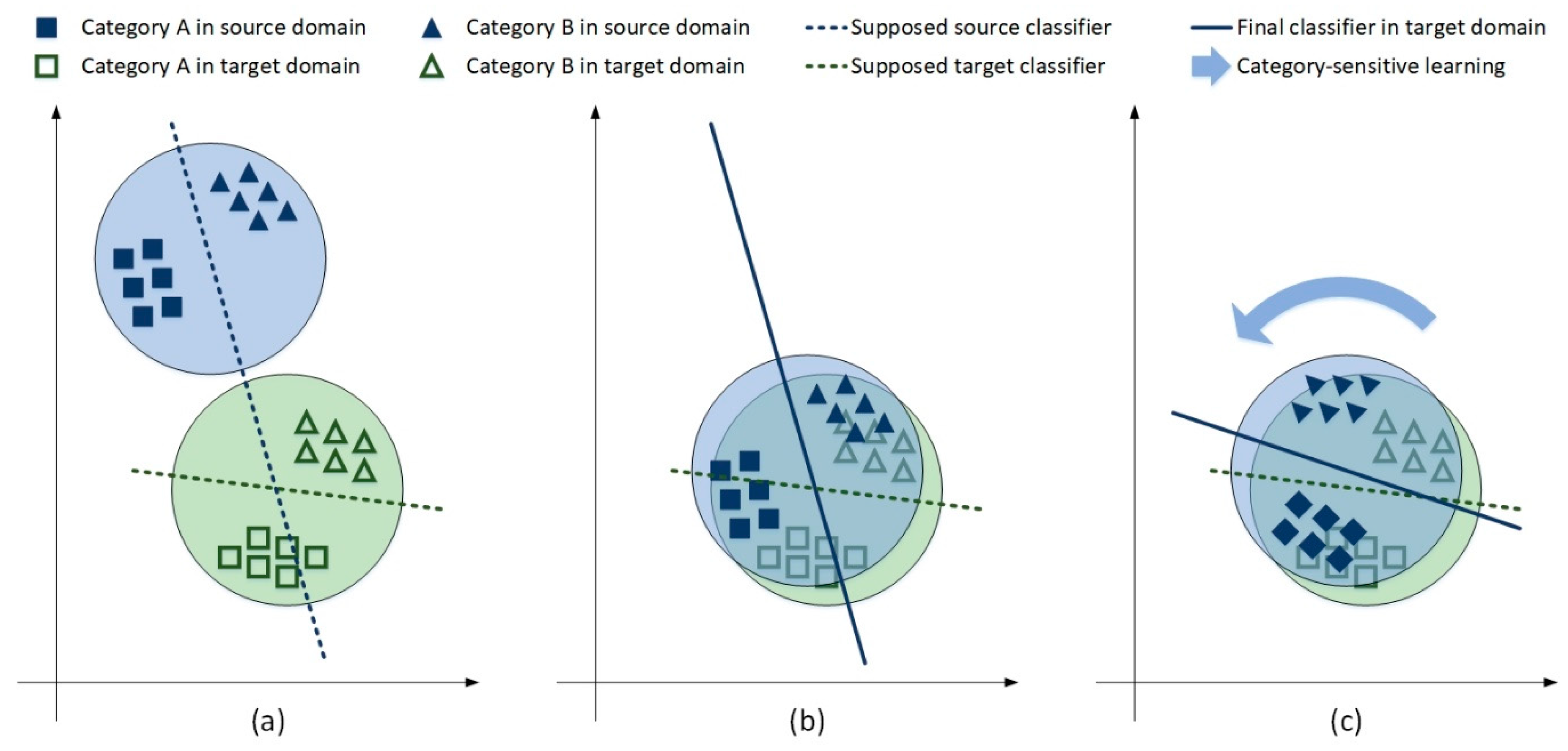
Given source aerial images with corresponding pre-labeled reference land cover maps and target aerial images without reference, the primary goal is to learn a model that can precisely perform pixel-level classification and produce correct land cover maps for the target aerial images. In our research, we hypothesize two classification models that can make correct predictions on the source and target images respectively, as illustrated in
Figure 1a. At this stage, it is notable that these two classifiers are unable to distinguish between two categories of samples in each other’s domain. To eliminate the domain discrepancies between these two types of data, conventional domain adaptation methods generally attempt to conduct global domain transfer for the source images and the supposed source classifier simultaneously, then regard the transferred classifier as the final one for the target domain. Practically, a final classifier learned in this way still cannot correctly separate the two categories of samples, as illustrated in
Figure 1b, where the final classifier incorrectly recognizes certain A samples as B samples. These results demonstrate that merely pursuing the marginal distribution alignment of source and target features leads to incorrect classification results in the target domain. To address this problem, our proposed CsDA attempts to apply category-sensitive learning after global domain adaptation to refine the final classifier until it can distinguish between two categories of samples in the target domain, as illustrated in
Figure 1c, where the final classifier can correctly separate the two categories of samples. These findings demonstrate that simultaneously preserving global domain consistency and category-level alignment between the source and target images can lead to better classification results in the target domain.
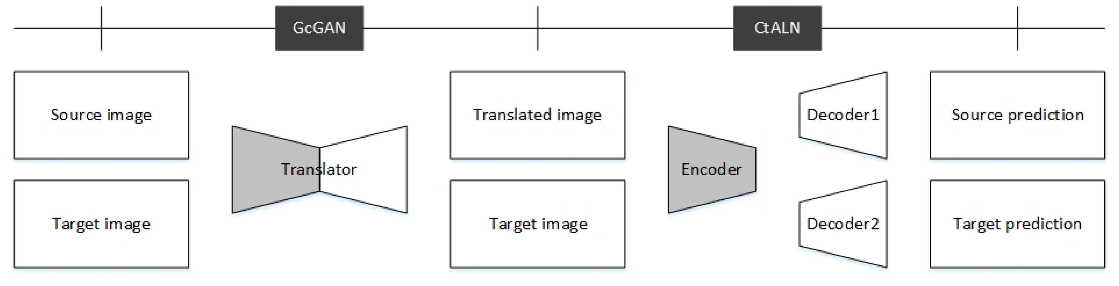
Motivated by the above observation, we propose a hybrid framework to simulate the process of our proposed CsDA, which consists of one encoder , one translator , and two decoders, and . The encoder aims to extract features separately from the source and target images, then the translator aims to translate the source features to the target domain while keeping the target features in the target domain. Finally, the decoders aim to classify the translated and target features produced by the translator, achieving land cover mapping simultaneously for the source and target images. To enable effective learning of this framework, we introduce three discriminators as adversaries. Two of them are global domain discriminators and , which both mainly aim to judge whether the translated and target features are distributed in the same domain, while the remaining one is a category-level discriminator , that mainly aims to judge whether the category distributions in the source and target predictions are aligned.
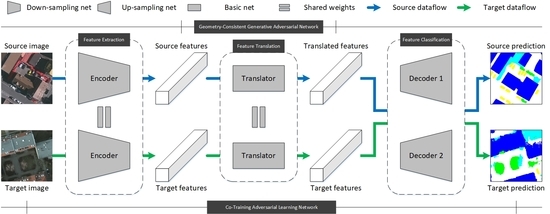
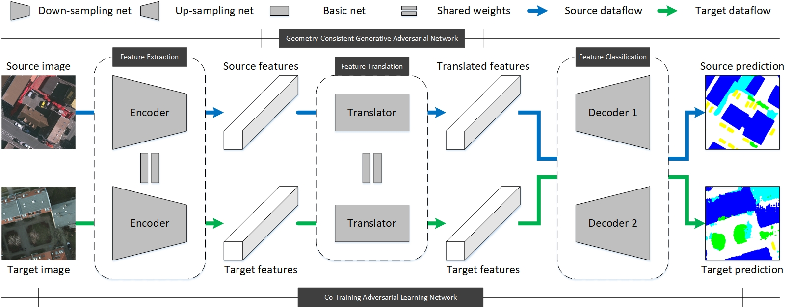
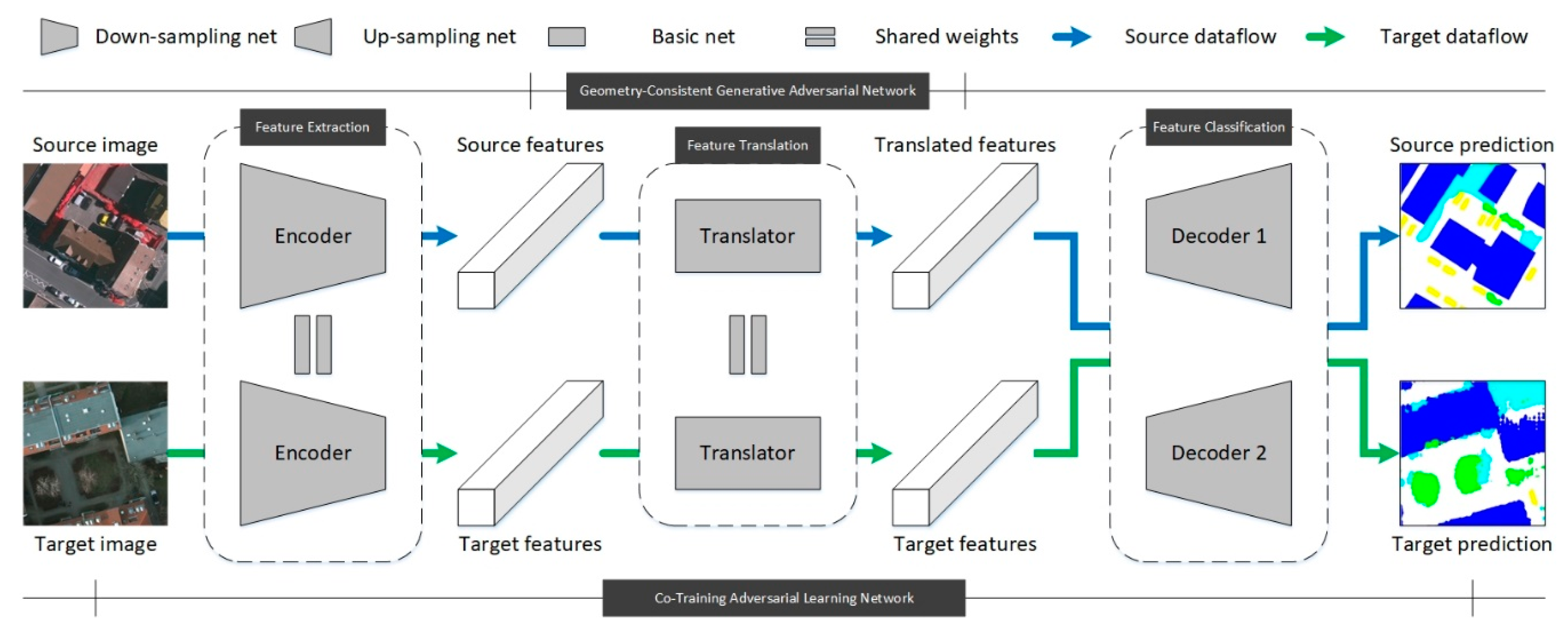
3.2. Framework Architecture
Our proposed CsDA is driven by a hybrid framework that is specifically designed as shown in
Figure 2. The framework contains three main parts, namely, feature extraction, feature translation and feature classification respectively. And there is one encoder, one translator, and two different decoders. These four neural networks make up two primary modules: GcGAN and CtALN. As the inputs of the framework, a couple of source and target images are forwarded to the same encoder and translator respectively, being processed as the translated and target features. Thereafter, these two features are simultaneously forwarded to the two decoders, and source and target predictions will serve as the final outputs. The detailed mechanisms of our GcGAN and CtALN modules are introduced in the following subsections.
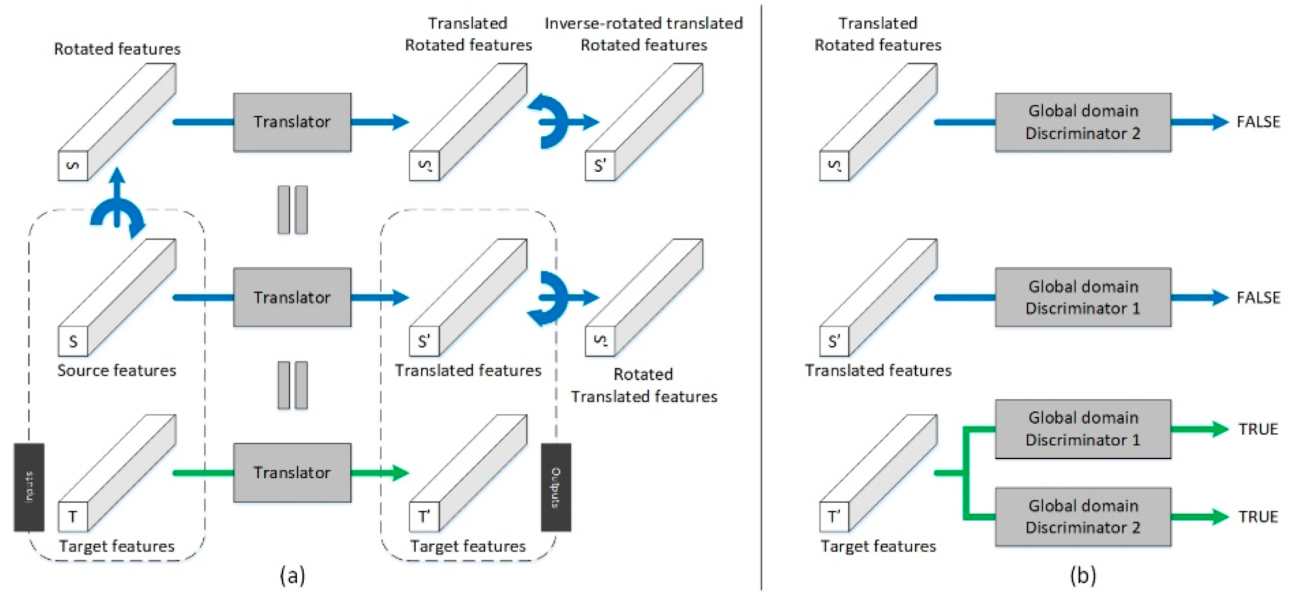
3.2.1. Geometry-Consistent Generative Adversarial Network
The primary goal of the GcGAN module is to reduce the domain discrepancies between labeled and unlabeled images and to retain the intrinsic information. This module is achieved by a translator and two global domain discriminators, as illustrated in
Figure 3.
Given a couple of source feature maps
and target feature maps
as the inputs, the rotated feature maps are defined as
, where
is a geometric rotation function for features that satisfies
. In this way, the translated rotated, translated and target feature maps can be defined as
,
and
. To enable effective learning of the translator, two discriminators are introduced to judge whether the translated rotated and translated feature maps belong to the target domain. As the adversaries of the translator, these two discriminators try to identify the target features as real features, while identifying the translated rotated and translated features as fake features, as expressed in Equations (3) and (4):
where,
and
are matrices with Boolean values of 1 and 0 respectively, which denote real and fake images pixels identified by the two discriminators. In addition, the rotation-invariant constraints can be formulated shown in as Equations (5) and (6), and the identity constraint in the target domain can be formulated as shown in Equation (7):
In this module, when training, the two global domain discriminators and the rotation-invariant constraints will simultaneously facilitate updating of the translator until it can correctly translate the source features into the target domain. When testing, however, only the translator is utilized to retain the target features in the target domain.
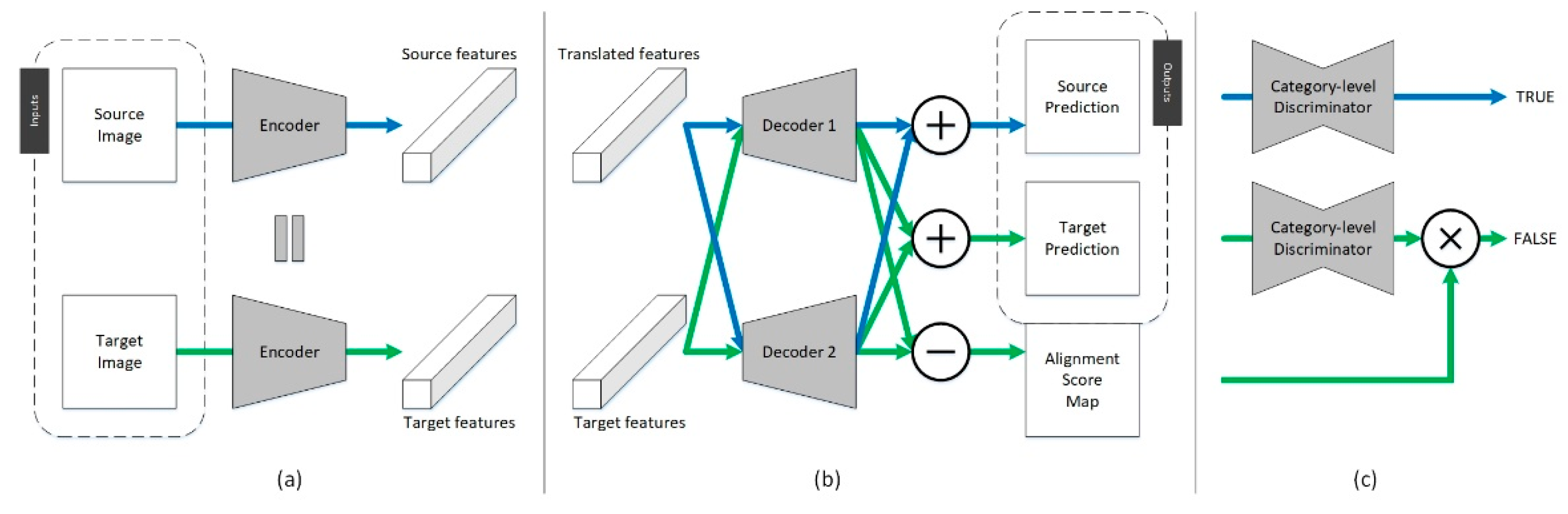
3.2.2. Co-Training Adversarial Learning Network
The primary goal of the CtALN module is to distill knowledge from the source domain and to transfer it to the target domain, by conducting a supervised and an unsupervised semantic labeling simultaneously on the labeled and unlabeled datasets. This module is achieved by an encoder, two decoders, and a category-level discriminator, as illustrated in
Figure 4.
Taking a couple of source image
and target image
as the inputs of the feature extraction part, the source and target feature maps are defined as
and
, which are the inputs of the translator in the GcGAN module. Thereafter, taking the outputs of the GcGAN as the inputs of the feature classification part, the two decoders produce a source prediction map, a target prediction map and an alignment score map, which can be defined as shown in Equations (8)–(10):
where,
is a distance metric to measure the element-wise discrepancy between two prediction maps, and it is chosen here to be the cosine distance. Specific to the pixel level, the alignment score map is defined as shown in Equation (11):
where,
is the alignment score of the pixel located at
, while
and
are two one-dimensional vectors located at
. If the angle between these two vectors is close to 0, the pixel score will be close to 0, which means that the two decoders will make similar predictions for this pixel. Meanwhile, if the angle is close to
, the pixel score will be close to 1, which means that the two decoders will make different predictions for this pixel. To enable effective learning of these two decoders, a discriminator is introduced to explore the category-level alignment degree between the source and target prediction maps. As the adversary of the two decoders, the discriminator tries to identify source predictions as real predictions, and unaligned parts of the target predictions as fake predictions, as expressed in Equation (12):
where,
represents element-wise multiplication. In addition, the co-training constraint between the weights of the two decoders is formulated as shown in Equation (13), and with the reference land cover maps
in the source domain, the supervised labeling constraint can be formulated as shown in Equation (14):
In this module, when training, the category-level discriminator and supervised constraint will simultaneously facilitate updating of all the networks until they can make correct predictions for the source images, while making similar predictions for the target images. When testing, however, only the encoder and two decoders are utilized to extract and classify features and then achieve land cover mapping in the target domain.
3.3. Loss Function
We propose a novel loss function comprised of six types of terms: (1) global domain adversarial loss to match the marginal distributions of the source and target features, (2) rotation-invariance loss to represent the geometry-consistency of the source features with and without rotation, (3) identity loss to encourage the translator to be the identity mapping for all the features in the target domain, (4) category-level adversarial loss to match the category-level distributions of the source and target features, (5) co-training loss to represent the divergence of the weights of the two diverse decoders and (6) labeling loss to evaluate whether all the networks are trained well for supervised land cover mapping on labeled images.
3.3.1. Global Domain Adversarial Loss
As the key loss of the GcGAN, global domain adversarial loss is a type of basic adversarial loss proposed by Goodfellow et al. [
37]. This type of loss increases the ability of the generator to fool the discriminator, hindering it from distinguishing translated features from target features in the same domain. In our GcGAN module, here we apply two adversarial losses, for the translated and translated rotated features, as expressed in Equations (15) and (16), respectively:
where,
tries to translate the source and rotated features to the target domain, making them similar to the target features, while
and
try to separate them, as shown in Equations (3) and (4). Therefore, the translator aims to minimize these losses against the discriminators that aim to maximize them, as in
and
.
3.3.2. Rotation-Invariance Loss
Rotation-invariance loss is a special type of reconstruction loss that relies on geometric rotation function, which was first proposed by Benaim et al. [
40]. Specifically, for the rotation invariance of land cover objects in aerial images, this loss is set to enforce two couples of translated features to be similar at the pixel level. Concretized from Equations (5) and (6), the rotation-invariance loss can be expressed as shown in Equation (17):
where,
is the L1 distance loss. Minimizing this loss makes our translator sensitive to land cover categories, improving the generalization ability of our framework.
3.3.3. Identity Loss
As a result of the powerful expression capabilities of deep neural networks, our solution for the translation from the source domain to the target domain is generally stochastic and not unique. To stabilize the translator, here we apply identity loss to ensure that the translator would keep the target features as invariant. Since its introduction by Taigman et al. [
48], this type of loss has been widely utilized in unsupervised domain adaptation, such as DistanceGAN [
40] and CycleGAN [
18]. Concretized from Equation (7), identity loss can be expressed as shown in Equation (18):
where,
is the L1 distance loss. Minimizing this loss decreases the randomness of our translator, providing a positive direction for the convergence procedure.
3.3.4. Category-Level Adversarial Loss
As the key loss of the CtALN, category-level adversarial loss is a type of basic adversarial loss, which is similar to the global domain adversarial loss described in
Section 3.3.1. Derived from the self-adaptive adversarial loss introduced by Luo et al. [
17], category-level adversarial loss aims to increase the ability of the generator to fool the discriminator, hindering it from distinguishing the unaligned parts of the target prediction from the source prediction, as expressed in Equation (19):
where,
and
denote
and
respectively. To simplify the expression of this loss, we use
to represent the entire process of the framework, which satisfies
.
is the adaptive weight for the element-wise discrepancy between two predictions and
is a small bias used to stabilize the training process. In this loss function,
tries to produce correct predictions for target images without reference, while
tries to separate them based on source predictions, as shown in Equation (12). Therefore, the generator aims to minimize this loss against the discriminator that aims to maximize it, as in
.
3.3.5. Co-Training Loss
As first proposed by Zhou et al. [
49], co-training loss is a constraint rather than a specific loss function. To provide two diverse perspectives for one semantic labeling task, the two decoders are suggested to have entirely diverse parameters. Based on this mechanism, we apply co-training loss here to enforce the divergence of the weights of all the convolutional layers in our two decoders by minimizing their cosine similarity. Concretized from Equation (13), the co-training loss can be expressed as shown in Equation (20):
where,
denotes the operation used to collect all the weights of a network, then reshape and concatenate them into a one-dimensional vector.
means the norm of a vector. Minimizing this loss makes our two decoders orthogonal vectorially, leading to more precise predictions for target images.
3.3.6. Labeling Loss
Labeling loss is an essential type of multi-class cross entropy loss that is often used in supervised semantic labeling tasks with FCN [
9]. With source images and their reference land cover maps, we employ a LogSoftmax function as our labeling loss here to make the source predictions be near their reference labels at the pixel level. Concretized from Equation (14), the labeling loss can be expressed as shown in Equation (21):
where,
means the prediction probability of category
of the pixel located at
, while
means the reference probability of category
of the pixel located at
, where if this pixel belongs to category
,
, otherwise
. Minimizing this loss makes our framework achieve supervised land cover mapping on source images.
In general, the full objective of our GcGAN module is an integration of the two global domain adversarial losses, the rotation-invariance loss and the identity loss, as formulated in Equation (22). Meanwhile, the full objective of our CtALN module is an integration of the category-level adversarial loss, the co-training loss and the labeling loss, as formulated in Equation (23):
where,
denotes the relative importance for each of these six loss functions. Therefore, the overall objective of our framework can be formulated as shown in Equation (24):
Therefore, the main solutions for this overall objective can be expressed as shown in Equations (25) and (26):
Guided by certain reference land cover maps for source aerial images, we train all the networks on the same timeline. When testing, however, only the trained encoder, translator, and decoders are used for land cover mapping on unlabeled aerial images in the target domain.
3.4. Implementation
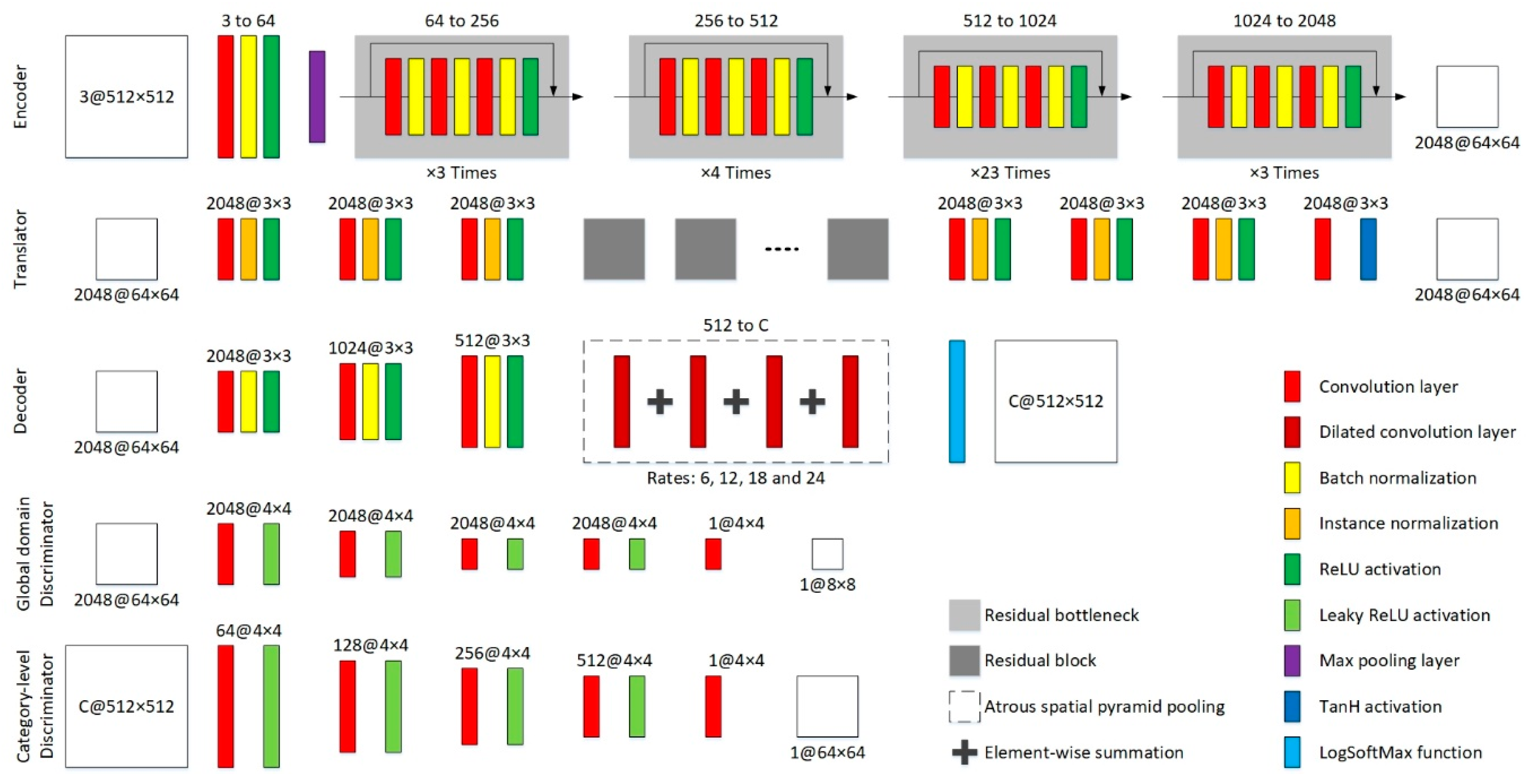
3.4.1. Network Architecture
Our proposed CsDA is driven by seven neural networks, which are one encoder, one translator, two decoders, two global domain discriminators and, one category-level discriminator respectively. The architectures of them are illustrated in
Figure 5. Taking DeepLab [
12] with ResNet 101 [
50] as the backbone, the encoder consists of a convolutional block, a max-pooling layer, and multiple residual bottlenecks. This network conducts eightfold down-sampling on the input image patches, producing feature maps with dimensions of
. The translator, derived from the generator in CycleGAN [
18], is composed of six residual blocks without down- or up-sampling operation, and the decoders are both composed of three up-sampling convolutional blocks and an atrous spatial pyramid pooling (ASPP) block, followed by a LogSoftMax layer. For our three discriminators, we adopt a Markovian discrimination strategy [
51] to model only the high-frequency structures of features or images, since the couple of input features or images of these discriminators are unpaired. Therefore, similar to the discriminator in pixel-to-pixel GAN [
39], our three discriminators are all PatchGANs, which conduct eightfold down-sampling on the input features or images. In addition, we suggest utilizing the pre-trained model on ImageNet [
52] as the backbone of the encoder. For the other six networks, all the weights and biases of their layers are initialized using the strategy of Xavier [
53].
3.4.2. Training Detail
For all the experiments, our primary goal is to obtain well-trained models through the training process that minimizes the overall objective
. In our research, according to the implementation in GcGAN [
41], we set
,
and
to 0.001, 0.02 and 0.01, respectively, in Equation (22). On the other hand, according to the implementation in CLAN [
27], we set
,
and
to 0.001, 0.01 and 1 respectively, in Equation (23), and set
and
to 10 and 0.4 respectively, in Equation (19). To stabilize the training process, we choose the least-squares loss specifically for
and
, instead of the negative log likelihood loss in traditional GANs [
37,
38].
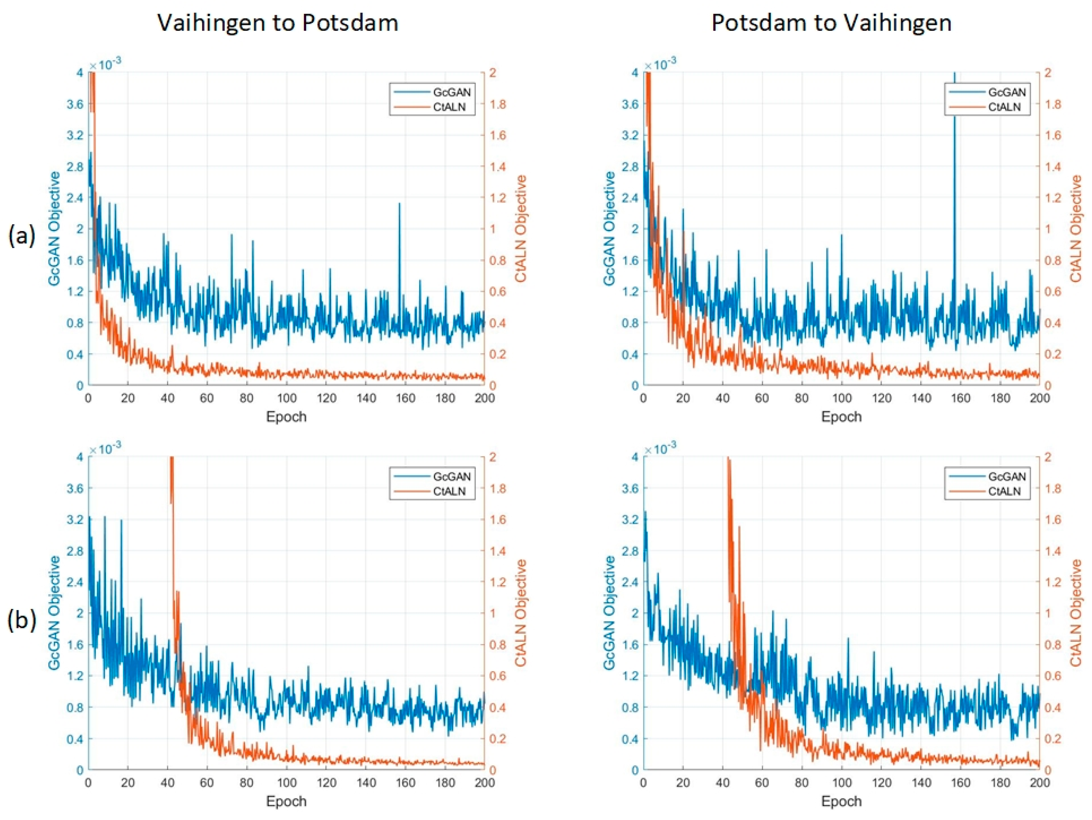
Given the complexity of the hybrid framework, we utilize a hierarchical learning strategy in the optimization procedure. For the first one fifth of the epochs, we train the GcGAN module using only the objective
. During this process, only the translator is being updated until it can translate the source features to the target domain effectively. Thereafter, for the last four fifths of the epochs, we train both the CtALN and GcGAN modules alternately with the objectives
and
. For the backward propagation in one epoch, we firstly update the encoder, the translator, and the two decoders once, and then update only the translator a second time. The overview of the training process for our hybrid framework is presented in
Table 2.
4. Experiments
4.1. Datasets Description
Vaihingen dataset [
54]: This benchmark dataset consists of 33 aerial images collected over a 1.38 square kilometer area of the city of Vaihingen with a spatial resolution of 0.09 m/pixel. On average, these aerial images all have dimensions of approximately
, and each of them has three bands corresponding to the near infrared (NIR), red (R) and green (G) bands delivered by the camera. Notably, only 16 of them are manually labeled with land cover maps, where the pixels are classified into six land cover categories, which are impervious surfaces (Imp. surf.), buildings (Build.), low vegetation (Low veg.), trees (Tree), cars (Car), and clutter/background (Clu./Back.), respectively.
Potsdam dataset [
55]: This benchmark dataset consists of 38 aerial images collected over a 3.42 square kilometers area of the city of Potsdam with a spatial resolution of 0.05 m/pixel. These aerial images all have dimensions of
, and each of them has four bands corresponding to the infrared (IR), red (R), green (G) and blue (B) bands. Only 24 of them are manually labeled with land cover maps, according to the same classification rules as for the Vaihingen dataset.
For these two datasets, certain basic information including the spatial resolution, mean value of each band, number of labeled/unlabeled images, and proportions of different categories, is computed and summarized in
Table 3. It is notable that the different land cover categories are proportionally unbalanced, for example, cars and clutter/background are much less represented than others.
4.2. Methods Comparison
In this research, the performance of our proposed CsDA is compared with those of several state-of-the-art methods. As the pioneer work applying adversarial learning for unsupervised domain adaptation, CycleGAN [
18] is set to be the baseline method in our comparison. As the first work applying domain adaptation for semantic segmentation, FCNwild [
36] is the representative of pixel-level methods. CyCADA [
23] and BDL [
24] are the representatives of methods based on pixel- and feature-constraints, while CBST [
26] and CLAN [
27] are the representatives of methods considering category-level constraints. In addition, Benjdira et al. [
14] recently cascaded a CycleGAN and a semantic segmentation model and proposed a stepwise method of achieving unsupervised domain adaptation for semantic segmentation of aerial images. As the latest land cover mapping approach, it is utilized in our comparison as well. For all the competitors, we use a same pre-trained DeepLab model with ResNet 101 as their semantic labeling models, and all the experiments are performed for the same tasks on the same datasets.
4.3. Evaluation Metrics
To prove the validity and effectiveness of the cross-domain land cover mapping methods, the following four indices are used to evaluate the accuracy of the experimental results.
Overall Accuracy (OA): The overall accuracy is generally used to assess the total capability of land cover mapping models, as expressed in Equation (27):
where,
,
,
, and
are the numbers of true positive, true negative, false positive, and false negative pixels respectively, and
indicates that the index refers to the
th category of ground objects.
Mean F1 Score (mF1): This statistical magnitude is the harmonic average of the precision and recall rates. It is generally used to evaluate neural network models, as expressed in Equation (28):
Intersection over Union (IoU) and Mean IoU (mIoU): These two indices are standard measures of classification-based methods. IoU calculates the ratio between the pixel numbers in the intersection and union of the prediction and reference for each category, as expressed in Equation (29):
Therefore, mIoU can be calculated as expressed in Equation (30):
It is notable that OA and mF1 mainly focus on the overall pixel accuracy, while IoU and mIoU mainly concentrate on the category-level pixel accuracy. For these four indices, large values suggest better results.
4.4. Experimental Setup
To verify the accuracy and efficiency of this method, we conduct two experiments between the aforementioned two benchmark datasets. For the Vaihingen dataset, we use the NIR, R and G bands as the pseudo RGB aerial images, while for the Potsdam dataset, we use the R, G and B bands as the true RGB aerial images. Before the experiments, it is essential to conduct certain pre-processing on these two datasets as follows:
Unlike objects in common natural images, certain ground objects in aerial images have constant scale ranges [
56]. Therefore, we make the two datasets consistent in scale, by resampling the Potsdam dataset to obtain a spatial resolution similar to that of the Vaihingen dataset.
To accelerate the convergence of the weight and bias parameters in all the models, we perform mean-subtraction on all the aerial images. The mean values of each band in the two datasets are listed in
Table 3.
In the experiments, if the Vaihingen dataset is set as the source data, we take the 16 Vaihingen labeled aerial images with their land cover maps and the 14 Potsdam unlabeled aerial images as the training data, while utilizing the 24 Potsdam labeled aerial images and their references for testing and assessment. On the contrary, if the Potsdam dataset is set as the source data, the 24 Potsdam labeled aerial images with their land cover maps and the 17 Vaihingen unlabeled aerial images are taken as the training data, while the 16 Vaihingen labeled aerial images and their references are utilized for testing and assessment. In addition, all the data involved in the experiments are small image patches with dimensions of , which are randomly cut from the two datasets.
For the optimization procedure, we set 200 epochs to achieve overall convergence, and each epoch involves 960 iterations. For the encoder, translator and two decoders, we used stochastic gradient decent (SGD) with a momentum [
57] of 0.9 as the optimizer, where the initial learning rate is set to
and progressively decayed to 0 by a poly learning rate policy. Meanwhile, for all the discriminators, we use Adaptive Moment Estimation (Adam) [
58] as the optimizer, where the initial learning rate is set to
and linearly decayed to 0. The decay rates for the moment estimates are 0.9 and 0.999 respectively, and the epsilon is
.
In the present research, our proposed CsDA is implemented in a PyTorch environment, which offers an effective programming interface written in Python. The experiments are performed on a computer with Intel Core i7, 32GB RAM, and NVIDIA GTX 1080 GPU. When training, the times for the partial epoch and entire epoch are 335 and 1210 seconds, respectively. With 200 epochs, the entire time for the training process of one experiment is approximately 58 hours. On the other hand, when testing, the time for one target aerial image patch with dimensions of is just 0.19 second.
4.5. Result Presentation
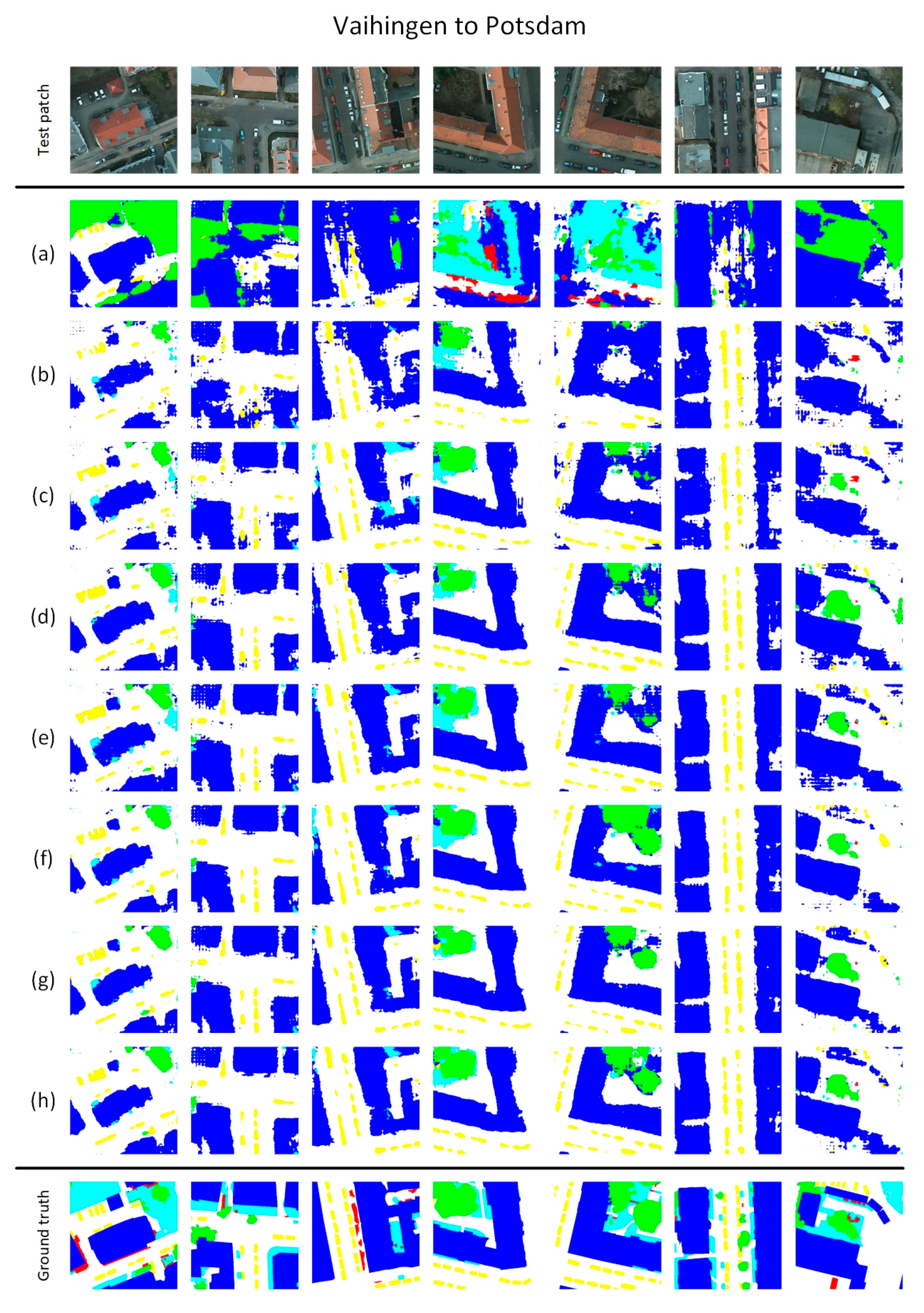
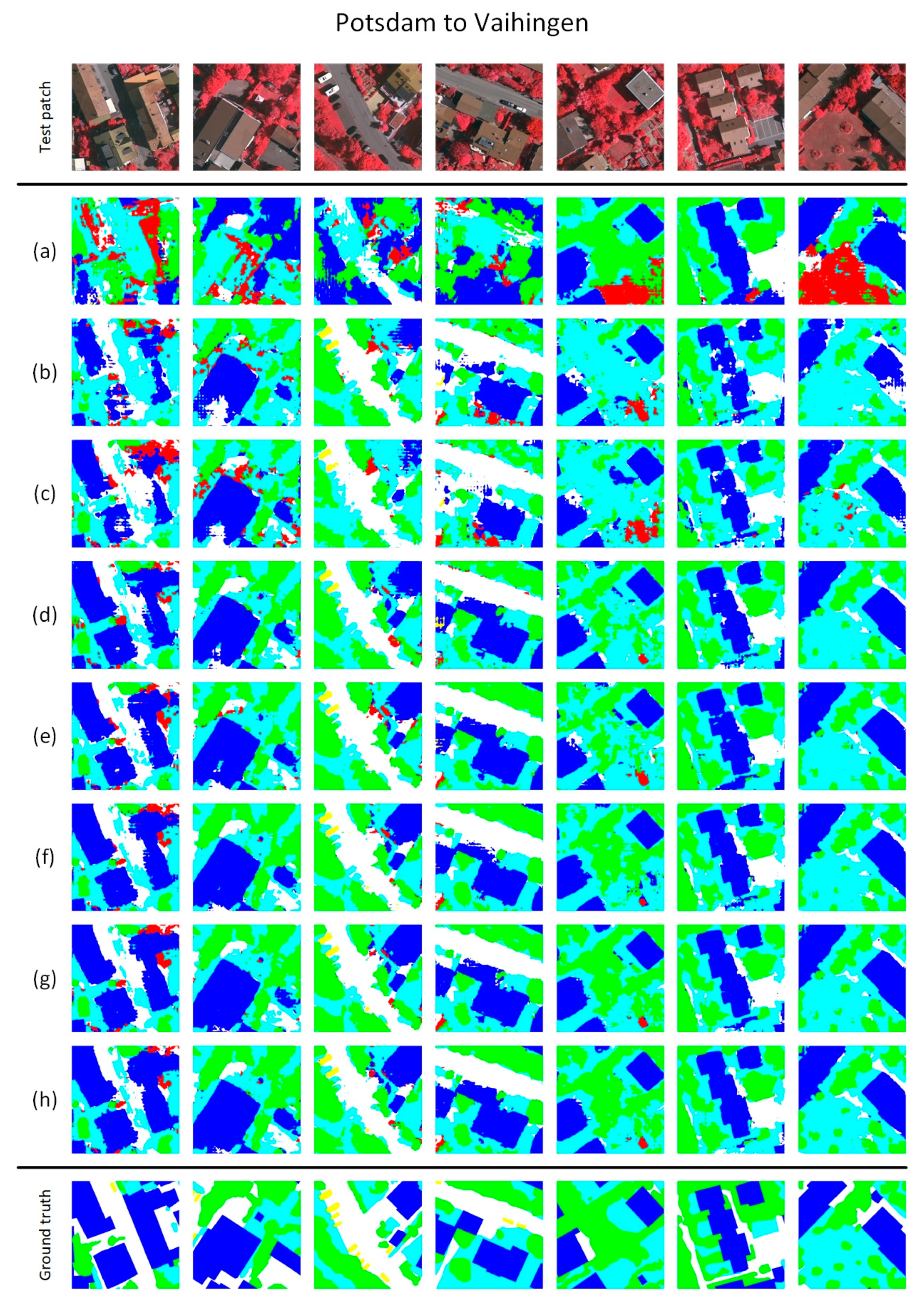
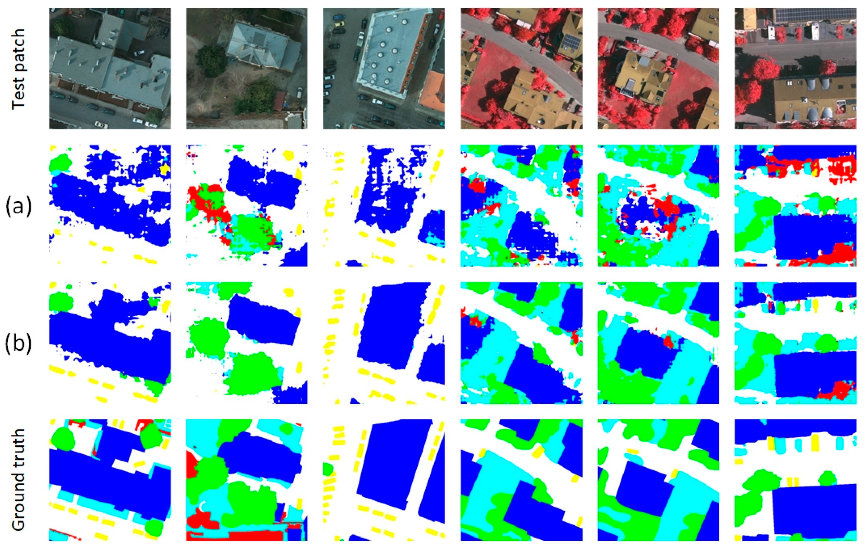
For the two experiments: from Vaihingen to Potsdam and from Potsdam to Vaihingen, the land cover mapping results obtained using our proposed CsDA and all the competitors are presented in
Figure 6 and
Figure 7, where the white, blue, cyan, green, yellow, and red regions respectively indicate the categories of impervious surfaces, buildings, low vegetation, trees, cars, and clutter/background. As can be seen, the testing results of the Vaihingen dataset are visually better than those of the Potsdam dataset, because, as guidance for each other, the Potsdam land cover maps are annotated more elaborately and precisely than the Vaihingen land cover maps.
Since CycleGAN is merely an unsupervised domain adaptation method that is agnostic to any particular task, its testing results are full of errors and uncertainties, as shown in
Figure 6a and
Figure 7a. As the representatives of pixel-level methods, FCNwild and Benjdira’s methods give approximate positions for the land cover categories but ambiguous outlines. Due to the weak constraints at the pixel level, their testing results remain unsatisfactory for real applications, as shown in
Figure 6b,c, or
Figure 7b,c. With the addition of feature-level constraints, CyCADA and BDL yield better results than the pixel-level methods. Especially in terms of ground object distributions, feature-level constraints can facilitate the models encouraging individuals to be distinctly isolated from one another. However, certain boundaries between different categories of ground objects remain rough, while certain predictions of large-scale ground objects involve many holes, as shown in
Figure 6d,e, or
Figure 7d,e. By considering category-level constraints, CBST and CLAN are able to achieve more precise and clearer predictions, which are largely free from noise, as shown in
Figure 6f,g, or
Figure 7f,g. These findings confirm that, for cross-domain land cover mapping, category-level constraints provide superior guidance compared to the other constraints. As shown in
Figure 6h and
Figure 7h, our proposed CsDA, which considers multiple constraints and geometry consistency, achieved the best testing results, where the contours of the predicted ground objects are more accurate and smoother than those obtained using CBST and CLAN.
With the testing results obtained using our proposed CsDA and other comparative methods, the evaluation metrics OA, mF1, IoU and mIoU, and the processing rate for these two cross-domain land cover mapping experiments are computed and summarized in
Table 4 and
Table 5. Compared with other state-of-the-art methods, although our proposed CsDA has a slower processing rate of 0.19 second per image patch, it achieves the highest OA, mF1, and mIoU values of 60.4%, 52.8% and 42.3% in the experiment from Vaihingen to Potsdam and 65.3%, 54.5% and 44.9% in the experiment from Potsdam to Vaihingen, respectively.


