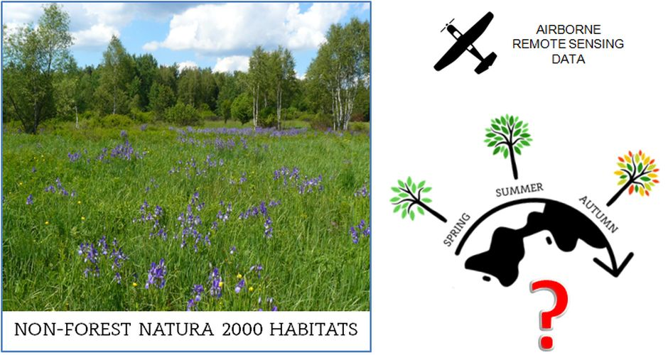
Mapping Succession in Non-Forest Habitats by Means of Remote Sensing: Is the Data Acquisition Time Critical for Species Discrimination?

Abstract

The process of secondary succession is one of the most significant threats to non-forest (natural and semi-natural open) Natura 2000 habitats in Poland; shrub and tree encroachment taking place on abandoned, low productive agricultural areas, historically used as pastures or meadows, leads to changes to the composition of species and biodiversity loss, and results in landscape transformations. There is a perceived need to create a methodology for the monitoring of vegetation succession by airborne remote sensing, both from quantitative (area, volume) and qualitative (plant species) perspectives. This is likely to become a very important issue for the effective protection of natural and semi-natural habitats and to advance conservation planning. A key variable to be established when implementing a qualitative approach is the remote sensing data acquisition date, which determines the developmental stage of trees and shrubs forming the succession process. It is essential to choose the optimal date on which the spectral and geometrical characteristics of the species are as different from each other as possible. As part of the research presented here, we compare classifications based on remote sensing data acquired during three different parts of the growing season (spring, summer and autumn) for five study areas. The remote sensing data used include high-resolution hyperspectral imagery and LiDAR (Light Detection and Ranging) data acquired simultaneously from a common aerial platform. Classifications are done using the random forest algorithm, and the set of features to be classified is determined by a recursive feature elimination procedure. The results show that the time of remote sensing data acquisition influences the possibility of differentiating succession species. This was demonstrated by significant differences in the spatial extent of species, which ranged from 33.2% to 56.2% when comparing pairs of maps, and differences in classification accuracies, which when expressed in values of Cohen’s Kappa reached ~0.2. For most of the analysed species, the spring and autumn dates turned out to be slightly more favourable than the summer one. However, the final recommendation for the data acquisition time should take into consideration the phenological cycle of deciduous species present within the research area and the abiotic conditions.

1. Introduction

We are currently witnessing a loss of biodiversity, which has profound consequences for the natural world and for human well-being. The main causes of this loss are changes to natural habitats due to intensive agricultural production systems; construction; quarrying; the overexploitation of forests, oceans, rivers, lakes and soils; invasive alien species; pollution; and, increasingly, global climate change [1,2,3]. The preservation of natural biodiversity has been one of the priorities of environmental policy in Europe for many years [1,4]. The EU Biodiversity Strategy to 2020 is fully in line with the UN Convention on Biological Diversity, the most important global biodiversity policy dedicated to halting the loss of biodiversity and the loss of ecosystem services by 2020. The Strategy addresses nature (target 1), ecosystems and their restoration (target 2), the sustainable use of Europe’s nature, land and sea resources via agriculture, forestry and fisheries (targets 3 and 4), the problem of alien species (target 5) and the EU’s global impacts (target 6) [1]. The EU nature protection policy is based on two main legal acts: The Birds Directive and the Habitats Directive. These form the basis for the operation of the Natura 2000 network, a network of protected areas to safeguard the species and habitats of highest interest within Europe.

Each EU Member State is obliged to monitor the condition of natural habitats in Natura 2000 areas, and if a threat is found, to take measures to counteract the deterioration of habitat status. The monitoring methods currently used are based on an expert approach, which is characterised by a high level of subjectivity and is a time-consuming process. A possible alternative to this expert approach is remote sensing. As previous research studies show, it can be used to identify natural habitats [5,6,7,8,9], to map and assess their conservation status [8,10,11], and to identify their threats by monitoring invasive and expansive plants [12,13,14,15], secondary succession [16,17,18] and desiccation [19,20,21]. In order to make use of remote sensing methods for monitoring individual habitats and their threats as efficiently as possible, it is necessary to define requirements (including the most suitable dates for acquiring remote sensing data) and to identify limitations resulting from its use in various habitats. The HabitARS project is “An innovative approach supporting the monitoring of non-forest Natura 2000 habitats, using remote sensing methods”. Within its framework, actions have been taken to develop guidelines on the methodology for identifying—with the use of remote sensing techniques—natural and semi-natural open Natura 2000 habitats (i.e., alkaline fens, European dry heaths, semi-natural dry grasslands, species-rich Nardus grasslands, Molinia meadows, transition mires and quaking bogs) and the threats to them, such as desiccation, encroachment of invasive and expansive plants and succession of trees and shrubs. The last of the above-mentioned threats is the subject of the research presented here.

The process of secondary succession is one of the most significant threats to non-forest Natura 2000 habitats in Poland. These are natural habitats listed in Annex II of the Habitats Directive, which form plant communities, naturally developed (e.g., wetlands) or as a result of human activity (e.g., meadows), in which the vegetation structure does not contain woody species. Shrub and trees encroachment taking place on abandoned, poorly productive agricultural areas, historically used as pastures or hay meadows, leads to compositional changes in species (e.g., disappearance of photophilous species) and biodiversity loss (e.g., disappearance of avifauna, herpetofauna or entomofauna species, associated with open habitats), and results in landscape transformations [22,23,24]. The main factor allowing the maintenance of valuable semi-natural, open ecosystems in Poland is regular, extensive mowing or grazing. Annual mowing and harvesting of biomass as well as grazing reduce the spread of trees and shrubs. Due to cessation of use, the process of secondary succession is initiated and leads to the formation of forest and shrub communities. In Poland, during the political transformation (1989) and the resulting changes in the economy, in many regions of the country land abandonment occurred, which contributed to overgrowing with trees and shrubs of previously used agricultural plots. Currently, the decline in the use of agricultural plots initiating succession occurs to a lesser extent and is associated with demographic processes. In the case of wetland habitats, the permanent limiting moisture content is a factor limiting succession towards forest and shrub communities. In the situation of desiccation of wetlands, favourable conditions for the development of shrub communities and then of the forest are formed [25,26,27]. Depending on the habitat, different species have successive tendencies. The main succession species in non-forest habitats in Poland are Alnus glutinosa (L.) Gaertn., Betula pubescens Ehrh., Betula pendula Roth, Crataegus spp., Cornus sanguinea L., Juniperus communis L., Prunus serotina Ehrh., Pinus sylvestris L., Populus tremula L., Prunus spinosa L., Rhamnus cathartica L., Salix cinerea L. and Salix rosmarinifolia L. [28,29,30]. However, not all of these species pose the same level of threat, and some of them are more expansive than others, depending on the habitat type analysed. Information about the distribution of dominant species is therefore needed in order to plan appropriate protection measures. As the phenology of various succession species differs, the optimal date for their differentiation, and consequently the acquisition of remote sensing data, needs to be determined.

For years, many scientists throughout the world, and especially those dealing with forestry, have undertaken research work on delineating various forest types or stands e.g., [31,32,33] and tree species e.g., [34,35,36,37,38,39,40,41,42,43,44,45,46,47]. The mapping of urban tree species has also been a widely studied research topic in the last decade e.g., [48,49,50,51,52,53,54]. A wide review of studies on the classification of tree species from remotely sensed data was presented by Fassnacht et al. [55] and demonstrated that the number of studies focusing on the classification of tree species has been constantly increasing over the last four decades. In a summary of their review, Fassnacht et al. [55] found that passive optical systems, and especially hyperspectral systems, generally showed higher potential for the classification of tree species than active SAR or LiDAR (Light Detection and Ranging) sensor systems, as they enabled to obtain similar accuracies but for a higher number of tree species. In recent years, many studies have also examined the use of combination of LiDAR and hyperspectral data for identification of tree species [36,45,46,48,51,54,56]. The accuracy of tree species classification reported by different researchers varies. Depending on the date of remote sensing data acquisition, Voss and Sugumaran [40] obtained an overall accuracy of around 56–57% for seven tree species using both hyperspectral and LiDAR data, and 45–48% using only hyperspectral data. Zhang and Qiu [51] achieved a total accuracy of classification of 68.8% for 20 tree species. Alonzo et al. [52] obtained an overall classification accuracy of 79.2% for hyperspectral data analysis, 32.9% for LiDAR data classification, and 83.4% based on a fusion of both data sets. Dalponte et al. [36] also showed that the best accuracy of species classification was obtained when hyperspectral data were combined with variables obtained from LiDAR data. The information about the geometry of research objects derived from LiDAR relate to the structure of vegetation, branching and foliage [57,58], and support the delimitation of individual tree species.

Another trend in research in the field of tree species discrimination is multi-temporal data analysis. The number of studies on this topic has increased due to the free provision of LANDSAT satellite images and the launch of new satellites in the European Sentinel series e.g., [40,47,59,60,61]. The use of multi-temporal data allows researchers to take advantage of the spectral variability of individual species in different phenological periods, and thus supports the successful separation of tree species using multispectral or hyperspectral data sets (e.g., [59,61,62,63,64]). The review by Fassnacht et al. [55] mentioned above shows that the application of multi-temporal hyperspectral data with the aim of improving classification results has rarely been examined. According to these authors, multi-temporal hyperspectral data sets may only be of scientific interest at present, as the costs and effort connected with the acquisition and processing of multiple hyperspectral data sets (the ‘big data problem’) are not likely to justify the achievable gain in accuracy from a practitioner’s perspective. In terms of the practical application of hyperspectral data in monitoring the succession process in non-forest Natura 2000 habitats, it is important to determine the optimal date for acquiring remote sensing data. The optimal date is the one on which a high accuracy of delineation can be obtained for as many species as possible of succession trees and shrubs. Defining the optimal data acquisition period is therefore of key importance for the implementation of hyperspectral remote sensing data in the operational monitoring of the status of Natura 2000 natural habitats.

The objectives of this study were: (1) To analyse the impact of the remote sensing data acquisition date on the effectiveness of classification of individual species of succession trees and shrubs; and consequently (2) to indicate the most favourable date for collecting this data; and (3) to show whether the classification accuracy of a given species is dependent on the research area, and the analysed habitat.

2. Study Areas

For the study presented here, we selected five Natura 2000 sites in Poland: The Biebrza River Valley (BI), the Lucynów-Mostówka Inland Dunes (BU), the Nidziańska Refuge (NI), the Krasna Valley (KR), and the Janowskie Forest Ranges (LJ) (Figure 1).

These five research areas lie within the Special Areas of Conservation established on the basis of the Habitat Directive in order to preserve habitat types (

Table 1. Description of the Natura 2000 sites studied, including the non-forest habitat types threatened by succession of trees and shrubs.

Natura 2000 Site	Natura 2000 Code	Geographical Coordinates	Acronym	Study Area (km2)	Type of Natura 2000 Habitat Studied (code)	Promoters of Succession
Biebrza River Valley	PLH200008	53°17′10″N; 22°37′45″E	BI	37	Alkaline fens (7230)	Alnus glutinosa, Betula pubescens, Salix cinerea, Salix aurita, Salix rosmarinifolia
Lucynów-Mostówka Inland Dunes	PLH140013	52°35′34″N; 21°27′30″E	BU	7	European dry heaths (4030)	Pinus sylvestris, Betula pendula, Populus tremula, Prunus serotina
Nidziańska Refuge	PLH26003	50°32′14″N; 20°30′42″E	NI	23	Semi-natural dry grasslands and scrubland facies on calcareous substrates (Festuco-Brometalia) (6210)	Pinus sylvestris, Prunus spinosa, Rosa canina
Krasna Valley	PLH260001	50°45″N; 19°17″E	KR	41	European dry heaths (4030); species-rich Nardus grasslands on siliceous substrates in mountain areas (6230); Molinia meadows on calcareous, peaty or clayey, silt-laden soils (Molinion caeruleae) (6410)	Salix cinerea, Salix aurita, Frangula alnus, Betula pendula, Pinus sylvestris
Janowskie Forests Ranges	PLH060031	50°43″N; 22°0″E	LJ	43	European dry heaths (4030); transition mires and quaking bogs (7140)	Quercus robur, Populus tremula, Betula pendula, Betula pubescens, Pinus sylvestris

). Smaller individual study areas have been identified for investigation within the project, on the basis of non-forest habitat types threatened by the spontaneous succession of trees and shrubs. Additional selection criteria were related to the geographical distribution of Natura 2000 sites and their abiotic conditions, especially the local climate, shallow geology, types of rocks and soils, habitat humidity and types of landforms present. Another important factor considered in the selection of study areas was related to limitations on human activity: most of the areas chosen have been withdrawn from agricultural production. In particular, the shape and size of each study area differ significantly, due to the types of local habitat and their spatial distributions. They are also shaped by borders of Natura 2000 sites.

The BI study area is located in north-eastern Poland, on the North Podlasie Lowland. It occupies part of a vast plain of fen mire located in the southern part of the Biebrza ice marginal valley, near Szorce, at an altitude of about 100 m above sea level. Most of the area is covered by sedge and sedge-moss peat deposits up to 2 m thick. In the western part of the area, there are small sandy hillocks with relative altitudes not exceeding 2–3 m. Various forms of alkaline fens predominate among vegetation types, often with species of tall sedge communities and a significant share of reed rushes. Forest and shrub communities occurring in the area are dominated by Alnus glutinosa and/or Betula pubescens, and to a lesser extent Salix cinerea, Salix aurita L. and Salix rosmarinifolia (five species—promoters of succession).

The BU study area is located in central Poland, on the Mazowiecka Lowland, near Wyszków, at an altitude of approximately 110 m above sea level. In geomorphological terms, it forms part of the uppermost Bug river Holocene terrace. The substrate is mostly sandy, transformed by aeolian processes. The relative altitudes of the dune hills within the area reach 20 m. Among the vegetation, forest communities with Pinus sylvestris prevail as the dominant species in the stand, with admixtures of Betula pendula and to a lesser extent Quercus robur L., Populus tremula and various species of the genus Salix. In addition to forests, there are extensive complexes of dry heathlands, dry, sandy grasslands, permanent meadows, ruderal and segetal vegetation. In terms of Natura 2000 habitats, the most valuable elements occupying large areas are European dry heaths and inland dunes. Both natural habitats are threatened by four species of trees and shrubs inducing the process of secondary succession (promoters of succession). Species entering heathland and grassland habitats are mainly Pinus sylvestris, Betula pendula and Populus tremula, as well as an alien invasive species, Prunus serotina. Juniperus communis is a shrub species that regular occurs in the dry grassland and heathland habitats of the region.

The KR study area is located in the south-east part of Poland, in Świętokrzyskie Voivodeship, near Kielce, and include a natural, strongly bogged valley of the Krasna River and its tributaries. The area is significantly diversified in terms of its geomorphological conditions and land use. In the southern and eastern parts of the Krasna Valley, non-forest ecosystems dominate. The river in this section has a wide valley, and its gradient is small. In the northern part, forests occupy the largest area, and pine forests prevail over other types. In this part of the area, the Krasna River runs in a deeply cut riverbed and has the character of a highland river. The area is characterised by a large diversity of habitats with a wealth of plant and animal species, and is protected as a Natura 2000 site. The current research is focused on three habitats for which the encroachment of woody vegetation is defined as a threat: European dry heaths, species-rich Nardus grasslands on siliceous substrates in mountain areas (and submountain areas in continental Europe) and Molinia meadows on calcareous, peaty or clayey-silt-laden soils (Molinion caeruleae W. Koch 1926). For these three habitats, five dominant/problematic species of trees and shrubs (promoters of succession) have been identified: Salix cinerea, Salix aurita, Frangula alnus Mill., Betula pendula and Pinus sylvestris.

The LJ study area is located in the south-east part of Poland, in Podkarpackie Voivodeship, near Sandomierz. The Janowskie Forest is a compact forest area with a high degree of naturalness and low population density, with fragments of old forest stands. The main habitat values here are boggy pine forests, silver fir forests (Abies alba Mill.), transitional mires and bogs. Other valuable habitats are alder forests along a number of watercourses, sandy grasslands and dry heaths located in the western part of the area (mainly in a former military location) and meadows. The research was focused on two habitats for which the encroachment of woody vegetation is defined as a threat: European dry heaths and transition mires and quaking bogs. For these habitats, four dominant/ problematic species of trees and shrubshave been identified: Quercus robur, Populus tremula, Betula pendula (on heathlands), and Betula pubescens and Pinus sylvestris in mires and bogs.

The NI study area is located in south-eastern Poland in the Małopolska Upland. This area, includes parts of the Nida river valley, the Pińczów Hummock and the Połaniecka Basin in the southern part of the Nidziańska Basin. The research area is located within a typical agricultural region near the town of Pińczów. The landscape of the area is diverse, with a river valley of about 2–6 km in width and the Cretaceous-Tertiary Pińczów Hump. To the west of Pińczów, the hills of the Hump reach a height of more than 290 m above sea level. The orography includes natural fragments of the Nida Valley as well as the neighbouring plateau. The Nida River meanders, creating numerous oxbow lakes, and this process results in the creation of large complexes of moist and wet meadows and small swamps and marshes. Gently undulating loess plateaus are separated by ravines and dry valleys, and the limestone and gypsum hills and the slopes of ravines are covered with xerothermic grasslands [65]. The whole area is sparsely forested, with a predominance of young pine woodweeds and Robinia woods. Our research focuses on one type of habitat, namely the semi-natural dry grasslands that cover the western end of the Pińczów Hump [66]. Three woody species have been identified as promoters of succession: Pinus sylvestris, Prunus spinosa and Rosa canina L. However, the diversity of trees and shrubs colonising the xerothermic grassland is much larger; in addition to the aforementioned species, common ones are Cornus sanguinea, Rhamnus cathartica, and species of the genus Crataegus and the invasive alien species Robinia pseudoacacia L.

3. Source Data

3.1. Remote Sensing Data

Five different data sets were used in the experiment, one for each study area described above. Remote sensing data were acquired three times during the growing season of 2017, referred to here as spring (C1), summer (C2) and autumn (C3). Thus, the data set for each study area included three analogous collections of data. The only exception was the BI area which lacked autumn (C3) acquisition due to the hyperspectral sensors’ failure. This schedule was used with the aim of acquiring data characterising the vegetation at various phenological phases, thereby enabling us to determine the differences in the accuracy of species differentiation, and finally to assess which is the most favourable. All dates for data acquisition are presented in

Table 2. Dates for remote sensing data acquisition.

Research Area	Remote Sensing Data Acquisition Time
	C1 Flight Campaign (spring)	C2 Flight Campaign (summer)	C3 Flight Campaign (autumn)
BI	27 June 2017	9 August 2017	-
BU	28 May 2017	10 July 2017	9 September 2017
KR	1 June 2017	7 July 2017	27 September 2017
LJ	2 June 2017	19 July 2017	9 September 2017
NI	18 May 2017	30 July 2017	27 September 2017

.

Data collected during each flight campaign included high-resolution hyperspectral imagery and fullwave LiDAR data, acquired simultaneously from the common, specially prepared aerial platform, which was built as part of the HabitARS project by the MGGP Aero company. Acquiring both data types at the same time allowed us to avoid problems resulting from changes in vegetation cover due to plant growth, phenology and various human activities, and therefore facilitated subsequent data fusion [67]. Technical parameters characterising the sensors and both data types are shown in

Table 3. Technical parameters of the sensors used and the remote sensing data they provided.

Technical Parameters	Sensor Type
	Airborne Laser Scanner (FWF) Riegl LMS-Q680i	HySpex Hyperspectral Camera
		VNIR-1800	SWIR-384
Flight Altitude AGL (m)	500
Point density (points/m2)	7	-	-
Spatial resolution (m)	-	0.5	1
Spectral resolution	1.55 µm	430 bands encompassing 0.4–2.4 µm spectral range
Spectral sampling (nm)	-	3.26	5.45
FOV max (degrees)	60	34	32
Overlap (%)	62.7	30	30
Overlap width (m)	855	450	450

.

In addition to the phenological phase, the specific weather conditions also influence the vegetation growth (both analysed and background) and the state of its surroundings (e.g., the soil). These properties determine the character of the acquired remote sensing data, and therefore affect the possibility of differentiating species based on their use.

In 2017, weather conditions in Poland were characterised by strong variability, and included the occurrence of numerous extreme phenomena (local floods in May, and severe heat waves, storms, extreme rainfalls and local whirlwinds in summer). In general, 2017 was warmer and more humid than the average conditions between 1971 and 2000. The air temperature was higher by about 1–1.5 °C, and precipitation was about 120–160% of the average level between 1971 and 2000 [68]. Spring and summer were particularly warm, and were hotter by about 1 °C–1.5 °C and 1.5 °C–2.5 °C, respectively. The total rainfall was especially high (150–300% of the average between 1971 and 2000) in north-eastern, eastern (BI and BU research areas), central and south-central parts of Poland in March and April and in September. From May to July, rainfall reached only 50–70% of the norm in south-central part of Poland (KR, LJ and NI research areas). These weather conditions contributed to a small increase in the speed of the vegetation growth, especially in spring.

3.2. Field Data

The aim of collecting the field data was to create reference sets for the classification of the tree and shrub species present in each research area. Field measurements were made for each study area in 2017 at the peak of the growing season, as species recognition is not problematic at this time.

The collected data included both species perceived as succession and others present in the study areas. We decided to implement classification—method in which every pixel of an image is assigned to one of the predefined classes (described in detail in 4.6)—rather than detection-procedure enabling to determine which pixels of an image are similar to the reference spectra—is a method of distinguishing between species. Therefore, reference spectra for other species were necessary to determine the spatial extent of species forming the succession process.

Geolocation of each spatially isolated specimen — in the future to be used in order to select the reference pixels of remote sensing data forming the reference polygons — was determined using a GPS Mobile Mapper 120 with a real-time differentially corrected global positioning system (DGPS) and a measurement accuracy of up to 0.2 m. In addition to the location and species identification, all measured objects were also characterised by other attributes, e.g., the object’s height, crown density, crown radius, level of discolouration, level of defoliation and neighbouring vegetation type. These descriptive attributes were later used in the process of creating reference polygons (described in detail in 4.4). The field data were collected in different parts of the research areas, thus ensuring diversity in respect to key parameters characterising the research objects, such as their heights or crown radii. This approach guaranteed the diversity of both future training and validation sets, enabling us to produce accurate classifications.

4. Methodology

4.1. Overview

The methodology of the experiment was based on a combination of high-resolution aerial remote sensing data and the use of a machine learning algorithm, and included the processing of each collection of remote sensing and field data according to the steps outlined in Figure 2. At the end of this work, the results obtained for each research area were examined in order to draw conclusions on the most favourable collection (data acquisition time).

The processing scheme started with a feature extraction step in which the pre-processed remote sensing data (hyperspectral true-ortho mosaic and LiDAR data) were used in order to derive useful, informative products (described in 4.2 and 4.3). At the same time, DGPS field measurements were also transformed into reference polygons using a semi-automatic algorithm developed by the authors and remote sensing data (described in 4.4). In the next step, a feature selection algorithm was applied to the obtained remote sensing products and reference polygons in order to determine the optimal set of features to be used at the classification stage (described in detail in 4.6). Using the image resulting from the classification step and the product of delineating the succession in an area (described in 4.7), the classification image was postprocessed by limiting the results to the extent of the trees and shrubs. In the next step, the accuracy of the product was assessed by combining the validation polygons with the obtained classification image, and the accuracy report was then analysed in parallel with species separability graphs, created using a t-distributed stochastic neighbour embedding (t-SNE) algorithm [69] (described in 4.5 and 4.8).

4.2. Hyperspectral Data Processing

Before the hyperspectral imagery in the experiment could be used, the data needed to be pre-processed. Raw images were first subjected to radiometric calibration using Hyspex RAD software [70]. Georeferencing and orthorectification were then applied using PARGE software [71], based on the trajectory and attitude of the plane recorded during the flight and DSM derived from simultaneously acquired LiDAR data. Next, ATCOR4 software ReSe Applications GmbH, [72] was used to carry out an atmospheric correction, the accuracy of which was controlled using field spectrometer measurements. Finally, mosaics were created from single corrected images. Data acquired for all research areas were pre-processed using the same procedures to assure their comparability.

The pre-processed data obtained from the data provider in the form of true-ortho mosaics were then used in the feature extraction step. Minimum noise transform (MNF) products [73] were calculated based on all spectral bands, and those that were characterised by low levels of noise and high information content were chosen, reducing the dimensionality of the dataset to about 15–20 components. Specific spectral bands were also used to compute a set of 65 vegetation indices, including the following vegetation categories: Broadband greenness, narrowband greenness, canopy water content, canopy nitrogen, dry or senescent carbon, leaf pigments and light use efficiency. Both feature extraction methods have been shown to be highly effective in research studies of species differentiation [55,74,75,76,77].

4.3. LiDAR Data Processing

The classifications carried out in this experiment were not only based on the hyperspectral data, but also on some additional raster layers derived from LiDAR data (

Table 4. Features derived from LiDAR (light detection and ranging) data. VEG: vegetation class; GRD: ground class; ALL: both of these classes; IQR: interquartile range of height; DTM and DSM: raster layers.

Feature Type	Statistics Generated/Description	ALS Classes
DTM	SigmaZ, slope, exposition, TPI	GRD
DSM	SigmaZ, slope, exposition	ALL
nDSM	Min, max, mean, variance, median, range, RMS, Percentiles: 5, 10, 25, 75, 90, 95	ALL, VEG
Amplitude	Min, max, mean, variance, median, range, RMS	ALL, GRD, VEG
Echo ratio	Min, max, mean, variance, median, range, RMS	ALL, GRD, VEG
Point density	Number of pts/m2	ALL, GRD, VEG
Total vegetation density	Ratio of vegetation to ground points	-
Vegetation cover	Ratio of vegetation to all points	-
IQR (interquartile range of height)	Range between quantiles 0.75 and 0.25	-

). These features were derived from point clouds, which at the beginning were classified into three classes: Ground (classified using TerraSolid software with Axelsson’s algorithm [78]), vegetation and unclassified (including all points that were not ground or vegetation). Features were then calculated from the point clouds and rasterised with OPALS software [79].

The features derived from LiDAR data could be divided into three groups. The first group of products included features derived from two raster layers (DTM and DSM): The slope, exposition, roughness (sigmaZ) and one additional feature (topographic position index) calculated from the DTM only. The second group of features was derived directly from the point clouds, and consisted of the statistical values of the normalised height of the points, the amplitude of each echo (from full-wave signal decomposition using Riegl’s software), the geometrically based echo ratio parameter [80] and a simple point density. The features in the second group were derived in a few variants: from points in the vegetation class (VEG), from points in the ground class (GRD), or from points in both of these classes (ALL), according to the idea underlying BCAL software [81]. The third group of features was directly connected with the vertical distribution of points, and contained three point-based indices: total vegetation density, vegetation cover and interquartile range of height (IQR) [82].

4.4. Reference Data Preparation

The reference polygons were created using a semi-automatic algorithm developed by the authors. The procedure started with the reclassification of an nDSM in order to separate high objects or groups of high objects. High anthropogenic objects were then excluded using an NDVI index raster, leaving only vegetation. In the next step, the layer obtained in this way was combined with botanical field data, which enabled us to determine the spatial relationship between each point (field measurement) and tree/shrub objects present nearby. In the final step, the obtained tree and shrub reference objects were subjected to pixel-level analysis. The spatial extent of each polygon was limited in order to remove the boundary and mixed pixels, and therefore to create pure spectral signatures.

For all three collections of remote sensing data, reference sets were generated separately from the same set of field measurements. This was necessary, because of phenologically induced changes in vegetation, and consequently differences in the outlines of the research objects in the airborne data. As a consequence of these phenologically induced changes, a different number of reference polygons was created for each of the three data collections for a given area. These minor differences arose from the fact that small trees and shrubs (approx. 1 m in crown diameter) were not fully formed in the data because of their size, and as a result lacked reference polygons in some collections. To ensure the comparability of the three classification products obtained for each research area, the common parts of all reference polygons were selected and each object was assigned a specific role (training or validation) in each draw using stratified random sampling approach in which each stratum was defined as a group of specimens of the same species (being equivalent to a class in the described classification process) and similar height and crown diameter characteristics. The described sampling was done six times and each time the resultant role of a specimen–training or validation–was preserved when classifying each of three data collections. This way the accuracy assessment metrics obtained for different collections could directly be compared. The final numbers of reference polygons created for each research area are presented in

Table 5. Numbers of reference polygons used in the research experiment. Abbreviations: Biebrza River Valley (BI), the Lucynów-Mostówka Inland Dunes (BU), the Nidziańska Refuge (NI), the Krasna Valley (KR) and the Janowskie Forest Ranges (LJ).

Research Area	Number of Reference Polygons Per Class	Number of Classes	Total Number of Reference Polygons
BI	70	3	210
BU	20	4	80
KR	29	4	116
LJ	25	4	100
NI	29	6	174

.

4.5. Reference Data Analysis

Pixels forming the reference polygons were analysed using the t-SNE algorithm [69]. Due to the well-known ‘curse of dimensionality’, it is very hard to effectively understand or visualise high-dimensional data sets. t-SNE is a dimensionality reduction method that is often used to reduce high-dimensional data to only two or three components that are suitable for visualisation. In contrast to other dimensionality reduction algorithms (such as PCA and many others), t-SNE was designed and tuned specifically with the goal of creating good visualisations; it is very effective in preserving local (high-dimensional) structure, which makes it an effective tool for visual dataset analysis by human experts. The algorithm transforms a high-dimensional data set into a low-dimensional one (in visualisation applications, only two or three components are typically used), and visualises it using a scatter plot in which each data point is coloured according to the target label. The relative distances on the plot are believed to closely represent the distances between data points in the original, high-dimensional data set. These very beneficial aspects of using of t-SNE as a visualisation method support the exploratory analysis of a high-dimensional data set.

In this work, visualisations generated with t-SNE were analysed to determine which samples belonging to different classes (i.e., species) were spectrally separated, which were similar, and which tended to mix with each other in the space defined by all of the generated raster products. An analysis of the visualisations enabled us to obtain a great deal of detailed insight, as many interesting aspects of the dataset became clearly visible, such as the number of clusters formed by data points, the sizes of the clusters, and their positions relative to other neighbouring clusters.

4.6. Feature Selection and Classification

One of the pre-processing steps carried out before classification was feature selection, which was applied to all remote sensing raster products–MNFs, vegetation indices and LiDAR-based products. The goal of the feature selection procedure was to analyse all features and determine their usefulness in the classification in order to leave only the meaningful features (e.g., those that actually help the classifier to discriminate between the classes) and to remove any features which are not helpful in the classification task. Optimised sets of features tend to improve classification accuracies, give models that generalise better, improving processing times, and supporting better understanding of the whole process [83].

The method used in this work was Recursive Feature Selection based on random forest feature importance estimates, which is considered a wrapper selection method (because every set of features is fully evaluated by performing a classification task), and also belongs to embedded methods (because it relies on variable importances internally calculated by decision tree classifiers [84]. The algorithm works by learning a sequence of random forest models, starting with the full set of features. After each model is learned, the variable importance metric (evaluated internally by random forest) is analysed, and the feature (or a small number of features) with the lowest importance score is eliminated from the set. Such a smaller set of features is subsequently used to learn another model. The procedure is repeated until most of the unimportant features are eliminated, which can be detected by observing a sharp drop in accuracy caused by eliminating the important features.

Pixel-based classifications were carried out using a random forest classifier [85], reference polygons and the subset of raster layers optimised by feature selection. Finally, the classifications were the subject of postprocessing, in which the final spatial extents of species were determined using the succession delineation products.

For each collection (i.e., for each research area and acquisition time), six separate classifications were carried out. Six different 50/50 training/validation splits were prepared within the reference sets for each study area and applied to all three data collections. Using the same configurations of reference polygons ensured the comparability of the results obtained for different collections. Moreover, preparing six products for each collection enabled us to assess the stability of the resulting map products and their accuracy.

4.7. Masking

A succession vegetation delineation mask was needed to limit the species classification results to the correct spatial extent. The mask layer was obtained by determining the outline of high and medium vegetation (mainly trees and shrubs) and then excluding forests areas from this outline using ALS data.

The proposed workflow consisted of three stages: firstly, all pixels characterised by heights above the ground of more than 0.7 m were delineated based on a normalised digital surface model (nDSM); forest areas were then excluded; and finally spectral information (normalised difference vegetation index, NDVI) was used to remove non-vegetated areas (e.g., rocks and small anthropogenic objects). The nDSM was created using a digital surface model (DSM) max raster containing the maximum height from the point cloud for each pixel; this meant that the final product contained even very small (single-pixel) shrubs that were characterised by a few points in the LiDAR data. However, since the resultant outline layer was not divided into single objects with a segmentation algorithm, it could not be directly used as a source of the polygons needed to create the reference polygons.

4.8. Accuracy Assessment and Analysis of the Results

An accuracy report was generated for each single classification product. This included a set of F1-scores characterising the accuracies for the species (i.e., classes), and the Cohen’s Kappa value describing the overall classification [86,87]. The averages of these statistical measures were then calculated for each collection, i.e., the averages of the six results.

In the next step, these values were analysed. The accuracies obtained for each set of three collections for a given area were first compared. Both the Kappa values and F1-scores were examined in order to assess the influence of the acquisition time on the accuracy of species discrimination. t-SNE graphs were also analysed, which enabled us to delve more deeply into the separability of species and thus the factors underlying the obtained accuracies. In addition to a comparison of the collections, the differences in the accuracies obtained for each species in a given area were analysed, as were the results achieved for the various research areas. These investigations allowed us to identify certain specific patterns, and later served as a basis for botanical interpretations. In the last step of the analysis, the areas occupied by the different species present in a given research area were examined. The research was particularly focused on discovering the differences in the spatial extents of the species within the three time periods (i.e., acquisition times), in order to determine the scale of influence the time period has on this aspect.

5. Results

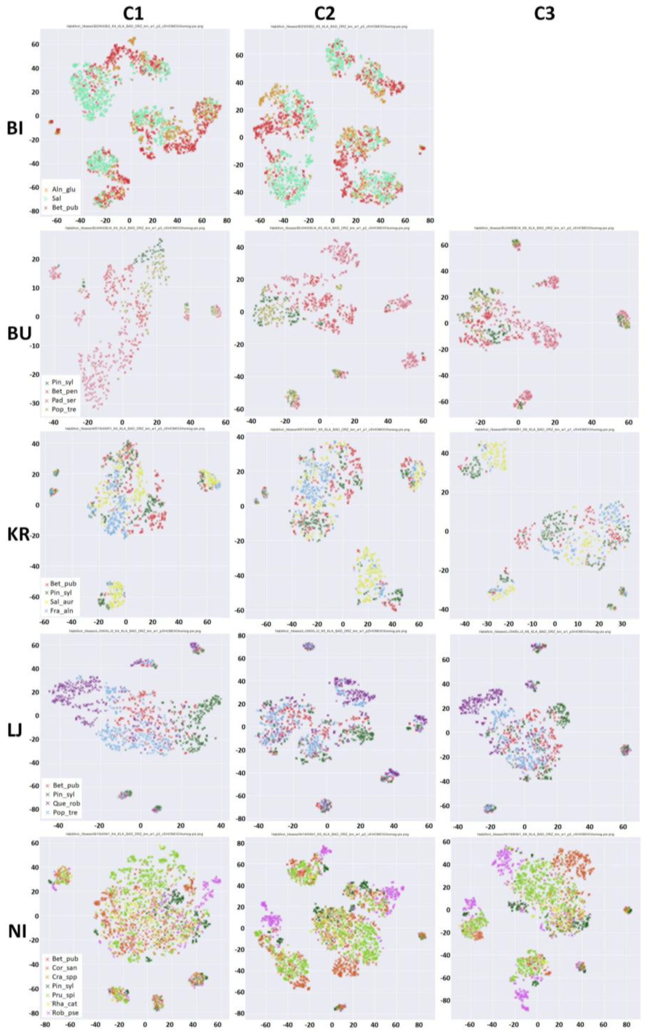
5.1. Results of Implementation of the t-SNE Algorithm

Figure 3 presents the results of the t-SNE algorithm for each research area and data acquisition date analysed. Regardless of the study area, it can be observed that the separability level characterising the pixels forming the reference polygons for the individual species was different for the three data acquisition times analysed. Since the t-SNE analysis was prepared using both hyperspectral (MNF products and vegetation indices) and LiDAR data products, it can be observed that for most of the species, the pixels representing them were divided into a few groups characterised by similar spectral and geometric characteristics.

The results of the t-SNE analysis obtained for the BI research area using spring (C1) and summer (C2) data both show that a proportion of the pixels share similar features. When analysing the separability of individual species, it was noted that better classification results of Alnus glutinosa (shown in orange in Figure 3) are expected to be obtained using the summer (C2) data than when using spring (C1) ones. On the other hand, the classification accuracy of Betula pubescens (shown in red in Figure 3) and Salix spp. (shown in green in Figure 3) is expected to be similar regardless of the data acquisition time.

From the t-SNE results obtained for the BU research area using the spring (C1) data collection, it can be observed that individual species demonstrate a high level of separability. Only Betula pendula (shown in red in Figure 3) is not fully separable, which can lead to a low classification accuracy and mixing with Populus tremula (shown in olive in Figure 3) and Prunus serotina (shown in pink in Figure 3). Additionally, a lower level of separability for Betula pendula, and mixing of pixels representing all species can be observed for t-SNE results prepared using summer (C2) and autumn (C3) data. This may lead to lower classification accuracies compared to those for spring (C1) data.

In case of the KR research area, the results of t-SNE analysis show that the highest separability between species was achieved using the autumn (C3) campaign data. The smallest homogeneity of all the analysed species was found for Betula pendula (shown in red in Figure 3) and Frangula alnus (shown in blue in Figure 3). T-SNE graphs obtained using data acquired in spring (C1) and summer (C2) show that only a proportion of the reference pixels are characterised by a high homogeneity level, and that separability of individual species is lower than for the autumn (C3) data.

The results of a t-SNE analysis for the LJ research area show that the highest separability between species was achieved using the spring (C1) data, and it was expected that the highest classification accuracy would also be obtained for this data. Most of the reference pixels of Quercus robur (shown in violet in Figure 3), Pinus sylvestris (shown in green in Figure 3) and Populus tremula (shown in blue in Figure 3) form clearly distinguishable groups with similar spectral and geometrical properties. The species that stands out is Betula pendula (marked in red in Figure 3), which is characterised by the lowest homogeneity and separability.

The highest homogeneity and separability of the species present in the NI research area was found for Robinia pseudoacacia (shown in magenta in Figure 3), and especially in the graphs prepared using summer (C2) and autumn (C3) data. It can therefore be expected that a high classification accuracy could be obtained using these data for this species. Moreover, relatively high levels of homogeneity and separability were also obtained for Cornus sanguinea (shown in orange in Figure 3), Prunus spinosa (shown in green in Figure 3) and Pinus sylvestris (shown in dark green in Figure 3) using the summer (C2) and autumn (C3) campaign data. On the other hand, the lowest separability was found for Rhamnus cathartica (shown in yellow in Figure 3) and Crataegus sp. (shown in light orange in Figure 3). It can also be observed that the biggest mixing of the reference pixels of different species was found in the graphs prepared using spring (C1) data; only a certain proportion of the reference pixels of Robinia pseudoacacia, Pinus sylvestris, Prunus spinosa and Cornus sanguinea formed groups with similar spectral and geometrical properties.

5.2. Results of Accuracy Assessment

The highest classification accuracy for succession species was obtained for the KR research area, using data acquired in autumn (C3). The variation in the average values of Cohen’s Kappa coefficient for the autumn campaign (C3) was between 0.65 for the LJ research area and 0.85 for the KR research area; for the summer campaign (C2), this was between 0.61 for the LJ research area and 0.81 for the BI research area; and for the spring campaign (C1), this was between 0.52 for the NI research area and 0.79 for the BU research area (Figure 4). Relatively large variations between acquisition dates were observed in the average value of Cohen’s Kappa coefficient for the KR, LJ and NI research areas, while lower differences were found for the two remaining areas, BI and BU. It can also be observed that in most cases, the standard deviation of the Cohen’s Kappa coefficient obtained for different dates and study areas was almost the same, at between 0.03 and 0.04. The only exceptions (slightly higher deviations) were seen in the summer (C2) data for the BU (0.07) and LJ areas (0.06), and in the autumn data (C3) for the LJ area (0.09).

The most accurate classification of the NI research area was obtained using the C3 data, for which the Cohen’s Kappa value was 0.73 (Figure 4). This result was determined by the relatively high classification accuracies of the broadleaved species, and in particular Prunus spinosa (F1 = 0.86), Robinia pseudoacacia (F1 = 0.83) and Cornus sanguinea (F1 = 0.86) (Figure 5). Rhamnus cathartica and Crataegus sp. on the other hand, did not achieve high F1-scores in any of the collections. The highest classification accuracy of Crataegus sp. (0.50) was obtained using data acquired in C1. The results of the accuracy assessment show that the lowest Cohen’s Kappa value (0.52) was obtained for classification of the C1 collection of the NI research area (Figure 4). For this data collection, the highest F1-scores were achieved for Pinus sylvestris (0.75), Prunus spinosa (0.71) and Robinia pseudoacacia (0.65) (Figure 5). All of the other species present in the NI research area were classified with lower accuracies, characterised by F1-scores ranging from 0.37 to 0.59. Pinus sylvestris, the only coniferous species analysed in this area, was classified with approximately equal accuracy using all data collections, and had F1-scores ranging from 0.74 to 0.78 (Figure 5).

Large discrepancies between the classification accuracies obtained for different data acquisition times can also be observed for the KR and LJ research areas. For the former, the Cohen’s Kappa coefficients were 0.69 for summer (C2) and 0.85 for autumn (C3) (Figure 4), while the latter had values of 0.61 for summer (C2) and 0.77 for autumn (C3). The lowest classification accuracy of the KR research area achieved using summer collection data (C2) was mostly determined by the F1-score achieved for Frangula alnus of 0.71 (Figure 5). This species was classified with higher accuracies using late spring (C1) and autumn (C3) data collections, achieving F1-scores of 0.82 and 0.78, respectively. The autumn data collection (C3) was also favourable for classifying Betula pendula and Salix spp., obtaining F1-scores of 0.89 and 0.94, respectively.

The relatively high value of Cohen’s Kappa of 0.77 obtained for the LJ research area using spring data (C1) may have been due to the good discrimination of all species present in the area; all of the obtained F1-scores were approximately 0.1 higher than for the two remaining collections. The lowest value of Cohen’s Kappa (0.61) for the classifications of the LJ area was obtained for the summer data collection (C2), and a slightly higher one of 0.65 was obtained for the autumn data (C3) (Figure 4). It is important to note that Betula pendula was the species with the lowest accuracy; its F1-score ranged between 0.52 and 0.62 for the different data sets, and this strongly influenced the Cohen’s Kappa coefficients (Figure 5).

For the rest of the research areas, i.e., BI and BU, the variation in the values of Cohen’s Kappa obtained using different collections of data were much lower than for the three previously described research areas. It can be observed that the highest classification accuracies were achieved for data acquired in spring (C1) in the case of the BU study area. For the BI area, we could not clearly identify which period was the most suitable for species identification, since only two data collections were carried out and the differences in the values of Cohen’s Kappa were very small.

The lowest variation in the accuracies obtained for two data acquisition times was found for the BI research area (Figure 4). The Cohen’s Kappa values were 0.78 and 0.81 for late spring (C1) and summer (C2), respectively. Of the species present in the BI research area, Alnus glutinosa was classified with the lowest accuracy of 0.76–0.81 (Figure 5).

The accuracy assessment for the summer data collection (C2) of the BU research area indicates that compared to the two other collections, relatively low F1-scores were obtained for Populus tremula (0.69) and Pinus sylvestris (0.63) (Figure 5). The results for the autumn (C3) data also highlight the relatively low accuracy obtained for Betula pendula, for which the F1-score was 0.69. Prunus serotina was classified with relatively high accuracy in all collections of data (Figure 5); the achieved F1-scores were 0.92, 0.91 and 0.89 for spring (C1), summer (C2) and autumn (C3) acquisition times, respectively.

Generalizing the obtained results, it can be stated that in the case of the BU and the LJ research areas (with European dry heaths) the highest accuracy of classification of almost all species was obtained in the C1 campaign (spring), while for the KR and the NI research areas—in the C3 campaign (autumn). The summer period was generally less favourable.

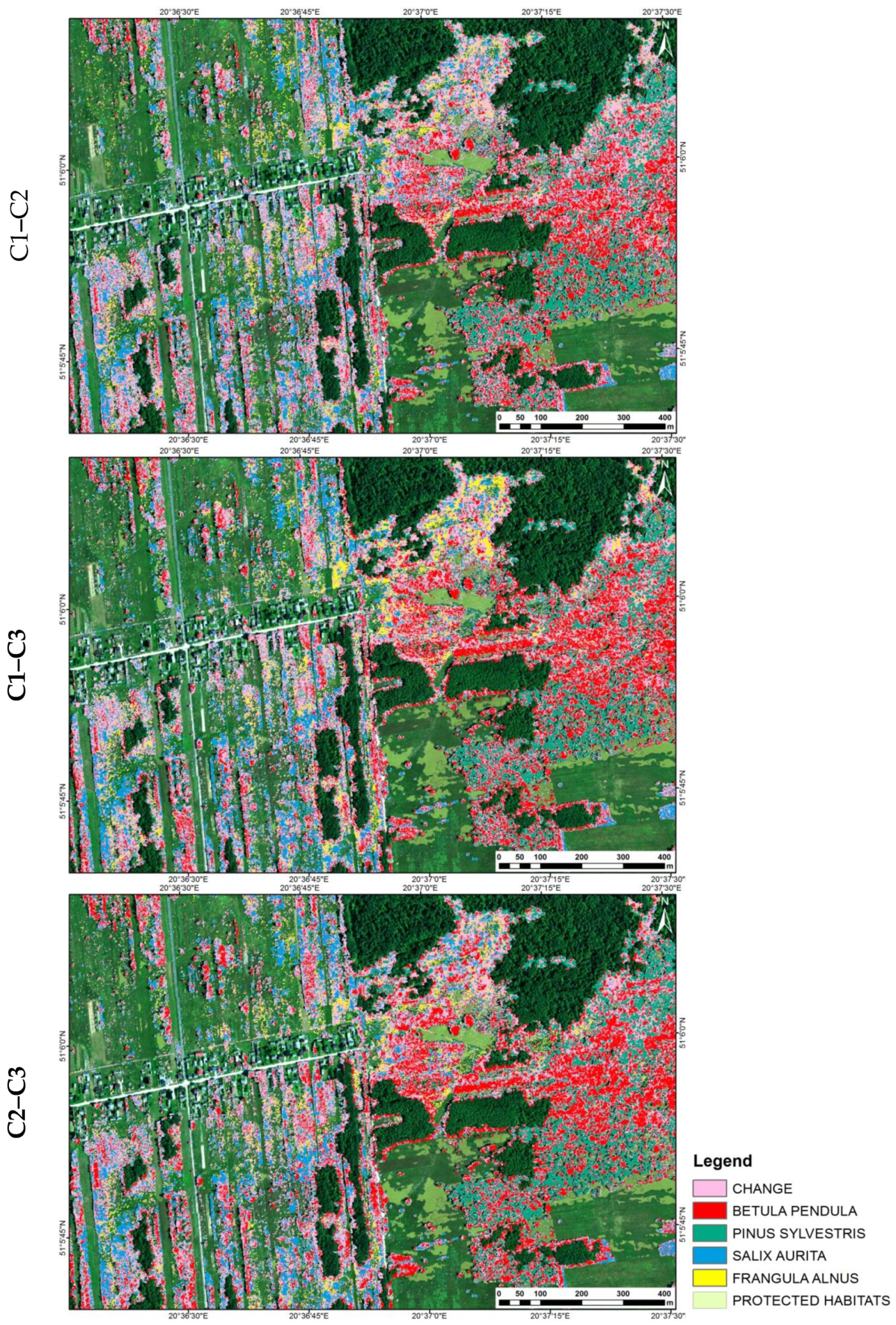
5.3. Comparison of the Extent of Species in Different Seasons

The obtained results also showed the area occupied by trees and shrubs forming the succession process in each study site (

Table 6. Degree of agreement between the spatial extents of species obtained at three data acquisition times for different research areas.

	Study Area
Flight Campaigns	BI	BU	KR	LJ	NI
spring (C1)–summer (C2)	66.8%	59.4%	48.7%	51.9%	46.1%
spring (C1)–autumn (C3)	-	50.7%	49.1%	57.2%	43.8%
summer (C2)–autumn (C3)	-	49.1%	51.9%	53.0%	52.6%
spring (C1)–summer (C2)–autumn (C3)	-	33.7%	31.8%	35.7%	32.2%

). As one aspect of our research, we determined the parts of succession area in which the same species were identified in all three classifications prepared using different data collections. We present this information in Figure 6, Figure 7, Figure 8, Figure 9 and Figure 10, in which the areas of agreement are marked with the colour of the appropriate species and the areas of disagreement between the classification results are marked in pink.

The results of comparative analysis show that only on about 32–36% of area occupied by succession, the same species were identified regardless of the data acquisition time. A comparison of the results of the classifications from two different dates shows that species compliance ranged from approximately 44% to 69%.

6. Discussion

6.1. Influence of Acquisition Date on the Classification Results

6.1.1. BI Research Area

The accuracy of classification of succession species in the case of the BI research area was high for both campaigns analysed (C1 and C2). This was as expected from the t-SNE analysis (Figure 3) and as indicated by the results of the accuracy assessment. The classification accuracies achieved for different species present in the research area were characterised by high stability, with a standard deviation of the F1-score between 0.02 and 0.04. This was probably the result of a relatively large reference data set.

Of the three species classified in the BI area, Alnus glutinosa had the lowest accuracy (F1 = 0.76 in C1 and F1 = 0.81 in C2, Figure 5), and this may be connected with the morphological variability of this species. In spring, the leaves of these specimens are formed relatively late, which may lead to the lower F1-score achieved for this collection (C1), compared to summer acquisition (C2). At the same time, the leaves of Alnus glutinosa remain on the trees for a long time, favouring late summer and autumn acquisition dates, also in adverse atmospheric conditions. The F1-score obtained for Alnus glutinosa for the late spring data collection (C1) may also be lower than the scores achieved for the summer (C2) and autumn (C3) data due to the interplay between the analysed species and the surrounding vegetation types, which are tall herb communities and tall sedges. At the end of June, these vegetation types were fully developed, and thus reached maximum plant coverage.

Similarly high classification accuracies were obtained for the summer data collection (C2), for the remainder of the species present in the BI research area. The crown densities of both Salix spp. and Betula pubescens were approximately the same for all data acquisition times, and there was therefore no factor which could affect their differentiation. On the other hand, the high (0.90–0.91) and stable F1-scores obtained for Salix sp. may be the result of aggregation of three species (Salix cinerea, Salix aurita, Salix rosmarinifolia) into one class.

6.1.2. BU Research Area

The best differentiation of Pinus sylvestris in the BU research area was achieved using data acquired in spring (C1), for which the F1-score reached a value of 0.90. This is also indicated by the results of the t-SNE analysis (Figure 3). The F1-score obtained using summer (C2) data was significantly lower at 0.63, and this can be explained by the fact that Pinus sylvestris is strongly contrasted with the surroundings, where heather often dominates. This contrast is most distinct in spring, while in summer it decreases due to an increase in heather growth. The lower accuracy (and the higher standard deviation of the F1-score) obtained using data acquired in the summer (C2) may also partly be the result of the similarity between the spectral characteristics of small Pinus sylvestris specimens and heather. In the autumn (C3), the contrast between Pinus sylvestris and the surroundings was higher than in the summer, which can be attributed to the blooming of the heather, discolouration and subsequent withering of the grass, and the loss of leaves from deciduous trees and shrubs. As a result, the differentiation of all Pinus sylvestris specimens, including smaller ones, was relatively good in the autumn, as expressed by an F1-score of 0.78.

The autumn discolouration of leaves of Populus tremula did not highly alter the appearance of this species. Nevertheless, this change may have contributed to the slightly higher accuracy obtained using autumn data collection (C3) compared to the other data acquisition times, despite the relatively large loss of leaves and the lower crown densities observed for Populus tremula at that time. Additionally, this species is characterised by high morphological variability, which can also explain the relatively low accuracy of this species compared to the others present in the BU research area; the F1-score achieved for Populus tremula was 0.69 for the C2 data collection, while for Betula pendula this was 0.78 and for Prunus serotina, 0.91 (Figure 5). The accuracy assessment report of the BU autumn (C3) data classification also highlights the relatively low accuracy obtained for Betula pendula, as the F1-score was 0.69. This can be explained by the fact that the analysed species was present in several different types of habitats, from very dry to wetter ones. The humidity strongly affects the phenological changes: in dry habitats, trees lose their leaves and discolour faster than in wet habitats. This kind of situation leads to a higher interspecies differentiation and therefore a more difficult classification problem.

In the BU research area, Prunus serotina was classified with high accuracy in all collections of data (Figure 5), with F1-scores of 0.92, 0.91 and 0.89 for spring (C1), summer (C2) and autumn (C3) acquisition times, respectively. These results can be explained by the various properties that clearly differentiate this species from the others present in the BU research area; in spring, it blossoms, while in summer it has a high crown density, and in autumn the leaves undergo noticeable discolouration. It is also important to stress that the measured specimens of Prunus serotina over the whole season significantly differed from the surrounding land cover.

6.1.3. KR Research Area

In the case of the KR research area, the highest value of Cohen’s Kappa coefficient was obtained in autumn (C3). These data were acquired as the last ones from all analysed areas, i.e., deciduous trees and shrubs were characterised by a significant degree of leaf discoloration, which in turn influenced the better separability of individual species (Figure 3). A relatively low accuracy of classification (as measured by the F1-score) was only found for Frangula alnus, and a slightly higher standard deviation of the F1-score was also noted. However, shrubs of this species have a loose crown, meaning that the spectral response from the pixels representing them is also adulterated by the information coming from the ground or vegetation growing below. This species was classified with the lowest accuracy in the summer campaign (C2), when the accompanying vegetation was fully developed and had a stronger impact on the spectral response recorded in the pixels. In addition, drought may have occurred locally in the summer, causing partial leaf fall and further intensifying the impact of the surroundings on the spectral value of the pixels representing Frangula alnus. A similar situation can be observed in the case of Betula pendula, which is also characterised by a loose crown. The lower homogeneity compared to the other species is visible on the t-SNE graph (Figure 3).

The relatively small difference in the values of the F1-scores obtained for Betula pendula, Pinus sylvestris and Salix aurita can be explained by the fact that remote sensing data of the spring campaign (C1) were acquired relatively late (2 June) and the differences in the vegetation observed between this period and the summer campaign (C2) were not very significant. Vegetation in both campaigns was well developed, and this was caused by weather conditions that were warmer and more humid in the spring and warmer in the summer compared to the average between 1971 and 2000.

6.1.4. LJ Research Area

The best classification results for the succession species present in the LJ research area were obtained for the spring (C1) data. This was as expected on the basis of the t-SNE graph analysis (Figure 3). The lowest Cohen’s Kappa coefficient was obtained for the summer period (C2), which results from the lower homogeneity and separability of the species compared to the other periods, as can be observed in Figure 3. These results may be due to changes in either the stage of development of the surrounding vegetation or the level of discoloration of deciduous leaves.

In all cases, Betula pendula was classified with the lowest accuracy, from 0.52 for the C2 data to 0.61 for the C1 data. The reason for this may be the specificity of this species, which is characterised by a relatively low crown density, meaning that the spectral response from the pixels representing this species is also affected by the surroundings and the vegetation growing below. In summer, the influence of the accompanying vegetation is likely to be even greater, resulting in a lower homogeneity of the Betula pendula reference polygons (Figure 3). This is also visible in the stability of the obtained classification results, as the standard deviation of the F1-score was 0.10. The highest stability, regardless of data acquisition time, was found for Quercus robur, which can be attributed to the specificity of this species; the dense crown gives rise to more spectrally pure reference polygons. The exceptions in this case are only the very young specimens.

6.1.5. NI Research Area

The NI research area is strongly diversified in terms of the tree and shrub species occurring there, which are mainly deciduous species. The high accuracies and hence the precise delimitation of species for the NI area using the autumn campaign (C3) data are likely to be the result of leaf discolouration, which affects their separability. This is also confirmed by the results of the t-SNE analysis. The highest F1 values were obtained for those species that were characterised by good separability. It should however be noted that for most of the species present in the analysed area, the F1-score was rather variable, and the standard deviation obtained for Pinus sylvestris, Robinia pseudoacacia and Crataegus sp. was 0.06.

The extremely low classification accuracy obtained for the NI area using spring (C1) data can be explained by the fact that a wide variety of broadleaved species are present in the area, and in spring (C1) their crown foliage density was not high, especially since the remote sensing data for NI were acquired much earlier than for the other areas. As already mentioned, this phenomenon may have influenced the accuracy of classification of the analysed trees and shrubs. The high classification accuracy of Crataegus sp. (0.50) obtained using data acquired in spring (C1) was probably connected with blossoming.

The low accuracy of classification of Rhamnus cathartica and Crataegus sp. may be related to the similarity between the spectral characteristics of these species and others growing in dry grasslands. Additionally, both species were characterised by relatively small leaves and loose crown leafage, causing the spectral signal to be mixed with the signal from the background. It is also likely that the specimens of the two species were attacked by fungi, and were therefore losing their leaves relatively quickly, with almost no leaves present in autumn.

6.2. Comparative Analysis of Species’ Extent in Different Seasons

Table 6 shows that in about 32–36% of the area occupied by trees and shrubs, the same species were identified regardless of the data acquisition time. The highest degree of agreement between the three classification results was found for the LJ research area. For this study area, a relatively high degree of pairwise agreement was also observed of 51.9%, 53.0% and 57.2% for spring (C1) and summer (C2), summer (C2) and autumn (C3), and spring (C1) and autumn (C3), respectively. The lowest degree of agreement between the different classification results was observed for the NI research area (Table 6), and this can be attributed to the huge variety of tree and shrub species present in the area. In addition to the six succession promoter species analysed here, there were more than 20 other species of trees that could have induced variability in the maps created using data acquired on different dates.

BI was the only research area for which only two rather than three collections of remote sensing data were available. The two classification results obtained were characterised by a high degree of agreement (66.8%). This can be explained by the relatively small number of species present in the area, and the similarity of the appearance of the research objects on two acquisition dates (fully developed tree and shrub crowns). The disagreement between the classification results may have been influenced by the phenological changes in the surrounding vegetation types, i.e., reedbeds, sedge and tall herb communities.

All of the research areas analysed here differed in terms of their characteristics as well as in the composition of tree and shrub species. A detailed investigation of the agreement between the classification results obtained using different data collections and for various Natura 2000 habitats indicated that Pinus sylvestris was the species with the most stable spatial extent. These findings can be attributed to the fact that Pinus sylvestris is a coniferous species, and changes little throughout the growing season. The spatial extents of the broadleaved species were substantially more dependent on the data collection used to provide the classification product. In the case of BI (a wetland research area), the highest degree of agreement between the different classification results was found for Alnus glutinosa and Betula pubescens, while the lowest was seen for Salix spp. The lower performance for Salix spp. can be explained by the characteristics of its occurrence in the BI study area, such as the influence of the co-occurring vegetation types and their structure: small willow shrubs were growing between tall sedge clumps, or were being overgrown by tall herb or reed communities. The results obtained for the LJ research area, which included heaths, indicated that the highest stability of the spatial extent was found for Pinus sylvestris and Betula pendula, and the lowest stability for Quercus robur. The specimens of Quercus robur were small, and their characteristics in the remote sensing data were therefore highly influenced by the surrounding vegetation and its phenological changes. Similar observations could be made regarding the agreement between classifications prepared using different collections of data for Pinus sylvestris and Betula pendula in the KR research area. In this study site, the spatial extent of Frangula alnus and Salix spp. showed the strongest dependence on the data collection used.

An analysis of Figure 6, Figure 7, Figure 8, Figure 9 and Figure 10 and Figure A1, Figure A2, Figure A3 and Figure A4 in Appendix B allow us to conclude that the discrepancies between classification results were primarily related to smaller trees and shrubs or groups (in all study areas), and other species characterised by low crown density such as Frangula alnus, Betula pubescens, Betula pendula and Populus tremula. Apart from these specimens, discrepancies were also identified at the borders of tree and shrub clumps (groups), thus demonstrating the influence of the surroundings. This is a well-known problem of so-called mixed pixels, which in this case involves a mixture of the analysed species and the background vegetation types, e.g., tall herb communities, sedge communities, reed beds or heath. The discrepancies in the classification results were also related to the less frequently occurring species that were outside of the scope of the research, for which reference data were not collected, and which were often present outside the borders of the Natura 2000 habitats. This type of discrepancy was especially noticeable in research areas characterised by a high variety of broadleaved species e.g., KR or NI. In the case of the KR research area, it was also seen, that the classification results for Frangula alnus in the C1 (spring) and C3 (autumn) campaigns showed big agreement (Figure A3 in Appendix B), while comparing the results for the campaign pairs C1 (spring)–C2 (summer), and C2 (summer)–C3 (autumn) this agreement was much weaker. This is the result of lower classification accuracy for the summer campaign (C2) (Figure 5). And this was due to the significant impact of the surrounding—well-developed herbaceous plants, in this period—and its spectral response. In spring they were in the early stages of growing, and in autumn Frangula alnus, due to discoloration, stood out more strongly against the background.

6.3. Comparison of the Obtained Results with Previous Research Studies

The classification results for succession species obtained here were compared to those of previous research studies that were selected from the literature as representative. The most important features of these studies are presented in

Table A1. Comparison of the classification accuracy of selected species of European trees succession promoters in Poland) obtained by various research teams. HS—airborne hyperspectral imagery; LiDAR—airborne LiDAR data; PA—producer’s accuracy; UA—user’s accuracy; OA—overall accuracy; K—Cohen’s kappa coefficient.

Authors of the Study	Acquisition Data	Type of Data	Methods	No. of Classes/OA/K	Species of Interest	Accuracy
Dalponte et al., 2008 [56]	28 June 2006	HS, 1 m; LiDAR, 5.6 pt/m2	Support vector machines	23/-/0.88	Alnus glutinosa Quercus robur Robinia pseudoacacia	PA: 0.910 PA: 0.882 PA: 0.882
Dalponte et al., 2012 [36]	16 July 2008	HS, 1 m; LiDAR, 8.6 pt/m2	Support vector machines	8/-/0.772	Pinus sylvestris	PA: 0.843, UA: 0.820
Immitzer et al., 2012 [37]	10 July 2010	WorldView-2, 2 m	Random forest	10/0.728/0.678	Alnus glutinosa Betula pendula Quercus robur Pinus sylvestris	PA: 0.823, UA: 0.775 PA: 0.872, UA: 0.872 PA: 0.921, UA: 0.854 PA: 0.739, UA: 0.829
Priedītis et al., 2015 [91]	27 October 2014	HS, 0.5 m	Linear discriminant analysis	5/-/-	Alnus glutinosa Betula pendula Pinus sylvestris Populus tremula	PA: 0.563 PA: 0.770 PA: 0.948 PA: 0.714
Raczko & Zagajewski 2017 [88]	10 September 2012	HS, 2.5 m	Random forest	5/0.62/0.52	Betula pendula	PA: 0.50, UA: 0.55
Raczko & Zagajewski 2017 [88]	10 September 2012	HS, 2.5 m	Support vector machines	5/0.68/0.61	Betula pendula	PA: 0.59, UA: 0.57
Raczko & Zagajewski 2017 [88]	10 September 2012	HS, 2.5 m	Artificial neural networks	5/0.77/0.72	Betula pendula	PA: 0.68, UA: 0.69
Richter et al., 2016 [64]	2 August 2013	HS, 2 m	Partial least square discriminant analysis	10/0.705/-	Alnus glutinosa Quercus robur	PA: 0.78, UA: 0.69 PA: 0.72, UA: 0.58
Richter et al., 2016 [64]	25 September 2011	HS, 2 m	Partial least square discriminant analysis	10/0.746/-	Alnus glutinosa Quercus robur	PA: 0.56, UA: 0.55 PA: 0.44, UA: 0.52
Richter et al., 2016 [64]	2 August 2013 and 25 September 2011	HS, 2 m	Partial least square discriminant analysis	10/0.784/-	Alnus glutinosa Quercus robur	PA: 0.89, UA: 0.86 PA: 0.59, UA: 0.64
Trier et al., 2018 [46]	2 May - 20 June 2015	HS, 1 m; LiDAR, 5 pt/m2	Deep neural network	3/0.78/-	Pine Birch	PA: 1.00, UA: 0.88 PA: 0.70, UA: 0.61
Tuominen et al., 2018 [91]	21 August 2015	HS, 20 cm; DSM	K-nearest neighbour method + genetic algorithm	14/0.823/0.808	Betula spp. Pinus spp. Populus spp. Quercus spp.	PA: 0.40, UA: 1.00 PA: 0.97, UA: 0.91 PA: 0.63, UA: 0.86 PA: 0.92, UA: 0.84
Wietecha et al., 2019 [89]	19 August 2015	HS, 2.5 m, 5 m; LiDAR, 10 pt/m2	Support vector machines	5/0.922/0.810	Alnus glutinosa Betula pendula Quercus robur	PA: 0.813, OA: 0.591 PA: 0.656, OA: 0.778 PA: 0.964, OA: 0.962

(in Appendix A). It should be noted that although numerous research studies have been published on the topic of species classification, they mostly concern forest environments rather than agricultural areas described in this study, and cover all types of climatic zones, including some that are very different from those in Poland, e.g., the tropics. In this comparative analysis, we therefore primarily examined forest research studies carried out in Europe. For this reason, it should be borne in mind that the research objects and related challenges may be rather different from those of the present study. Finally, it should also be noted that a variety of statistical measures were used in the analysed articles, making a comparison more difficult. For this reason, the F1-score was also calculated by the present authors for those studies in which the necessary statistical measures were available.

Based on the information presented in Table A1 (in Appendix A), it can be observed that the acquisition dates of the data used by these different authors cover almost a whole growing season, i.e., from May to October. This indicates that the best date for differentiating tree and shrub species has not yet been determined, and proves that the present research is valuable. Moreover, it should be noted that in most studies, airborne rather than VHR satellite data were used; this can be attributed to the low availability of satellite imagery characterised by high spatial and spectral resolutions that is required for this kind of research. In some of these studies, only spectral (multispectral or hyperspectral) data were used, while in the remainder LiDAR or other geometry-related information was included. It can also be seen from Table A1 (in Appendix A) that many different classifiers were used for species differentiation, such as support vector machines, random forest and neural networks.

The classification accuracies of succession species obtained by different authors varied, and were mostly average or high. Pinus sylvestris was classified with high accuracy in all studies, irrespective of the data acquisition time, similarly to the present study. The possibility of a highly accurate classification of Pinus sylvestris using spring data was also confirmed in all research areas in the current work. However, the accuracies obtained for Betula pendula were diverse, and are likely to be dependent on the character of the research area, the type and density of the forest stands, the remote sensing data acquisition time, and the classification strategies and algorithms used. The results obtained in the present research using spring data are similar (LJ area) or better (BU area) than those achieved by Trier et al. [46]. The F1-scores obtained in this research using summer data are similar to those of Immitzer et. al. [37], and are poorer by 0.11–0.15 than those of Trier et al. [46]. This may be because the research of Trier et al. [46] concerned dense forest stands, while the present study involved smaller groups of threes or single specimens. Based on Table A1 (in Appendix A), it can be observed that Betula pendula was classified less accurately using early September data than using the other data sets, both in this research and in the study of Raczko and Zagajewski [88]. Slightly better results for classification of this species were obtained by Wietecha et al. [89] using data acquired in August. Alnus glutinosa was characterised by a range of different accuracies that were dependent on the acquisition time of the data. It can be seen from Table A1 (in Appendix A) that data acquired in autumn did not enable high classification accuracies to be obtained for this species [64, 90]. This could not be confirmed in the current study due to the unavailability of suitable autumn data; however, the results obtained for other acquisition times conform to those achieved in the present research. The classification results obtained using summer campaign data were slightly better than those achieved by Richter et al. [64] (F1-score 0.03 higher) and Wietecha et al. [89] (F1-score 0.14 higher). The classification accuracies obtained in this research for Quercus robur are also comparable to those achieved by the other authors [37,56,91]. Only Wietecha et al. [89] achieved higher values, using data acquired at a similar time (F1-score 0.1 higher), although it should be noted that their research concerned forest stands. The results of Richter et al. [64] are much lower (for both summer and autumn data collection); this is probably due to the spatial resolution of the data used (2 m rather than 1 m) or, in the case of the autumn data, by a spectral similarity to other species. No prior work was found in which this species was classified using spring data, which in the present research was shown to be the most favourable. This may be due to significant differences in spectral properties between this species and the others present in the LJ research area. The classification accuracies achieved for Populus tremula using summer and autumn remote sensing data are similar in the present research and in studies by the other authors [90,91]; however, based on the results of this research, it seems that spring is more favourable for classifying this species (F1-score approximately 0.1 higher than for other dates). The current study is the first to show this possibility. Comparable classification accuracies to those of the summer and autumn data collections reported in this study were also obtained for Robinia pseudoacacia by Dalponte et al. [48] using remote sensing data collected in late June. In the present research, the worst results were obtained using spring data, since the trees did not have fully developed leafage, and this in turn determined the lower homogeneity of their reference polygons.

In summary, we can conclude that the results obtained in the present research are similar or slightly better than those achieved by other authors, even though this study involved smaller research objects that are more difficult to classify.

7. Conclusions

In order to preserve the valuable resources (i.e., habitats and species) of the Natura 2000 areas, monitoring of these habitats and their threats needs to be conducted. An innovative approach to this monitoring is offered by the use of remote sensing data and state-of-the-art algorithmic techniques providing beneficiaries with a comprehensive approach covering all important aspects of the research phenomenon, a large scale of the study, as well as repeatable results based on clearly defined, precise measures and indices.

In this study, the influence of the date of remote sensing data acquisition on the possibility of differentiating succession species was assessed. The aim of the research was to identify whether it is viable to determine a single optimal time period for this goal, rather than carrying out several separate flights, as this would make the methodology more efficient and financially viable. It is worth mentioning that this kind of broad scale research, conducted over several research areas located in different parts of Poland, on three acquisition dates, has not previously been carried out. According to the literature review, it appears that so far no such studies have been carried out at the early stages of succession anywhere in the world, or for such diverse research areas, including different types of habitats.

Based on the results of the research conducted here, it can be concluded that the accuracy of classification of tree and shrub succession species is influenced by multiple factors. These include not only the remote sensing data acquisition time, but also the character of the analysed area, i.e., the diversity and types of deciduous tree and shrub species, the background vegetation types, and the abiotic (water and soil) conditions.

As shown in the study presented here, succession tree and shrub species can be classified with relatively high accuracy regardless of the time of acquisition of remote sensing data. It can however be observed that data collected in spring and autumn are slightly more favourable than data collected in summer for differentiation of most species, provided that the data are not acquired too early (before the full development of leafage) or too late (after the loss of leaves). This conclusion is valid for sites with similar climatic and habitat conditions to those analysed in our study. In the case of places located at the same latitude, but in different climatic zones with a different composition of species, it may be different. Nevertheless, in order to determine the optimal data acquisition time for given site, various factors should be taken into account. Firstly, the phenological cycle of the species present in the research area should be carefully studied, for example the dates of growth, flowering, leaf discoloration and loss characterising deciduous species, as well as the surrounding vegetation. The abiotic conditions influencing vegetation growth should also be taken into account.

The results of classifying succession species achieved in this study are similar or in some cases better than those reported by other authors, whose studies were mostly done in forest environments. However, the research conducted here also enabled us to highlight issues that should be investigated further in the future. Firstly, the correctness of the reference polygons, and therefore their homogeneity, as a crucial element of the classification process, should carefully be studied. Secondly, it should be determined whether the LiDAR data set, which is complementary to hyperspectral one, is necessary for species differentiation and whether the difference in accuracy achieved justifies the costs of acquiring the additional dataset. Finally, an analysis of the differences between the spatial extents of species obtained using data from different acquisition dates should be extended to single species, and the impact of the habitat type should be analysed.

References

1. EEA. EU Biodiversity Strategy to 2020. Available online: https://eur-lex.europa.eu/legal-content/EN/TXT/PDF/?uri=CELEX:52011DC0244&from=EN (accessed on 10 June 2019).
2. Waldron, A.; Miller, D.C.; Redding, D.; Mooers, A.; Kuhn, T.S.; Nibbelink, N.; Roberts, J.T.; Tobias, J.A.; Gittleman, J.L. Reductions in global biodiversity loss predicted from conservation spending. Nature 2017, 551, 364–367. [Google Scholar] [CrossRef] [PubMed]
3. Cardinale, B.J.; Duffy, J.E.; Gonzalez, A.; Hooper, D.U.; Perrings, C.; Venail, P.; Narwani, A.; Mace, G.M.; Tilman, D.; Wardle, D.A.; et al. Biodiversity loss and its impact on humanity. Nature 2012, 486, 59–67. [Google Scholar] [CrossRef] [PubMed]
4. EEA. EU Biodiversity Action Plan. Available online: http://ec.europa.eu/environment/nature/ biodiversity/comm2006/index_en.htm (accessed on 10 June 2019).
5. Chan, J.C.W.; Spanhove, T.; Ma, J.; Borre, J.V.; Paelinckx, D.; Canters, F. Natura 2000 habitat identification and conservation status assessment with superresolution enhanced hyperspectral (CHRIS/Proba) Imagery. In Proceedings of the GEOBIA 2010 Geographic Object-Based Image Analysis, Ghent, Belgium, 29 June–2 July 2010. [Google Scholar]
6. Lucas, R.; Medcalf, K.; Brown, A.; Bunting, P.; Breyer, J.; Clewley, D.; Keyworth, S.; Blackmore, P. Updating the phase 1 habitat map of Wales UK, using satellite sensor data. ISPRS J. Photogrammetry Remote Sens. 2011, 66, 81–102. [Google Scholar] [CrossRef]
7. Schuster, C.; Schmidt, T.; Conrad, C.; Kleinschmit, B.; Förster, M. Grassland habitat mapping by intra-annual time series analysis–comparison of RapidEye and TerraSAR-X satellite data. Int. J. Appl. Earth Obs. Geoinf. 2015, 34, 25–34. [Google Scholar] [CrossRef]
8. Haest, B.; Vanden Borre, J.; Spanhove, T.; Thoonen, G.; Delalieux, S.; Kooistra, L.; Mücher, C.A.; Paelinckx, D.; Scheunders, P.; Kempeneers, P. Habitat mapping and quality assessment of NATURA 2000 heathland using airborne imaging spectroscopy. Remote Sens. 2017, 9, 266. [Google Scholar] [CrossRef]
9. Mahdianpari, M.; Salehi, B.; Mohammadimanesh, F.; Homayouni, S.; Gill, E. The first wetland inventory map of Newfoundland at a spatial resolution of 10 m using Sentinel-1 and Sentinel-2 data on the Google Earth engine cloud computing platform. Remote Sens. 2019, 11, 43. [Google Scholar] [CrossRef]
10. Zlinszky, A.; Deák, B.; Kania, A.; Schroiff, A.; Pfeifer, N. Mapping Natura 2000 habitat conservation status in a Pannonic salt steppe with airborne laser scanning. Remote Sens. 2015, 7, 2991–3019. [Google Scholar] [CrossRef]
11. Schmidt, J.; Fassnacht, F.E.; Forster, F.; Schmidtlein, S. Synergetic use of Sentinel-1 and Sentinel-2 for assessments of heathland conservation status. Remote Sens. Ecol. Conserv. 2017, 4, 225–239. [Google Scholar] [CrossRef] [Green Version]
12. Huang, C.Y.; Asner, G.P. Applications of remote sensing to alien invasive plant studies. Sensors 2009, 9, 4869–4889. [Google Scholar] [CrossRef] [PubMed]
13. Dorigo, W.; Lucieer, A.; Podobnikar, T.; Carni, A. Mapping invasive Fallopia japonica by combined spectral, spatial, and temporal analysis of digital orthophotos. Int. J. Appl. Earth Obs. Geoinf. 2012, 19, 185–195. [Google Scholar] [CrossRef]
14. Bradley, B.A. Remote detection of invasive plants: A review of spectral, textural and phenological approaches. Biol. Invasions 2014, 16, 1411–1425. [Google Scholar] [CrossRef]
15. Marcinkowska-Ochtyra, A.; Jarocińska, A.; Bzdęga, K.; Tokarska-Guzik, B. Classification of expansive grassland species in different growth stages based on hyperspectral and LiDAR data. Remote Sens. 2018, 10, 2019. [Google Scholar] [CrossRef]
16. Batistella, M.; Lu, D. Integrating field data and remote sensing to identify secondary succession stages in the Amazon. In Proceedings of the 29th International Symposium on Remote Sensing of Environment, Buenos Aires, Argentina, 8–12 April 2002. [Google Scholar]
17. Szostak, M.; Wężyk, P.; Hawryło, P.; Puchała, M. Monitoring the secondary forest succession and land cover/use changes of the Błędów Desert (Poland) using geospatial analyses. Quaest. Geogr. 2016, 35, 5–13. [Google Scholar] [CrossRef]
18. Osińska-Skotak, K.; Jełowicki, Ł.; Bakuła, K.; Michalska-Hejduk, D.; Wylazłowska, J.; Kopeć, D. Analysis of using dense image matching techniques to study the process of secondary succession in non-forest Natura 2000 habitats. Remote Sens. 2019, 11, 893. [Google Scholar] [CrossRef]
19. Dabrowska-Zielinska, K.; Musial, J.; Malinska, A.; Budzynska, M.; Gurdak, R.; Kiryla, W.; Bartold, M.; Grzybowski, P. Soil moisture in the Biebrza Wetlands retrieved from Sentinel-1 imagery. Remote Sens. 2018, 10, 1979. [Google Scholar] [CrossRef]
20. Perennou, C.; Guelmami, A.; Paganini, M.; Philipson, P.; Poulin, B.; Strauch, A.; Tottrup, C.; Truckenbrodt, J.; Geijzendorffer, I.R. Mapping Mediterranean wetlands with remote sensing: A good-looking map is not always a good map. Adv. Ecol. Res. 2018, 58, 243–277. [Google Scholar]
21. Ciężkowski, W.; Jóźwiak, J.; Szporak-Wasilewska, S.; Dabrowski, P.; Góraj, M.; Kleniewska, M.; Chormański, J. Water stress index for bogs and mires based on UAV land surface measurements and its dependency on airborne hyperspectral data. In Proceedings of the 2018 IEEE International Geoscience and Remote Sensing Symposium, Valencia, Spain, 22–27 July 2018. [Google Scholar]
22. Ostermann, O.P. The need for management of nature conservation sites designated under Natura 2000. J. Appl. Ecol. 1998, 35, 968–973. [Google Scholar] [CrossRef]
23. Halada, L.; Evans, D.; Romão, C.; Petersen, J.E. Which habitats of European importance depend on agricultural practices? Biodivers. Conserv. 2011, 20, 2365–2378. [Google Scholar] [CrossRef]
24. Prévosto, B.; Kuiters, L.; Bernhardt-Römermann, M.; Dölle, M.; Schmidt, W.; Hoffmann, M.; Van Uytvanck, J.; Bohner, A.; Kreiner, D.; Stadler, J.; et al. Impacts of Land Abandonment on Vegetation: Successional Pathways in European Habitats. Folia Geobot. 2011, 46, 303–325. [Google Scholar] [CrossRef] [Green Version]
25. Barabasz, B. Wpływ modyfikacji tradycyjnych metod gospodarowania na przemiany roślinności łąk z klasy Molinio-Arrhenatheretea. (The effect of traditional management methods modifications on changes in meadows of Molinio-Arrhenatheretea class). Wiadomości Bot. 1994, 38, 85–94. [Google Scholar]
26. Falińska, K. Plant population processes in the course of forest succession in abandoned meadows. I. Variability and diversity of floristic composition, and biological mechanisms of species turnover. Acta Soc. Bot. Pol. 1989, 58, 439–465. [Google Scholar] [CrossRef]
27. Falińska, K. Plant population processes in the course of forest succession in abandoned meadows. II. Demography and succession promotors. Acta Soc. Bot. Pol. 1989, 58, 467–491. [Google Scholar] [CrossRef]
28. Mróz, W. Monitoring Siedlisk Przyrodniczych. Przewodnik Metodyczny [Natura 2000 Habitat Monitoring]; Part I; Biblioteka Monitoringu Środowiska: Warszawa, Poland, 2010. [Google Scholar]
29. Mróz, W. Monitoring Siedlisk Przyrodniczych. Przewodnik Metodyczny [Natura 2000 Habitat Monitoring]; Part II; Biblioteka Monitoringu Środowiska: Warszawa, Poland, 2012. [Google Scholar]
30. Mróz, W. Monitoring Siedlisk Przyrodniczych. Przewodnik Metodyczny [Natura 2000 Habitat Monitoring]; Part III; Biblioteka Monitoringu Środowiska: Warszawa, Poland, 2013. [Google Scholar]
31. Rohde, W.G.; Olson, C.E., Jr. Multispectral sensing of forest tree species. Photogramm. Eng. Remote. Sens. 1972, 38, 1209–1215. [Google Scholar]
32. Rignot, E.J.M.; Williams, C.L.; Way, J.; Viereck, L.A. Mapping of forest types in Alaskan boreal forests using SAR imagery. IEEE Trans. Geosci. Remote Sens. 1994, 32, 1051–1059. [Google Scholar] [CrossRef] [Green Version]
33. Saatchi, S.; Rignot, E. Classification of boreal forest cover types using SAR images. Remote Sens. Environ. 1997, 60, 270–281. [Google Scholar] [CrossRef] [Green Version]
34. Boschetti, M.; Boschetti, L.; Oliveri, S.; Casati, L.; Canova, I. Tree species mapping with airborne hyper-spectral MIVIS data: The Ticino Park study case. Int. J. Remote Sens. 2007, 28, 1251–1261. [Google Scholar] [CrossRef]
35. Suratno, A.; Seielstad, C.; Queen, L. Tree species identification in mixed coniferous forest using airborne laser scanning. ISPRS J. Photogramm. Remote Sens. 2009, 64, 683–693. [Google Scholar] [CrossRef]
36. Dalponte, M.; Bruzzone, L.; Gianelle, D. Tree species classification in the Southern Alps based on the fusion of very high geometrical resolution multispectral/hyperspectral images and LiDAR data. Remote Sens. Environ. 2012, 123, 258–270. [Google Scholar] [CrossRef]
37. Immitzer, M.; Atzberger, C.; Koukal, T. Tree species classification with random forest using very high spatial resolution 8-band WorldView-2 satellite data. Remote Sens. 2012, 4, 2661–2693. [Google Scholar] [CrossRef]
38. Ørka, H.O.; Dalponte, M.; Gobakken, T.; Næsset, E.; Ene, L.T. Characterizing forest species composition using multiple remote sensing data sources and inventory approaches. Scand. J. For. Res. 2013, 28, 677–688. [Google Scholar] [CrossRef]
39. Korpela, I.; Mehtätalo, L.; Seppänen, A.; Kangas, A. Tree species identification in aerial image data using directional reflectance signatures. Silva Fenn. 2014, 48, 1087. [Google Scholar] [CrossRef]
40. Somers, B.; Asner, G.P. Tree species mapping in tropical forests using multi-temporal imaging spectroscopy: Wavelength adaptive spectral mixture analysis. Int. J. Appl. Earth Obs. Geoinf. 2014, 31, 57–66. [Google Scholar] [CrossRef]
41. Ballanti, L.; Blesius, L.; Hines, E.; Kruse, B. Tree species classification using hyperspectral imagery: A comparison of two classifiers. Remote Sens. 2016, 8, 445. [Google Scholar] [CrossRef]
42. Hauglin, M.; Ørka, H.O. Discriminating between native Norway spruce and invasive Sitka spruce—A comparison of multitemporal Landsat 8 imagery, aerial images and airborne laser scanner data. Remote Sens. 2016, 8, 363. [Google Scholar] [CrossRef]
43. Ørka, H.O.; Hauglin, M. Use of remote sensing for mapping of non-native conifer species. INA Fagrapp. 2016, 33, 76. [Google Scholar]
44. Piiroinen, R.; Heiskanen, J.; Maeda, E.; Viinikka, A.; Pellikka, P. Classification of tree species in a diverse African agroforestry landscape using imaging spectroscopy and laser scanning. Remote Sens. 2017, 9, 875. [Google Scholar] [CrossRef]
45. Shen, X.; Cao, L. Tree-species classification in subtropical forests using airborne hyperspectral and LiDAR data. Remote Sens. 2017, 9, 1180. [Google Scholar] [CrossRef]
46. Trier, Ø.D.; Salberg, A.B.; Kermit, M.; Rudjord, Ø.; Gobakken, T.; Næsset, E.; Aarsten, D. Tree species classification in Norway from airborne hyperspectral and airborne laser scanning data. Eur. J. Remote Sens. 2018, 51, 336–351. [Google Scholar] [CrossRef]
47. Grabska, E.; Hostert, P.; Pflugmacher, D.; Ostapowicz, K. Forest stand species mapping using the Sentinel-2 time series. Remote Sens. 2019, 11, 1197. [Google Scholar] [CrossRef]
48. Voss, M.; Sugumaran, R. Seasonal effect on tree species classification in an urban environment using hyperspectral data, LiDAR, and an object-oriented approach. Sensors 2008, 8, 3020–3036. [Google Scholar] [CrossRef] [PubMed]
49. Jensen, R.R.; Hardin, P.J.; Hardin, A.J. Classification of urban tree species using hyperspectral imagery. Geocarto Int. 2012, 27, 443–458. [Google Scholar] [CrossRef]
50. Zhang, K.; Hu, B. Individual urban tree species classification using very high spatial resolution airborne multi-spectral imagery using longitudinal profiles. Remote Sens. 2012, 4, 1741–1757. [Google Scholar] [CrossRef]
51. Zhang, C.; Qiu, F. Mapping individual tree species in an urban forest using airborne LiDAR data and hyperspectral imagery. Photogramm. Eng. Remote Sens. 2012, 78, 1079–1087. [Google Scholar] [CrossRef]
52. Alonzo, M.; Bookhagen, B.; Roberts, D.A. Urban tree species mapping using hyperspectral and LiDAR data fusion. Remote Sens. Environ. 2014, 148, 70–83. [Google Scholar] [CrossRef]
53. Chance, C.M.; Coops, N.C.; Crosby, K.; Aven, N. Spectral wavelength selection and detection of two invasive plant species in an urban area. Can. J. Remote. Sens. 2016, 41, 1–14. [Google Scholar] [CrossRef]
54. Brabant, C.; Alvarez-Vanhard, E.; Laribi, A.; Morin, G.; Thanh Nguyen, K.; Thomas, A.; Houet, T. Comparison of hyperspectral techniques for urban tree diversity classification. Remote Sens. 2019, 11, 1269. [Google Scholar] [CrossRef]
55. Fassnacht, F.E.; Latifi, H.; Stereńczak, K.; Modzelewska, A.; Lefsky, M.; Waser, L.T.; Straub, C.; Ghosh, A. Review of studies on tree species classification from remotely sensed data. Rem. Sens. Environ. 2016, 186, 64–87. [Google Scholar] [CrossRef]
56. Dalponte, M.; Bruzzone, L.; Gianelle, D. Fusion of hyperspectral and LIDAR remote sensing data for classification of complex forest areas. IEEE Trans. Geosci. Remote Sens. 2008, 46, 1416–1427. [Google Scholar] [CrossRef]
57. Coops, N.C.; Hilker, T.; Wulder, M.A.; St-Onge, B.; Newnham, G.; Siggins, A.; Trofymow, J.A. Estimating canopy structure of Douglas-fir forest stands from discrete-return LiDAR. Trees-Struct. Funct. 2007, 21, 295–310. [Google Scholar] [CrossRef]
58. Ørka, H.O.; Næsset, E.; Bollandsås, M. Classifying species of individual trees by intensity and structure features derived from airborne laser scanner data. Remote Sens. Environ. 2009, 113, 1163–1174. [Google Scholar] [CrossRef]
59. Key, T.; Warner, T.A.; McGraw, J.B.; Fajvan, M.A. A comparison of multispectral and multitemporal information in high spatial resolution imagery for classification of individual tree species in a temperate hardwood forest. Remote Sens. Environ. 2001, 75, 100–112. [Google Scholar] [CrossRef]
60. Matthew, E.F.; DeFries, R.S.; Sesnie, S.E.; Arroyo-Mora, J.P.; Soto, C.; Singh, A.; Townsend, P.A.; Chazdon, R.L. Mapping species composition of forests and tree plantations in Northeastern Costa Rica with an integration of hyperspectral and multitemporal Landsat imagery. Remote Sens. 2015, 7, 5660–5696. [Google Scholar]
61. Hościło, A.; Lewandowska, A. Mapping forest type and tree species on a regional scale using multi-temporal Sentinel-2 data. Remote Sens. 2019, 11, 929. [Google Scholar] [CrossRef]
62. Mickelson, J.G.; Civco, D.L.; Silander, J.A. Delineating forest canopy species in the northeastern United States using multi-temporal TM imagery. Photogramm. Eng. Remote. Sens. 1998, 64, 891–904. [Google Scholar]
63. Dymond, C.C.; Mladenoff, D.J.; Radeloff, V.C. Phenological differences in Tasseled Cap indices improve deciduous forest classification. Remote Sens. Environ. 2002, 80, 460–472. [Google Scholar] [CrossRef]
64. Richter, R.; Reu, B.; Wirtha, C.; Doktor, D.; Vohland, M. The use of airborne hyperspectral data for tree species classification in a species-rich Central European forest area. Int. J. Appl. Earth Obs. 2016, 52, 464–474. [Google Scholar] [CrossRef]
65. Strzyż, M.; Wójtowicz, B.; Winiarczyk-Raźniak, A. The influence of areas connected with Natura 2000 on the development and functioning of the environmental potential based on the example of Ponidzie Administrative District. In Proceedings of the 3rd International Geography Symposium–GEOMED, Kemer-Antalya, Turkey, 10–13 June 2013; pp. 645–660. [Google Scholar]
66. Strzyż, M. The active protection and monitoring of xerothermic reserves based on the example of the Skowronno reserve in Ponidzie. Rocz. Świętokrzyski. Ser. B–Nauk. Przyr. 2014, 35, 133–162. [Google Scholar]
67. Sławik, Ł.; Niedzielko, J.; Kania, A.; Piórkowski, H.; Kopeć, D. Multiple flights or single flight instrument fusion of hyperspectral and ALS data? A comparison of their performance for vegetation mapping. Remote Sens. 2019, 11, 970. [Google Scholar] [CrossRef]
68. IMGiW. Climate Maps. Available online: http://klimat.pogodynka.pl/pl/climate-maps/ (accessed on 6 May 2019).
69. Van der Maaten, L.J.P.; Hinton, G.E. Visualizing high-dimensional data using t-SNE. J. Mach. Learn. Res. 2008, 9, 2579–2605. [Google Scholar]
70. HySpex Products. Available online: https://www.hyspex.no/products/ (accessed on 22 February 2018).
71. Schläpfer, D. Parametric Geocoding, PARGE User Guide; ver. 3.3; ReSe Applications Schläpfer: Wil, Switzerland, 2016; p. 270. [Google Scholar]
72. Richter, R.; Schlapfer, D. ATCOR4 Manual. ReSe Applications. Available online: https://www.rese-apps.com/pdf/atcor4_manual.pdf (accessed on 1 March 2018).
73. Green, A.A.; Berman, M.; Switzer, P.; Craig, M.D. A transformation for ordering multispectral data in terms of image quality with implications for noise removal. IEEE Trans. Geosci. Remote Sens. 1988, 26, 65–74. [Google Scholar] [CrossRef] [Green Version]
74. Clark, M.L.; Roberts, D.A.; Clark, D.B. Hyperspectral discrimination of tropical rain forest tree species at leaf to crown scales. Remote Sens. Environ. 2005, 96, 375–398. [Google Scholar] [CrossRef]
75. Alonzo, M.; Roth, K.; Roberts, D. Identifying Santa Barbara’s urban tree species from AVIRIS imagery using canonical discriminant analysis. Remote Sens. Lett. 2013, 4, 513–521. [Google Scholar] [CrossRef]
76. Ghosh, A.; Fassnacht, F.E.; Joshia, P.K.; Koch, B. A framework for mapping tree species combining hyperspectral and LiDAR data: Role of selected classifiers and sensor across three spatial scales. Int. J. Appl. Earth Obs. 2014, 26, 49–63. [Google Scholar] [CrossRef]
77. Ghiyamat, A.; Shafri, H.Z.M.; Shariff, A.R.M. Influence of tree species complexity on discrimination performance of vegetation indices. Eur. J. Remote Sens. 2016, 49, 15–37. [Google Scholar] [CrossRef]
78. Axelsson, P. Processing of laser scanner data-algorithms and applications. ISPRS J. Photogramm. 1999, 54, 138–147. [Google Scholar] [CrossRef]
79. Mandlburger, G.; Otepka, J.; Karel, W.; Hollaus, M.; Ressl, C.; Haring, A.; Briese, C.; Molnar, G.; Höfle, B. OPALS–A comprehensive laser scanning software for geomorphological analysis. Geophys. Res. Abs. 2011, 13, 2011–7933. [Google Scholar]
80. Höfle, B.; Mücke, W.; Dutter, M.; Rutzinger, M.; Dorninger, P. Detection of building regions using airborne LiDAR–a new combination of raster and point cloud based GIS methods. In Proceedings of the GI-Forum 2009-International Conference on Applied Geoinformatics, Salzburg, Austria, 7–10 July 2009; pp. 66–75. [Google Scholar]
81. BCAL, Boise, ID, USA. BCAL LiDAR Tools. 2016. Available online: https://bcal.boisestate.edu/tools/lidar (accessed on 18 June 2019).
82. Evans, J.S.; Hudak, A.T.; Faux, R.; Smith, A. Discrete return LiDAR in natural resources: Recommendations for project planning, data processing, and deliverables. Remote Sens. 2009, 1, 776–794. [Google Scholar] [CrossRef]
83. Kohavi, R.; John, G.H. Wrappers for feature subset selection. Artif. Intell. 1997, 97, 273–324. [Google Scholar] [CrossRef] [Green Version]
84. Guyon, I.; Elisseeff, A. An Introduction to Variable and Feature Selection. J. Mach. Learn. Res. 2003, 3, 1157–1182. [Google Scholar]
85. Breiman, L. Random forest. Mach. Lear. 2001, 45, 1–33. [Google Scholar]
86. Congalton, R.G.; Green, K. Assessing the Accuracy of Remotely Sensed Data: Principles and Practices; CRC Press: Boca Raton, FL, USA, 2008. [Google Scholar]
87. Powers, D.M.W. Evaluation: From Precision, Recall and F-Measure to ROC, Informedness, Markedness & Correlation. J. Mach. Learn. Technol. 2011, 2, 37–63. [Google Scholar]
88. Raczko, E.; Zagajewski, B. Comparison of support vector machine, random forest and neural network classifiers for tree species classification on airborne hyperspectral APEX images. Eur. J. Remote Sens. 2017, 50, 144–154. [Google Scholar] [CrossRef] [Green Version]
89. Wietecha, M.; Jełowicki, M.; Mitelsztedt, K.; Miścicki, S.; Stereńczak, K. The capability of species-related forest stand characteristics determination with the use of hyperspectral data. Remote Sens. Environ. 2019, 231, 111232. [Google Scholar] [CrossRef]
90. Priedītis, G.; Šmits, I.; Daģis, S.; Paura, L.; Krūmiņš, J.; Dubrovskis, D. Assessment of hyperspectral data analysis methods to classify tree species. Res. Rural Dev. 2015, 2, 7–13. [Google Scholar]
91. Tuominen, S.; Näsi, R.; Honkavaara, E.; Balazs, A.; Hakala, T.; Viljanen, N.; Pölönen, I.; Saari, H.; Ojanen, H. Assessment of classifiers and remote sensing features of hyperspectral imagery and stereo-photogrammetric point clouds for recognition of tree species in a forest area of high species diversity. Remote Sens. 2018, 10, 714. [Google Scholar] [CrossRef]
Figure 1. Locations and overview of study areas (map source: Open Street Map, ESRI).
Remotesensing 11 02629 g001
Figure 2. Outline of the research experiment.
Remotesensing 11 02629 g002
Figure 3. Visualisation of the results of the t-distributed stochastic neighbour embedding (t-SNE) algorithm for each research area.
Remotesensing 11 02629 g003
Figure 4. Average and standard deviation of the values of Cohen’s Kappa, obtained for each research area and data acquisition time.
Remotesensing 11 02629 g004
Figure 5. Average and standard deviation of the F1 scores obtained for species present in each research area for different data acquisition times.
Remotesensing 11 02629 g005
Figure 6. Locations of agreement and disagreement between classifications prepared using C1, C2 and C3 data collections for the BI research area. CHANGE—areas where different species were identified in the two analysed classifications; NAME OF SPECIES—areas where the same (name given) species was identified in the two classifications.
Remotesensing 11 02629 g006
Figure 7. Locations of agreement and disagreement between classifications prepared using C1, C2 and C3 data collections for the BU research area. CHANGE—areas where different species were identified in the three analysed classifications; NAME OF SPECIES—areas where the same (name given) species was identified in all three classifications.
Remotesensing 11 02629 g007
Figure 8. Locations of agreement and disagreement between classifications prepared using C1, C2 and C3 data collections for the KR research area. CHANGE—areas where different species were identified in the three analysed classifications; NAME OF SPECIES—areas where the same (name given) species was identified in all three classifications.
Remotesensing 11 02629 g008
Figure 9. Locations of agreement and disagreement between classifications prepared using C1, C2 and C3 data collections for the LJ research area. CHANGE—areas where different species were identified in the three analysed classifications; NAME OF SPECIES—areas where the same (name given) species was identified in all three classifications.
Remotesensing 11 02629 g009
Figure 10. Locations of agreement and disagreement between classifications prepared using C1, C2 and C3 data collections for the NI research area. CHANGE—areas where different species were identified in the three analysed classifications; NAME OF SPECIES—areas where the same (name given) species was identified in all three classifications.
Remotesensing 11 02629 g010