An Adaptive UWB/MEMS-IMU Complementary Kalman Filter for Indoor Location in NLOS Environment

Abstract

High precision positioning of UWB (ultra-wideband) in NLOS (non-line-of-sight) environment is one of the hot issues in the direction of indoor positioning. In this paper, a method of using a complementary Kalman filter (CKF) to fuse and filter UWB and IMU (inertial measurement unit) data and track the errors of variables such as position, speed, and direction is presented. Based on the uncertainty of magnetometer and acceleration, the noise covariance matrix of magnetometer and accelerometer is calculated dynamically, and then the weight of magnetometer data is set adaptively to correct the directional error of gyroscope. Based on the uncertainty of UWB distance observations, the covariance matrix of UWB measurement noise is calculated dynamically, and then the weight of UWB data observations is set adaptively to correct the position error. The position, velocity and direction errors are corrected by the fusion of UWB and IMU. The experimental results show that the algorithm can reduce the gyroscope deviation with magnetic noise and motion noise, so that the orientation estimates can be improved, as well as the positioning accuracy can be increased with UWB ranging noise.

1. Introduction

Ultra-wideband (UWB) positioning technology in indoor positioning can achieve decimeter positioning accuracy, and has been widely used in hospital patient tracking, UAV (unmanned aerial vehicle) positioning, supermarket shopping and so on [1,2,3]. In a line-of-sight (LOS) environment, UWB has high ranging accuracy. The literature [4] shows that the accuracy is about 320 ± 30 mm in an indoor office room. However, in some special scenarios, such as warehousing robot location, emergency rescue, etc., the indoor environment is more complex, and the UWB signal may be blocked by people, goods, or other obstacles, resulting in the signal multi-path effect, the intensity attenuation, even signal loss and so on, which leads to the sharply decline of UWB positioning accuracy [5,6,7]. How to obtain high positioning accuracy in the case of non-line-of-sight (NLOS) environment is a hot issue for researchers [8,9,10]. The fusion of inertial measurement unit (IMU) and UWB is a trend to realize indoor high precision and real-time positioning. Through the IMU integral data, the observations of speed, direction, and position can be obtained. To a certain extent, it can not only eliminate the multi-path and non-line-of-sight effect caused by occlusion of UWB signal, but also increase the high frequency attitude information of positioning results. When the error of IMU integral data increases, the positioning result can be constrained by UWB positioning data.

From the results of these tests, it is possible to state that this kind of system could reach easily a decimeter level of accuracy, a level of accuracy interesting for a large panorama of application.

There are a few reports in the literature on combining UWB and inertial sensors. Mäkelä et al. [11] have discussed sensor fusion for cooperative infrastructure-free indoor navigation, utilizing foot mounted IMUs, a barometer, and UWB, which can obtain accurate positioning on a floor level shown in a realistic tactical test scenario. Sczyslo et al. [7,12] used the loose combination method, based on extended Kalman filter (EKF) to track the movement of pedestrians. Some scholars have presented a tightly coupled method which combines the UWB range with measurements of INS (inertial navigation system) [13,14,15]. Although these methods do improve positioning precision and stability, the loss of base station signals was not considered. Wang et al. [16] designed a GPS (global positioning system)/INS/UWB tightly coupled experimental system based on adaptive robust KF (Kalman Filter). Yet, it is only for outdoor use. Benini et al. [17] proposed a positioning method of UAV based on vision, IMU and UWB, and its two-dimensional positioning accuracy can reach 10 cm. Li et al. [18] developed a positioning method for UAV indoor navigation, which integrates the information of 3D laser scanner, UWB, and INS, which show that the strategy improves positioning accuracy significantly compared to INS-only and UWB-only approaches. In [19], Blanco et al. used a particle filter algorithm to fuse UWB, IMU and odometer data, and achieved good location stability under the condition of NLOS. Lukasz Zwirello et al. [20] studied the EKF loosely/tightly coupled integration of UWB/INS based on the PDR (pedestrian dead reckoning) algorithm. In reference [21], an unscented Kalman filter is applied to fuse inertial sensors and UWB data, and the average accuracy can reach 10–15 cm under both dynamic and static conditions. However, the location trajectory of PDR algorithm itself is much higher than that of IMU integral. Xu et al. [22] proposed an INS/UWB-integrated system, which can provide real-time estimation with an accuracy of the order of 0.2 m. A hybrid INS/UWB localization system was presented in [23], and the tightly/loosely coupled methods showed an average positioning error of 3.06 m/2.68 m, respectively.

In the above methods, some are based on the auxiliary sensors such as vision, GPS and odometer, and some are combined with the results of PDR calculation by using IMU. However, some only use UWB data for a tight combination with INS, but use the location results of UWB up to 50 Hz or do not take into account the processing method of UWB signal loss [24,25,26]. In this paper, CKF [27,28,29] is used to estimate the error of the state, not the state itself, that is, the state value contains the error of position, speed, and direction, and the bias of the accelerometer and gyroscope as shown in Figure 1, the blue part. Accordingly, the observation consists of two parts: one is the difference between the ranging (2 Hz) from the position of UWB and the position integrated by IMU to the ranging value of UWB base station. The second is to observe the residual of the standard values of geomagnetism and gravity between magnetometer, accelerometer and experimental environment. After these three sets of residual data pass through CKF, the values of the five state variables are calculated iteratively. The position, velocity, and direction errors will be directly fed back to the navigation equation to calculate the results of error correction. The bias of the acceleration and the gyroscope are used to correct the values of the original accelerometer and magnetometer, respectively. It is worth noting that the accelerometer actually measures the gravity plus body acceleration, the magnetometer measures the earth magnetic field plus disturbance. Body acceleration and magnetic disturbance will affect the accuracy of direction correction to a certain extent.

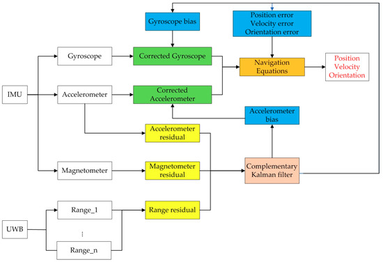
Figure 1. Algorithm block diagram.

CKF has three advantages [20,30,31]: first, there is no need to define a motion model, that is, the algorithm can be used for both vehicle and pedestrian applications. Secondly, the error of the state is stored rather than the state itself. When the system is linearized, it can be approximated by a smaller quantity, and a relatively more accurate result can be obtained. Finally, after each correction of the state value, it can be assumed that the current state is correct, that is, the error of the state value is reset to zero. In this way, in each prediction calculation of CKF, only the calculation of system covariance P is needed. In the update stage, the measurement matrix H can be simplified because the observation equation has no prior error.

The remainder of the paper is organized as follows: In Section 2, the fusion algorithm of UWB and IMU based on CKF is discussed, and the motion model and observation model of the algorithm are given. The uncertainty setting method of different observation values in the observation model is analyzed in detail. Subsequently, several experiments are analyzed in Section 3, and Section 4 concludes the paper.

2. Fusion Location Algorithm of IMU/UWB

2.1. State Model

Following the method in [32,33], the state of CKF algorithm is defined as follows: $X=[\delta p^n\delta v^n\epsilon b_g{b}_a$], where $\delta p^n$ is the position error, $\delta v^n$ is the velocity error, $\epsilon$ is the directional error, $b_g$ is the bias of the gyroscope, and $b_a$ is the bias of acceleration. $X$ is a 15-dimensional vector. The first three navigation state vectors are under the navigation coordinate system (n-frame), and the last two bias vectors are under body frame (b-frame). Before integrating the IMU data, the bias vector needs to be removed.

The differential equation of system dynamic model under continuous time is defined as follows:

$$\dot{X}=FX+W$$

(1)

$F$ is the state transition matrix and $W$ is the system noise. In order to facilitate the processing of EKF algorithm, the formula (1) is discretized into

$$X_{k+1}={\varnothing }_k{X}_k+W_k$$

(2)

$${\varnothing }_k=e^{F_{k}dt}$$

(3)

$F_k$ is the transition matrix at k time. In order to determine $F_k$, the transformation formula of state X must be derived.

2.1.1. The Equation of Acceleration and Gyroscope Bias

The measuring equations of acceleration and gyroscope are as follows:

$${\tilde{f}}^b=f^b+b_a+n_a$$

(4)

$${\tilde{\omega }}^b={\omega }^b+b_g+n_g$$

(5)

${\tilde{f}}^b$ and ${\tilde{\omega }}^b$ are the measured values of acceleration and gyroscope, $f^b$ and ${\omega }^b$ are the true values of acceleration and gyroscope, $n_a$ and $n_g$ are the measurement noise of the acceleration and the gyroscope, respectively, which satisfy the Gaussian distribution, and the covariance are defined as $N_a$,$N_g$, respectively. $b_a$ and $b_g$ are drift bias of the acceleration and the gyroscope, which are not a static value, but a time-dependent first-order Markov process, defined as follows:

$${\dot{b}}_a=-t_a{}^{-1}{b}_a+{\mu }_a$$

(6)

$${\dot{b}}_g=-t_g{}^{-1}{b}_g+{\mu }_g$$

(7)

${\mu }_a$ and ${\mu }_g$ are offset noise of the acceleration and the gyroscope, respectively, and satisfies Gaussian distribution, and the covariance are defined as $U_a$, $U_g$, respectively.

2.1.2. The Directional Error Equation

The directional error $\epsilon$ is caused by the gyro error and is defined as follows:

$$\dot{\epsilon }=C_b^n\delta {\omega }^b$$

(8)

$C_b^n$ represents the conversion from b-frame to n-frame, while $\delta {\omega }^b$ is the measurement error of the gyroscope, which is caused by drift bias and noise:

$$\delta {\omega }^b{b}_g+n_g$$

(9)

2.1.3. The Error Equation of Velocity and Position

The velocity error is caused by acceleration error and direction error, and is defined as:

$$\delta {\dot{v}}^n=\left[f^n\times \right]\epsilon +C_b^n\delta f^b$$

(10)

$\left[f^n\times \right]\epsilon$ represents the effect of directional error on acceleration, $\delta f^b$ is the measurement error of acceleration, which is caused by drift bias and noise and is defined as:

$$\delta f^b=b_a+n_a$$

(11)

The position error is defined as:

$$\delta {\dot{p}}^n=\delta {\mathrm{v}}^n$$

(12)

From the error equation, the state transition matrix $F$ of the system is deduced as follows:

$$F=\left[\begin{array}{c}0\\ 0\\ 0\\ 0\\ 0\end{array}\begin{array}{c}I\\ 0\\ 0\\ 0\\ 0\end{array}\begin{array}{c}0\\ \left[f^n\times \right]\\ 0\\ 0\\ 0\end{array}\begin{array}{c}0\\ 0\\ -C_b^n\\ diag\left(-{t_g}^{-1}\right)\\ 0\end{array}\begin{array}{c}0\\ C_b^n\\ 0\\ 0\\ diag\left(-{t_a}^{-1}\right)\end{array}\right]$$

(13)

The system noise $W$ is:

$$W=\left[\begin{array}{c}0\\ C_b^n{n}_a\\ -C_b^n{n}_g\\ {\mu }_a\\ {\mu }_g\end{array}\right]$$

(14)

The covariance matrix of system noise $W$ is:

$$Q=\left[\begin{array}{c}{N}_a\\ 0\\ 0\\ 0\end{array}\begin{array}{c}0\\ N_g\\ 0\\ 0\end{array}\begin{array}{c}0\\ 0\\ U_a\\ 0\end{array}\begin{array}{c}0\\ 0\\ 0\\ U_g\end{array}\right]$$

(15)

Define the noise transformation matrix as:

$$G=\left[\begin{array}{c}0\\ C_b^n\\ 0\\ 0\\ 0\end{array}\begin{array}{c}0\\ 0\\ -C_b^n\\ 0\\ 0\end{array}\begin{array}{c}0\\ 0\\ 0\\ I\\ 0\end{array}\begin{array}{c}0\\ 0\\ 0\\ 0\\ I\end{array}\right]$$

(16)

The noise covariance matrix is discretized to:

$$Q_k=\frac{1}{2}\left({\varnothing }_{k}GQ{G}^{\prime }+GQ{G}^{\prime }{\varnothing }_k{}^{\prime }\right)$$

(17)

Thus far, ${\varnothing }_k,Q_k$ in the prediction equation of CFK algorithm was defined, while ${\mathrm{Z}}_k$,${\mathrm{H}}_k,{\mathrm{R}}_k$ and other matrices were defined in Section 2.2.

2.2. The Observation Model

2.2.1. UWB Observations

There are $n$ base stations with known coordinates (four used in the experiment), $S_i=(S_{x,i}$, $S_{y,i}$, $S_{z,i})$, $i\in \left(1,n\right)$.

The observation function is defined as:

$$h\left(\delta {\widehat{p}}_k^n\right)=\left[\begin{array}{c}\Vert S_1-\left(\delta {\widehat{p}}_k^n+{\widehat{p}}_{ins,k}\right)\Vert -\Vert S_1-{\widehat{p}}_{ins,k}\Vert \\ ⋮\\ \Vert S_4-\left(\delta {\widehat{p}}_k^n+{\widehat{p}}_{ins,k}\right)\Vert -\Vert S_4-{\widehat{p}}_{ins,k}\Vert \end{array}\right]$$

(18)

where ${\widehat{p}}_{ins,k}=\left({\widehat{x}}_k,{\widehat{y}}_k,{\widehat{z}}_k\right)$ represents the position coordinates calculated by INS. $\delta {\widehat{p}}_k^n=\left(\delta {\widehat{x}}_k,\delta {\widehat{y}}_k,\delta {\widehat{z}}_k\right)$ represents a priori position error calculated by the state transition equation. $\Vert .\Vert$ represents the Euclidean distance. The formula (18) represents the difference between the ranging value after considering the position error and the ranging value from the INS integral position without considering the position error to the base station. The Jacobian matrix of the observation equation is defined as follows:

$${\mathrm{H}}_k=\frac{\delta \left(h\left(\delta {\widehat{p}}_k^n\right)\right)}{\delta \left(\delta {\widehat{p}}_k^n\right)}=\left[\begin{array}{c}\frac{S_{x1}-({\widehat{x}}_k+\delta {\widehat{x}}_k)}{\Vert S_1-(\delta {\widehat{p}}_k^n+{\widehat{p}}_{ins,k})\Vert }\\ ⋮\\ \frac{S_{x4}-({\widehat{x}}_k+\delta {\widehat{x}}_k)}{\Vert S_4-(\delta {\widehat{p}}_k^n+{\widehat{p}}_{ins,k})\Vert }\end{array}\begin{array}{c}\frac{S_{y1}-({\widehat{y}}_k+\delta {\widehat{y}}_k)}{\Vert S_1-(\delta {\widehat{p}}_k^n+{\widehat{p}}_{ins,k})\Vert }\\ ⋮\\ \frac{S_{y4}-({\widehat{y}}_k+\delta {\widehat{y}}_k)}{\Vert S_4-(\delta {\widehat{p}}_k^n+{\widehat{p}}_{ins,k})\Vert }\end{array}\begin{array}{c}\frac{S_{z1}-({\widehat{z}}_k+\delta {\widehat{z}}_k)}{\Vert S_1-(\delta {\widehat{p}}_k^n+{\widehat{p}}_{ins,k})\Vert }\\ ⋮\\ \frac{S_{z4}-({\widehat{z}}_k+\delta {\widehat{z}}_k)}{\Vert S_4-(\delta {\widehat{p}}_k^n+{\widehat{p}}_{ins,k})\Vert }\end{array}\begin{array}{c}{0}_{1\times 12}\\ ⋮\\ 0_{1\times 12}\end{array}\right]$$

(19)

Observations are defined as:

$${\mathrm{Z}}_{k,i}={\mathrm{r}}_{k,i}-\Vert S_i-{\widehat{p}}_{ins,k}\Vert$$

(20)

${\mathrm{r}}_k$ is the ranging data of UWB. The formula (20) represents the distance difference between the ranging data of the UWB and the distance to the base station calculated from the INS position.

The standard observation equation is defined as follows:

$${\mathrm{Z}}_k={\mathrm{H}}_k{\mathrm{X}}_k+{\mathrm{V}}_k$$

(21)

${\mathrm{V}}_k$ is the measurement noise matrix, ${\mathrm{V}}_k~N\left(0,{\mathrm{R}}_k\right)$.

For UWB data, the accuracy of UWB sensor observations may be affected by ambient temperature, power supply stability, fixed obstacles, and even people or objects moving in the positioning scene. Therefore, it is necessary to estimate the confidence of UWB observations. A correlation method based on UWB positioning residual is designed.

In order to simplify the description, there are three base stations, and in the plane location, it is assumed that the UWB base station with the coding number i is recorded as ${\mathrm{Beacon}}_{\mathrm{i}}$, and its seat is marked $\left(x_{\mathrm{i}},y_{\mathrm{i}}\right)$. The UWB tag used for positioning is marked tag, and its seat is marked $\left(x,y\right)$. The real distance between tag and ${\mathrm{Beacon}}_{\mathrm{i}}$ is recorded as ${\mathrm{r}}_{\mathrm{i}}$, and the measured value of this distance is recorded as ${\mathrm{r}}_{\mathrm{i}}^{\prime }$. As Figure 2 shows, ideally, $r_i^{\prime }=r_i$, where the only point can be determined by the intersection of three circles, is the location of the tag under the current observation data. In order to obtain the solution of this point, an error function is defined, and the coordinates of tag are obtained by minimizing the error function. One possible error function is:

$$E\left(x,y\right)={{\displaystyle \sum }}_i^{n}abs\left(\sqrt{\left({\left(x-x_i\right)}^2+{\left(y-y_i\right)}^2\right)}-r_i^{\prime }\right)$$

(22)

where, abs() represents an absolute function. The coordinates $\left(x\prime ,y\prime \right)$ can be obtained by minimizing $E\left(x,y\right)$, that is:

$$\left(x\prime ,y\prime \right)=argmi{n}_{\left(x,y\right)}E\left(x,y\right)$$

(23)

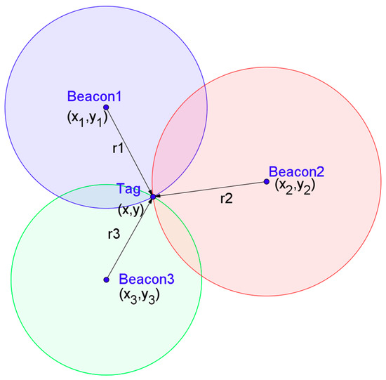
Figure 2. Schematic diagram of trilateral positioning.

Ideally, the minimum value of $E\left(x,y\right)$ is 0. However, in practical application, the measured value often has a certain deviation. Suppose $r_i$ still represents the real distance, and the deviation of $r_i$ is recorded as $\Delta r_i$. At this point, the measured value of the corresponding ${\mathrm{Beacon}}_i$ is $r_i^{\prime }=r_i+\Delta r_i$. Figure 3 shows the area where the circles represented by the three beacon measurements around the tag intersect. In the case of errors in the measurements, the three circles do not intersect at one point, but intersect in pairs. In this case, the estimate of the tag coordinates $\left(x^{\prime },y^{\prime }\right)$ is still obtained by minimizing $E\left(x,y\right)$. Generally speaking, when the error of $r_i^{\prime }$ is large, the value of $\Delta r_i$ is also larger.

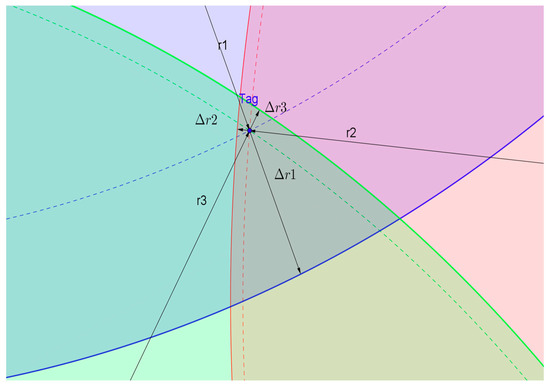
Figure 3. Local schematic diagram of non-line-of-sight (NLOS) trilateral positioning.

The uncertainty for defining UWB data is as follows:

$$C_{ui}=\max ({\alpha }_u{e}^{\Delta r_i},C_{u\_max})$$

(24)

${\mathrm{C}}_{\mathrm{ui}}\in [0,+\infty$], $\mathrm{i}\in \left[1,\mathrm{n}\right]$. The value of ${\mathsf{\alpha }}_{\mathrm{u}}$ is a constant, which is an estimate of the overall residual value and indicates the degree of distrust in the original UWB data. When the value of ${\mathsf{\alpha }}_{\mathrm{u}}$ or ${\Delta \mathrm{r}}_{\mathrm{i}}$ is higher, the more unreliable the data is. ${\mathrm{C}}_{\mathrm{u}\_\max }$ is to limit the value of ${\mathrm{C}}_{\mathrm{ui}}$ in a certain range, otherwise it is easy to appear singular matrix. The measurement noise matrix ${\mathrm{R}}_{\mathrm{k}}$ of UWB is defined as follows:

$${\mathrm{R}}_k=\left[\begin{array}{c}{\sigma }_{s1}^2{C}_{u1}\\ 0\\ 0\\ 0\end{array}\begin{array}{c}0\\ {\sigma }_{s2}^2{C}_{u2}\\ 0\\ 0\end{array}\begin{array}{c}0\\ 0\\ {\sigma }_{s3}^2{C}_{u3}\\ 0\end{array}\begin{array}{c}0\\ 0\\ 0\\ {\sigma }_{s4}^2{C}_{u4}\end{array}\right]$$

(25)

${\sigma }_{si}^2$ represents the covariance of the ranging value from the No.i UWB base station to the tag. If there are less than three values in the ranging data due to occlusion and other reasons, the effective residual cannot be obtained. In the experiment, if the sum of the two ranging values is greater than the distance between the two base stations, the residual is 0, and $C_u={\alpha }_u$. The range values that are obscured and cannot be obtained should be removed from the corresponding rows in ${\mathrm{R}}_k$ and ${\mathrm{Z}}_k$.

2.2.2. Observations of Accelerometers and Magnetometers

The error observations of accelerometers and magnetometers are defined as follows:

$$\delta f^n=C_b^n{\widehat{f}}^b-g^n$$

(26)

$$\delta m^n=C_b^n{\widehat{m}}^b-m^n$$

(27)

${\widehat{f}}^b$ and ${\widehat{m}}^b$ are offset compensated measurements, respectively.$g^n$ and $m^n$ are the standard values of gravity acceleration and geomagnetic field in the navigation system.

The observation vector is defined as:

$${\mathrm{Z}}_k=\left[\delta f^b,\delta m^b\right]$$

(28)

The observation equation is defined as follows:

$${\mathrm{Z}}_k={\mathrm{H}}_k{\mathrm{X}}_k+{\mathrm{V}}_k$$

(29)

The observation model matrix ${\mathrm{H}}_k$ is defined as follows:

$${\mathrm{H}}_k=\left[\begin{array}{c}I\\ 0\\ 0\end{array}\begin{array}{c}0\\ 0\\ 0\end{array}\begin{array}{c}0\\ C_n^b\left[g^n\times \right]\\ C_n^b\left[m^n\times \right]\end{array}\begin{array}{c}0\\ 0\\ 0\end{array}\begin{array}{c}0\\ 0\\ 0\end{array}\right]$$

(30)

${\mathrm{V}}_k$ is the measurement noise matrix, ${\mathrm{V}}_k~N\left(0,{\mathrm{R}}_k\right)$. In general, the measurement noise covariance matrix ${\mathrm{R}}_k$ is constant, but in fact, ${\mathrm{R}}_k$ is closely related to the specific sensor application environment. For gravity data, pitch and roll angle can be estimated. On the other hand, the geomagnetic data can be used to estimate the yaw angle. However in fact, body acceleration cannot be neglected with comparison to gravity, and the geomagnetic data will also have disturbance, which will affect the accuracy of the direction correction. In order to reduce the influence of the direction calculation of the noise data, a method based on dynamic ${\mathrm{R}}_k$ matrix is designed.

The magnitude residual (${\mathrm{E}}_m^m$) of the magnetometer and the magnitude residual (${\mathrm{E}}_g^m$) of the gravity acceleration are defined as follows:

$${\mathrm{E}}_m^m=\max \left(\frac{\Vert {\widehat{m}}^b\Vert }{\Vert m^n\Vert },\frac{\Vert m^n\Vert }{\Vert {\widehat{m}}^b\Vert }\right)$$

(31)

$${\mathrm{E}}_g^m=\max \left(\frac{\Vert {\widehat{f}}^b\Vert }{\Vert g^n\Vert },\frac{\Vert g^n\Vert }{\Vert {\widehat{f}}^b\Vert }\right)$$

(32)

$\Vert .\Vert$ is taken as the normal value. Both ${\mathrm{E}}_m^m$ and ${\mathrm{E}}_g^m$ $\in [1,+\infty$], which represent the degree of deviations of the measured values ${\widehat{m}}^b$ and ${\widehat{f}}^b$ from the standard values $m^n$ and $g^n$ on magnitude. The direction residual (${\mathrm{E}}_m^d$) of the magnetometer and the direction residual (${\mathrm{E}}_g^d$) of the gravity acceleration are also defined as follows:

$${\mathrm{E}}_m^d=\Vert \frac{{\widehat{m}}^b}{\Vert {\widehat{m}}^b\Vert }-\frac{m^n}{\Vert m^n\Vert }\Vert$$

(33)

$${\mathrm{E}}_g^d=\Vert \frac{{\widehat{f}}^b}{\Vert {\widehat{f}}^b\Vert }-\frac{g^n}{\Vert g^n\Vert }\Vert$$

(34)

Both ${\mathrm{E}}_m^d$ and ${\mathrm{E}}_g^d\in [0,+\infty$]. Define the uncertainty of the magnetometer and acceleration data as follows:

$$C_m=\max (e^{{\alpha }_m{\mathrm{E}}_m^m{\mathrm{E}}_m^d},C_{m\_max})$$

(35)

$$C_g=\max (e^{{\alpha }_g{\mathrm{E}}_g^m{\mathrm{E}}_g^d},C_{g\_max})$$

(36)

Both $C_m$ and $C_g\in [0,+\infty$]. $C_{m\_max}$ and $C_{g\_max}$ are to limit the values of $C_m$ and $C_g$ in a certain range, otherwise singular matrices are easy to appear. Both ${\alpha }_m$ and ${\alpha }_g$ are greater than zero, indicating the degree of distrust in the original data of the magnetometer and the acceleration. The greater value of $\alpha$ or $\mathrm{E}$, the less reliable the data is. Finally, the mean of ${\mathrm{R}}_k$ is defined as follows:

$${\mathrm{R}}_k=\left[\begin{array}{cc}{\sigma }_f^2{C}_g& 0\\ 0& {\sigma }_m^2{C}_m\end{array}\right]$$

(37)

${\sigma }_f^2,{\sigma }_m^2$ represent the covariance of the acceleration and magnetometer measurements, respectively.

2.3. INS Navigation Equation

Through the integration of gyroscope and acceleration data, the direction, velocity, position, and other data under the navigation system can be obtained. The INS navigation equation is defined as follows:

$${\dot{p}}^n=v^n$$

(38)

$${\dot{v}}^n=v^n{C}_b^n{f}^b+g^n$$

(39)

$${\dot{C}}_b^n=C_b^n[{\omega }^b\times ]$$

(40)

${\mathrm{g}}^{\mathrm{n}}$ is the gravity vector under n-frame, ${\mathrm{f}}^{\mathrm{b}}$ is the acceleration vector under b-frame, ${\mathsf{\omega }}^{\mathrm{b}}=[{\mathsf{\omega }}_{\mathrm{x}}^{\mathrm{b}}$,${\mathsf{\omega }}_{\mathrm{y}}^{\mathrm{b}},{\mathsf{\omega }}_{\mathrm{z}}^{\mathrm{b}}]$ is the angular velocity under b-frame, and $[{\mathsf{\omega }}^{\mathrm{b}}\times ]$ is the skew-symmetric matrix of the angular velocity, as follows:

$$[{\omega }^b\times ]=\left[\begin{array}{ccc}0& -{\omega }_z^b& {\omega }_y^b\\ {\omega }_z^b& 0& -{\omega }_x^b\\ -{\omega }_y^b& {\omega }_x^b& 0\end{array}\right]$$

(41)

For acceleration and gyroscope observations at k time, the offset value calculated by the CKF algorithm is first removed), as follows:

$${\widehat{f}}_k^b={\tilde{f}}_k^b-b_a$$

(42)

$${\widehat{\omega }}_k^b={\tilde{\omega }}_k^b-b_g$$

(43)

${\tilde{f}}_k^b$ and ${\tilde{\omega }}_k^b$ represent the original observations of the acceleration and angular velocity, and ${\widehat{f}}_k^b$ and ${\widehat{\omega }}_k^b$ represent the offset compensated values.

The transformation of acceleration from k time to k+1 time is as follows:

$${\widehat{f}}_{k+1}^n=C_b^n\left({\tilde{f}}_k^b+0.5({\tilde{\omega }}_k^b{d}_t\otimes {\tilde{f}}_k^b)\right)-g^n$$

(44)

⊗ represents the vector cross multiplication and the rotation correction of the acceleration caused by the change of angular velocity.

The transformation of the speed from the k time to the k+1 time is as follows:

$$v_{k+1}^n=v_k^n+{\widehat{f}}_{k+1}^n{d}_t-\delta v_k^n$$

(45)

$\delta v_k^n$ represents the error of the velocity at k time, which is cyclically calculated by the CKF algorithm.

The change of position from k time to k+1 time is as follows:

$$p_{k+1}^n=p_k^n+0.5(v_k^n+v_{k+1}^n)d_t-\delta p_k^n$$

(46)

$\delta p_k^n$ represents the error of the position at k time, which is cyclically calculated by the CKF algorithm.

The change of posture from k time to k+1 time is as follows:

$$C_{b,\mathrm{k}+1}^n\prime =(\mathrm{I}-\left[\epsilon \times \right])C_{b,\mathrm{k}}^n$$

(47)

$$C_{b,\mathrm{k}+1}^n=C_{b,\mathrm{k}+1}^n\prime (\mathrm{I}+\left[{\tilde{\omega }}_k^b{d}_t\times \right])$$

(48)

The value of $C_{b,\mathrm{k}+1}^n{}^{\prime }$ represents the result of correcting the orientation error of the pose change matrix $C_{b,\mathrm{k}}^n$ at k time, and the error $\epsilon$ is calculated cyclically by CKF algorithm. Then, for $C_{b,\mathrm{k}+1}^n\prime$, the rotation compensation, from k time to k + 1 time is carried out to obtain the rotation matrix $C_{b,\mathrm{k}+1}^n$. In order to improve the accuracy of attitude values, the value of $C_{b,\mathrm{k}+1}^n$ requires periodic normalization.

3. Experiment

A test site is set up in the underground garage of a university. As shown in Figure 4, four UWB base stations are placed on four corners of the rectangular area. The IMU device chose X-IMU from X-IO company in the UK. The core chip of UWB tag/base station is DWM1000 chip of Decawave Company. The UWB tag is fixed to the car. At the same time, the IMU is fixed 5 cm below the UWB tag. In order to keep the data of IMU and UWB synchronized, the notebook in the car receives ranging data from IMU and UWB at the same time. In the process of clockwise movement, the car basically maintains a uniform speed.

Figure 4. Route 1.

The experiment set two routes, one is a rectangular route with fewer turns, and the other is an eight-shaped route with more turns, such as route 1 and route 2 in Figure 4 and Figure 5. The locations of the four base stations are shown in the rectangular points, and the two red circles in the figure represent the two columns in the underground garage. Because the real trajectory of the car motion cannot be obtained, this trajectory is only used as a reference schematic diagram. In addition, in order to increase the location noise of the eight-shaped route, one to two base stations will be blocked randomly, which will cause the ranging data to be abnormal or data loss.

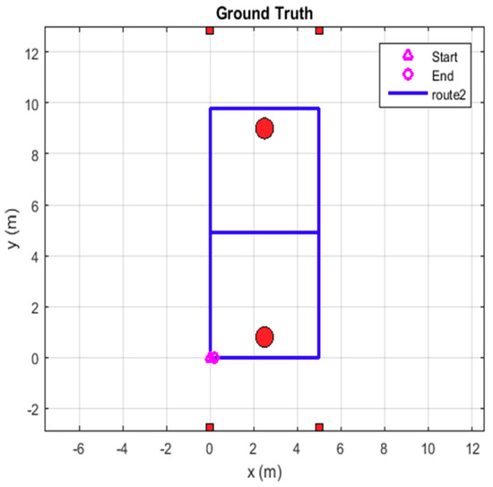
Figure 5. Route 2.

In the experimental analysis, first of all, the positioning results are analyzed. Then the influence on the positioning results is analyzed from different types of observations, such as geomagnetic residual, gravity residual, ranging residual and so on.

3.1. Analysis of Location Results of Route 1

3.1.1. Positioning Trajectory Analysis

The location result of path 1 is given in Figure 6. The left figure is the location result given by the optimization algorithm. In general, with the exception of a few points deviating from the overall trajectory, the rest of the anchor points are aggregated on the path of the car motion. The right image shows the trajectory of the fusion of UWB and IMU. It can be seen that the fusion trajectory gives a higher frequency of positioning results, and provides attitude information for each positioning result. Compared with the left image, the track of the right image is smoother.

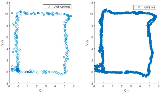
Figure 6. Positioning results in path 1.

The main state of the fusion algorithm is shown in Figure 7. From top to bottom, they are the bias of the acceleration, the bias of the gyroscope, the change of velocity, and angle in turn. Because the residual of UWB ranging data is relatively small, the integral drift of INS is well constrained, and the bias of velocity and acceleration is effectively modified. As can be seen from subfigure 3 of Figure 7, the speed value is basically about ±1 meter, which is consistent with the actual value. As can be seen from subfigure 4 of Figure 7, through the correction of the opposite direction value of the magnetometer and accelerometer, the bias of the gyroscope can be estimated effectively. In addition, the angle change of the trolley movement on path 1 is relatively regular, and the angle value is close to the actual value. Subfigures 1 and 2 are bias values estimated from position and angle updates, which are subtracted from each integral of the accelerometer and gyroscope.

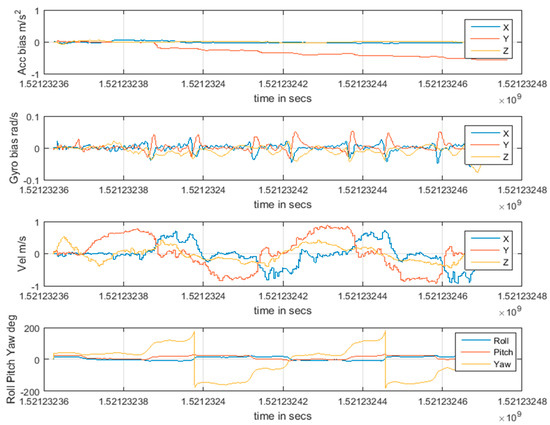
Figure 7. Main state variables of fusion algorithm.

3.1.2. Analysis of Geomagnetism and Gravity Residual

From the above figure, it can be seen that the magnetic field data in the whole path 1 is relatively stable, and the geomagnetism changes regular with the attitude change of the trolley in two consecutive circles. Initially, the car stood still. The geomagnetic data for a period of time (5 to 10 seconds) are collected and converted to n-frame as the environmental standard geomagnetic data ($m^n$ in the second part of Section 2.2). If there is no geomagnetic interference in the environment, all subsequent geomagnetic data should be equal to the standard geomagnetic data after they are converted to n-frame. On this basis, the transformation matrix $C_b^n$ from b-frame to n-frame in the whole process of motion can be obtained.

The bottom figure in Figure 8 shows the difference between the magnetometer data converted to n-frame and the environmental standard geomagnetic data $m^n$, which should ideally be zero. The non-zero value in the graph comes from the influence of two cases: one is that the geomagnetism in the environment is unstable; the other is that the calculation of the transformation matrix $C_b^n$ itself is not completely accurate. However, due to the relatively small error, it can be seen from Table 1 that the average geomagnetic error is not more than 0.2 g. Therefore, it is theoretically feasible to calculate the direction of geomagnetism in this environment.

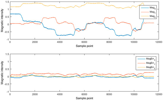
Figure 8. Magnetic field and its residual data in path 1.

Table 1. Geomagnetic residual in path 1 (Gauss).

Coordinate Axis	Average of Absolute Value	Max	Min
X	0.0449	0.1188	−0.1180
Y	0.1564	0.2720	−0.0125
Z	0.0287	0.0839	−0.0783

For gravity data, similar to magnetometer data, accelerometer data collected for an initial rest period (5 to 10 seconds) are converted to n-frame as environmental standard gravity data ($g^n$ in the second part of Section 2.2). If the interference of acceleration in the motion of the car is ignored, all subsequent accelerometer data should be equal to the standard gravity data converted to n-frame. On this basis, the transformation matrix $C_b^n$ from b-frame to n-frame in the whole process of motion can be obtained.

As shown in Figure 9, the above figure shows the acceleration data for path 1, and the following figure shows the difference between the accelerometer data converted to n-frame and the standard gravity data $g^n$, which should ideally be zero. The non-zero value in the graph comes from the influence of two cases: one is that the motion of the trolley is actually non-uniform and moving under the acceleration caused by the periodic pulling force; the other is that the calculation of the transformation matrix $C_b^n$ itself is not completely accurate. As can be seen from Table 2, the error between X- and Z-axis is relatively small, and the average gravity residual is less than 0.8 G. The average gravity residual of the Y-axis is about 2 G, which explains why the acceleration residual of the Y-axis is increasing in subfigure 1 of Figure 7. Generally speaking, the calculation of gravity constraint direction in this environment is still feasible in theory, but its confidence is lower than that of geomagnetic data.

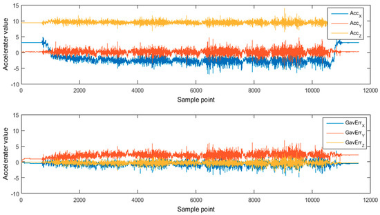
Figure 9. Acceleration and gravity residual data in path 1.

Table 2. Gravity residual data in path 1 (m/s²).

Axial Direction	Average of Absolute Value	Max	Min
X	0.7248	4.8814	−3.7402
Y	2.0226	6.0312	−1.5509
Z	0.6095	3.4986	−3.4159

3.1.3. Residual Analysis of UWB Data

As can be seen in Figure 10, the UWB ranging data of route 1 is partially obscured by the column, resulting in a state of discontinuity. The corresponding $\Delta r_i$ is shown in Figure 11. The columns of different colors represent the ranging residual value of the corresponding base station respectively. As can be seen from Figure 10, the ranging value is relatively unstable at several peaks, because the ranging error of UWB increases with the increase of distance. In Figure 11, the ranging residual increases accordingly. By analyzing the proportion of ranging residual, the weight of covariance of observation values of different base stations is determined dynamically. As can be seen from Table 3, the average ranging residual of the four base stations is less than 0.1 meters, indicating that the overall quality of path 1 is high. The minimum residual value of 0 indicates that the ranging value is obscured at a certain time, and the residual error is not calculated at this time.

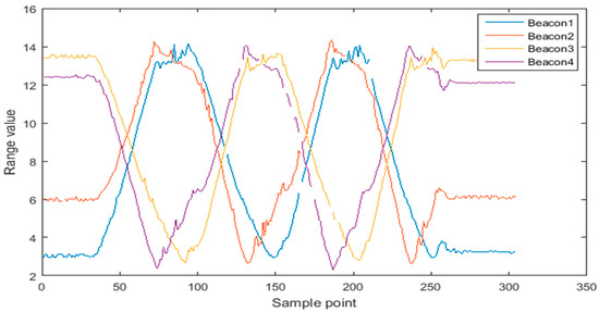
Figure 10. Ranging data in path 1.

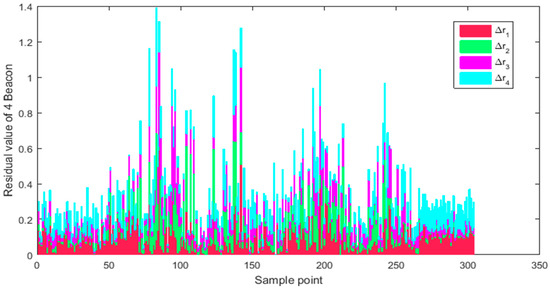
Figure 11. Ultra-wideband (UWB) ranging residual data in path 1.

Table 3. Ranging residual data in path 1 (m).

Base Station	Average of Absolute Value	Max	Min
Beacon1	0.0910	0.5882	0
Beacon2	0.0733	0.6012	0
Beacon3	0.0688	0.5283	0
Beacon4	0.0919	0.4413	0

3.2. Analysis of Location Trajectory of Route 2

3.2.1. Location Trajectory Analysis

The location result of path 2 is given in Figure 12, and the left figure is the location result given by the optimization algorithm. Because more positions on path 2 are blocked by stone columns, coupled with the human interference of the testers, there are many of anomalies that deviate from the trajectory. The right image is the trajectory of UWB and IMU fusion, it can be seen that the fusion track gives a higher frequency positioning results, compared with the left image, the right trajectory effectively shielded the abnormal points of the left image, and the trajectory is smoother.

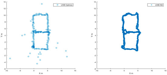
Figure 12. Positioning results in path 2.

3.2.2. Analysis of Geomagnetism and Gravity Residual

The blue data in Figure 13 is the residual modulus value of gravity data $\Vert \delta f^n\Vert$, and the corresponding red data is the uncertainty $C_g$ of gravity residual data. The blue data in Figure 14 is the residual modulus value of the geomagnetic data $\Vert \delta m^n\Vert$, which corresponds to the uncertainty $C_m$ of the geomagnetic residual data.

Figure 13. Comparison of uncertainty and residual value of gravity data in path 2.

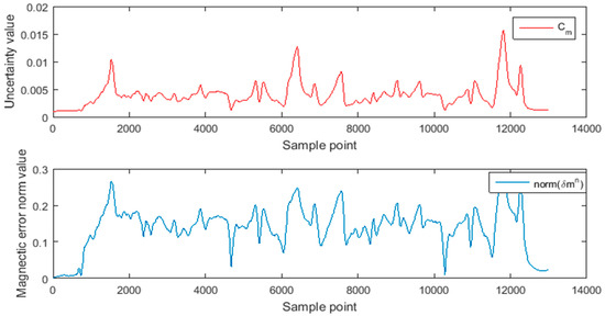
Figure 14. Comparison of uncertainty and residual value of geomagnetic data in path 2.

The residual of the magnetic field data and gravity data in the whole path 2 are basically consistent with the uncertainty of setting, which shows that the given uncertainty formula and parameters can well reflect the residual variation of geomagnetism and gravity data. Thus, in the process of filtering, we can intervene the covariance of the observed values in order to obtain a more accurate direction value. The correction and update of the direction value further restrict the bias of the gyroscope. Figure 15 is a comparison of the effects of $C_{\mathrm{g}}$ and $C_m$ on gyroscope data. It can be seen that under the condition of uncertainty intervention, the bias error of the gyroscope is almost twice as small, thus improving the accuracy of angle estimation.

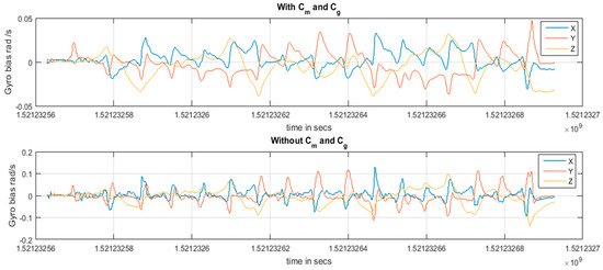
Figure 15. Bias comparison of gyroscopes with and without uncertainty in path 2.

3.2.3. Residual Analysis of UWB Data

As can be seen in Figure 16, the UWB ranging value of route 2 has changed greatly at some time due to the occlusion of stone columns and human interference. The corresponding $\Delta r_i$ is shown in Figure 17, and the optimal residual also increases at the ranging jump point. As can be seen from Table 4, although the average ranging residual of the four base stations is about 0.2 m, the highest residual value is more than two meters, which will cause the outlier with large positioning deviation. By dynamically increasing the covariance of ranging outliers, the influence of anomalies on the fusion algorithm can be shielded.

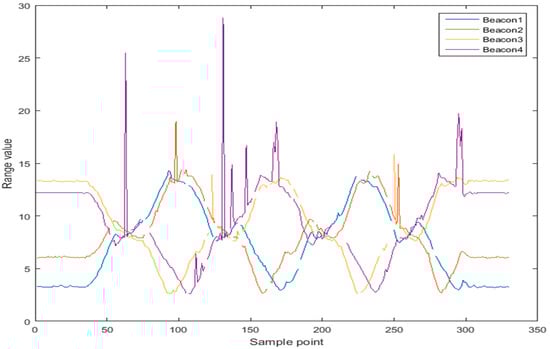
Figure 16. Comparison of uncertainty and error of geomagnetic data in path 2.

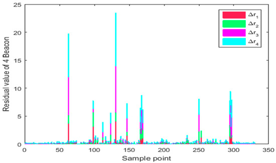
Figure 17. UWB ranging residual data in path 2.

Table 4. Ringing residual in route 2 (m).

Base Station	Average of Absolute Value	Max	Min
Beacon1	0.1362	4.0561	0
Beacon2	0.1400	2.5900	0
Beacon3	0.1781	8.2678	0
Beacon4	0.2304	9.5135	0

As can be seen from Figure 18, the sample points with large residual errors in Figure 17 also have greater uncertainty values in Figure 18. That is, Figure 18 exponentially magnifies the residual in Figure 17 to increase the sensitivity to the residual data.

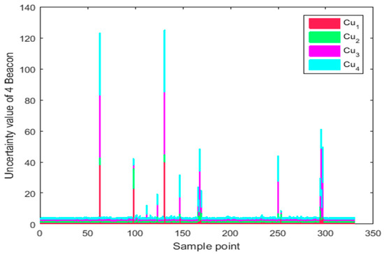
Figure 18. Uncertainty of UWB residual data in path 2.

Generally speaking, the fusion algorithm can dynamically give the corresponding confidence according to the gravity residual, geomagnetism residual and ranging residual in route 1 and 2, so as to evaluate the observed values effectively and improve the accuracy and robustness of the fusion algorithm.

4. Conclusions

In this paper, a fusion location method of UWB and IMU based on adaptive CKF is presented. The algorithm optimizes the location results by adaptively setting the weights of UWB data, magnetic field data, and acceleration data and so on. Firstly, through the analysis of UWB ranging data, it can be seen that in non-line-of-sight environment, the accuracy of UWB ranging will be affected. However, by dynamically increasing the covariance of ranging outliers, the influence of anomalies on the fusion algorithm can be shielded. Secondly, with the analysis of geomagnetic and gravity data in the experimental scene, the residual of geomagnetic and gravity data is small, which can meet the needs of heading calculation. However, the credibility of geomagnetic data is better than that of gravity data. Then, the fusion of UWB and IMU not only can eliminate the multi-path and non-line-of-sight effect caused by occlusion of UWB signal, but also restricts the drift of INS, corrects the deviation of velocity and acceleration, and realizes the complementary advantages. However, there are two good prerequisites in the experiment. That is, the motion of the car is relatively stable and the experimental geomagnetic data are relatively stable. Thus, in the face of more complex motion patterns such as rapid acceleration and stop, as well as more and stronger geomagnetic interference environment, better motion models and algorithms need to be studied and further tested.

References

- Xin, L.; Jian, W.; Liu, C.; Zhang, L.; Li, Z. Integrated WiFi/PDR/Smartphone Using an Adaptive System Noise Extended Kalman Filter Algorithm for Indoor Localization. Int. J. Geo-Inf. 2016, 5, 8. [Google Scholar]
- Santoso, F.; Redmond, S.J. Indoor location-aware medical systems for smart homecare and telehealth monitoring: State-of-the-art. Physiol. Meas. 2015, 36, R53–R87. [Google Scholar] [CrossRef] [PubMed]
- Liu, F.; Wang, J.; Zhang, J.; Han, H. An Indoor Localization Method for Pedestrians Base on Combined UWB/PDR/Floor Map. Sensors 2019, 19, 2578. [Google Scholar] [CrossRef] [PubMed]
- Dabove, P.; Di Pietra, V.; Piras, M.; Jabbar, A.A.; Kazim, S.A. Indoor positioning using Ultra-wide band (UWB) technologies: Positioning accuracies and sensors’ performances. In Proceedings of the 2018 IEEE/ION Position, Location and Navigation Symposium (PLANS), Monterey, CA, USA, 23–26 April 2018; pp. 175–184. [Google Scholar]
- García, E.; Poudereux, P.; Hernández, Á.; Ureña, J.; Gualda, D. A robust UWB indoor positioning system for highly complex environments. In Proceedings of the 2015 IEEE International Conference on Industrial Technology (ICIT), Seville, Spain, 17–19 March 2015; pp. 3386–3391. [Google Scholar]
- Zhang, J.; Shen, C. Research on UWB indoor positioning in combination with TDOA improved algorithm and Kalman filtering. Mod. Electron. Tech. 2016, 39, 1–5. [Google Scholar]
- Fan, Q.; Sun, B.; Yan, S.; Zhuang, X.J.I.S.J. Performance Enhancement of MEMS-Based INS/UWB Integration for Indoor Navigation Applications. IEEE Sens. J. 2017, 17, 3116–3130. [Google Scholar] [CrossRef]
- Denis, B.; Keignart, J.; Daniele, N. Impact of NLOS propagation upon ranging precision in UWB systems. In Proceedings of the IEEE Conference on Ultra Wideband Systems and Technologies, Reston, VA, USA, 16–19 November 2003; pp. 379–383. [Google Scholar]
- Wang, X.; Wang, Z.; O’Dea, B. A TOA-based location algorithm reducing the errors due to non-line-of-sight (NLOS) propagation. IEEE Trans. Veh. Technol. 2003, 52, 112–116. [Google Scholar] [CrossRef]
- Guvenc, I.; Chong, C.C. A survey on TOA based wireless localization and NLOS mitigation techniques. IEEE Commun. Surv. Tutor. 2009, 11, 107–124. [Google Scholar] [CrossRef]
- Mäkelä, M.; Kirkko-Jaakkola, M.; Rantanen, J.; Ruotsalainen, L. Proof of Concept Tests on Cooperative Tactical Pedestrian Indoor Navigation. In Proceedings of the 2018 21st International Conference on Information Fusion (FUSION), Cambridge, UK, 10–13 July 2018; pp. 1369–1376. [Google Scholar]
- Sczyslo, S.; Schroeder, J.; Galler, S.; Kaiser, T. Hybrid localization using UWB and inertial sensors. In Proceedings of the IEEE International Conference on Ultra-Wideband, Hannover, Germany, 10–12 September 2008. [Google Scholar]
- Yuan, X.; Chen, X.; Jin, C.; Zhao, Q.; Wang, Y. Improving tightly-coupled model for indoor pedestrian navigation using foot-mounted IMU and UWB measurements. In Proceedings of the Instrumentation & Measurement Technology Conference, Taipei, Taiwan, 23–26 May 2016. [Google Scholar]
- Fan, Q.; Sun, B.; Yan, S.; Wu, Y.; Zhuang, X. Data Fusion for Indoor Mobile Robot Positioning Based on Tightly Coupled INS/UWB. J. Navig. 2017, 70, 1079–1097. [Google Scholar] [CrossRef]
- Xu, Y.; Chen, X. Range-only uwb/ins tightly integrated navigation method for indoor pedestrian. Chin. J. Sci. Instrum. 2016, 37, 142–148. [Google Scholar]
- Wang, J.; Yang, G.; Li, Z.; Meng, X.; Hancock, C.M. A Tightly-Coupled GPS/INS/UWB Cooperative Positioning Sensors System Supported by V2I Communication. Sensors 2016, 16, 944. [Google Scholar] [CrossRef] [PubMed]
- Benini, A.; Mancini, A.; Longhi, S. An IMU/UWB/Vision-based Extended Kalman Filter for Mini-UAV Localization in Indoor Environment using 802.15.4a Wireless Sensor Network. J. Intell. Robot. Syst. 2013, 70, 461–476. [Google Scholar] [CrossRef]
- Li, K.; Wang, C.; Huang, S.; Liang, G.; Wu, X.; Liao, Y. Self-positioning for UAV indoor navigation based on 3D laser scanner, UWB and INS. In Proceedings of the 2016 IEEE International Conference on Information and Automation (ICIA), Ningbo, China, 1–3 August 2016; pp. 498–503. [Google Scholar]
- González, J.; Blanco, J.L. Mobile robot localization based on Ultra-Wide-Band ranging: A particle filter approach. Robot. Auton. Syst. 2009, 57, 496–507. [Google Scholar] [CrossRef]
- Zwirello, L.; Ascher, C.; Trommer, G.F.; Zwick, T. Study on UWB/INS integration techniques. In Proceedings of the Positioning Navigation & Communication, Dresden, Germany, 7–8 April 2011. [Google Scholar]
- Chen, P.; Kuang, Y.; Chen, X. A UWB/Improved PDR Integration Algorithm Applied to Dynamic Indoor Positioning for Pedestrians. Sensors 2017, 17, 2065. [Google Scholar] [CrossRef] [PubMed]
- Xu, Y.; Ahn, C.K.; Shmaliy, Y.S.; Chen, X.; Li, Y. Adaptive robust INS/UWB-integrated human tracking using UFIR filter bank. Measurement 2018, 123, 1–7. [Google Scholar] [CrossRef]
- Hartmann, F.; Rifat, D.; Stork, W. Hybrid indoor pedestrian navigation combining an INS and a spatial non-uniform UWB-network. In Proceedings of the 2016 19th International Conference on Information Fusion, Heidelberg, Germany, 5–8 July 2016; pp. 549–556. [Google Scholar]
- Hol, J.D.; Dijkstra, F.; Luinge, H.; Schon, T.B. Tightly coupled UWB/IMU pose estimation. In Proceedings of the IEEE International Conference on Ultra-Wideband, Vancouver, BC, Canada, 9–11 September 2009. [Google Scholar]
- Savioli, A.; Goldoni, E.; Savazzi, P.; Gamba, P. Low Complexity Indoor Localization in Wireless Sensor Networks by UWB and Inertial Data Fusion. Comput. Sci. 2013, 52, 723–732. [Google Scholar]
- Ascher, C.; Zwirello, L.; Zwick, T.; Trommer, G. Integrity monitoring for UWB/INS tightly coupled pedestrian indoor scenarios. In Proceedings of the International Conference on Indoor Positioning & Indoor Navigation, Guimaraes, Portugal, 21–23 September 2011. [Google Scholar]
- Fan, Q.; Wu, Y.; Hui, J.; Wu, L.; Yu, Z.; Zhou, L. Integrated navigation fusion strategy of INS/UWB for indoor carrier attitude angle and position synchronous tracking. Sci. World J. 2014, 2014, 1–13. [Google Scholar] [CrossRef] [PubMed]
- Johnson, M.E.; Sathyan, T. Improved orientation estimation in complex environments using low-cost inertial sensors. In Proceedings of the International Conference on Information Fusion, Chicago, IL, USA, 5–8 July 2011. [Google Scholar]
- Titterton, D.H.; Weston, J.L. Strapdown Inertial Navigation Technology. Aerosp. Electron. Syst. Mag. IEEE 2004, 20, 33–34. [Google Scholar] [CrossRef]
- Nyqvist, H.E.; Skoglund, M.A.; Hendeby, G.; Gustafsson, F. Pose estimation using monocular vision and inertial sensors aided with ultra wide band. In Proceedings of the 2015 International Conference on Indoor Positioning and Indoor Navigation (IPIN), Banff, AB, Canada, 13–16 October 2015; pp. 1–10. [Google Scholar]
- Fischer, C.; Sukumar, P.T.; Hazas, M. Tutorial: Implementing a Pedestrian Tracker Using Inertial Sensors. IEEE Pervasive Comput. 2013, 12, 17–27. [Google Scholar] [CrossRef]
- Nilsson, J.O. Navigation System for a Micro-UAV. Master’s Thesis, KTH Royal Institute of Technology, Stockholm, Sweden, 2008. [Google Scholar]
- Brown, R.G.; Hwang, P.Y.C. Introduction to Random Signals and Applied Kalman Filtering: With MATLAB Exercises and Solutions, 4th ed.; John Wiley & Sons, Inc.: Hoboken, NJ, USA, 2002. [Google Scholar]
© 2019 by the authors. Licensee MDPI, Basel, Switzerland. This article is an open access article distributed under the terms and conditions of the Creative Commons Attribution (CC BY) license (http://creativecommons.org/licenses/by/4.0/).