Abstract
Since manually labeling aerial images for pixel-level classification is expensive and time-consuming, developing strategies for land cover mapping without reference labels is essential and meaningful. As an efficient solution for this issue, domain adaptation has been widely utilized in numerous semantic labeling-based applications. However, current approaches generally pursue the marginal distribution alignment between the source and target features and ignore the category-level alignment. Therefore, directly applying them to land cover mapping leads to unsatisfactory performance in the target domain. In our research, to address this problem, we embed a geometry-consistent generative adversarial network (GcGAN) into a co-training adversarial learning network (CtALN), and then develop a category-sensitive domain adaptation (CsDA) method for land cover mapping using very-high-resolution (VHR) optical aerial images. The GcGAN aims to eliminate the domain discrepancies between labeled and unlabeled images while retaining their intrinsic land cover information by translating the features of the labeled images from the source domain to the target domain. Meanwhile, the CtALN aims to learn a semantic labeling model in the target domain with the translated features and corresponding reference labels. By training this hybrid framework, our method learns to distill knowledge from the source domain and transfers it to the target domain, while preserving not only global domain consistency, but also category-level consistency between labeled and unlabeled images in the feature space. The experimental results between two airborne benchmark datasets and the comparison with other state-of-the-art methods verify the robustness and superiority of our proposed CsDA.
1. Introduction
Land cover, a fundamental variable considering both natural and artificial surface structures, plays important roles in various scientific studies, such as climate change, resource investigations, and sustainable development [1,2,3]. Complete and detailed land cover maps are highly valuable for a wide range of applications, for example, climate change assessment [4], forest monitoring [5], and environmental and urban management [6]. As one of the most accessible and used remote sensing types of data, current very-high-resolution (VHR) optical aerial images provide a wealth of detailed information about land cover categories due to their wide coverage and high resolution; however, they are characterized by redundancy and noise. Therefore, land cover mapping using VHR optical aerial images is both meaningful and challenging.
Land cover mapping is a type of pixel-level image classification task, and current approaches can be divided into two primary classes: with reference and without reference. The former methods focus on learning semantic labeling models with guidance by certain references, which are manually pre-labeled reference land cover maps. Meanwhile, the latter methods focus on that with guidance by prior knowledge obtained using the human visual system.
Recently, deep learning has displayed powerful capabilities in terms of feature extraction and pixel-level image classification [7,8]. Relying on this technology, various classic semantic labeling-based neural networks, such as fully convolutional networks (FCNs) [9], U-Net [10], SegNet [11] and DeepLab [12], have been applied in remote sensing for supervised land cover mapping and achieved outstanding performance, even leading to accuracy comparable to that of the human visual system. In real applications, however, these advanced models are unsuited for automatic mass production of land cover maps, owing to several inevitable limitations. Firstly, deep learning-driven approaches generally require sufficient training samples [13]. For example, researchers must manually label 50% or more of the dataset to train the model, then test it on the remainder of the dataset, which is not feasible for large-scale or real-time land cover mapping. Secondly, deep learning-based models tend to be sensitive to feature domains. For example, directly applying a well-trained model to another dataset may significantly decrease its classification accuracy [14], because similar land cover objects in different datasets may involve completely diverse color distributions, texture characteristics and contextual information, owing to different illumination and atmospheric conditions, imaging times, and imaging sensors. That is to say, most success of deep learning-based methods mainly depends on manually producing sufficient pixel-level labeled references specifically for every dataset, which is extremely expensive and time-consuming.
The development of domain adaptation and the advent of adversarial learning have provided new ideas for semantic labeling applications which can address the above problems. As a particular case of transfer learning technology, domain adaptation simulates the human visual system, using a labeled dataset in one or more relevant source domains to execute new tasks for an unlabeled dataset in a target domain [15,16]. On the other hand, adversarial learning technology displays its powerful capabilities in image or feature generation, and the adversarial loss is able to provide guidance for translating features from the source domain to the target domain [17]. As a result, integrating domain adaptation with adversarial learning technology has become the primary strategy for cross-domain semantic labeling and has achieved impressive performance over the past decades. Zhu et al. [18] introduced the idea of cycle-consistent adversarial networks (CycleGANs) for unpaired image-to-image translation in a pioneering work in which adversarial learning was applied in unsupervised domain adaptation, although it was agnostic to any particular task. As this idea merely focuses on pixel-level constraints and global domain consistency, directly applying it to semantic segmentation induces certain incorrect results. In this case, feature-level constraints have been considered in most recent methods. Sankaranarayanan et al. [19] proposed a strategy that employs generative models to align the source and target distributions in the feature space, facilitating semantic segmentation in the target domain. Adopting curriculum learning [20], Zhang et al. [21] introduced curriculum domain adaptation (CDA) to estimate the global distribution and labels of super-pixels, then learned a segmentation model for the finer pixels. Tsai et al. [22] utilized multiple discriminators for features of different levels to reduce their discrepancy, then achieved semantic segmentation. This method adapted features when the errors are back-propagated to the feature level from the output labels. Derived from a CycleGAN, Hoffman et al. [23] introduced cycle-consistent adversarial domain adaptation (CyCADA) for digital adaptation and semantic segmentation adaptation tasks. This method adapted representations at both the pixel and feature levels while enforcing local and global structural consistency through pixel cycle-consistency and semantic losses. Li et al. [24] integrated a CycleGAN with a self-supervised learning algorithm, then introduced a bidirectional learning framework for domain adaptation of semantic segmentation. This system involved a closed loop to learn the semantic adaptation model and image translation adaptation model alternately. Wu et al. [25] proposed dual channel-wise alignment networks (DCAN) to reduce the domain shift at both the pixel and feature levels, while preserving spatial structures and semantic information. Such approaches generally pursue the marginal distribution alignment of two types of data at the pixel and feature levels. With these strategies, certain categories of samples that are originally aligned well between the source and target domains may be adapted incorrectly to false categories, leading to unsatisfactory semantic labeling results in the target domain. Therefore, it is essential to explore category-level constraints for domain adaptation models to enhance their sensitivities to semantic class. Utilizing prior space information, Zou et al. [26] introduced an unsupervised domain adaptation method for semantic segmentation, which is guided by the class-balanced self-training (CBST) strategy. Luo et al. [27] applied a co-training algorithm in a generative adversarial network (GAN), and proposed a category-level adversarial network (CLAN), aiming to enforce local semantic consistency during the trend of global alignment. Notably, all the aforementioned methods are practically conducted on common natural image datasets, such as GTA5 [28], SYNTHIA [29], Cityscapes [30], and CamVid [31]. In comparison, remote sensing data types involve more complex characteristics, for example, the categories of land cover objects in aerial scenes generally remain invariant under geometric rotations. Therefore, these methods may be inappropriate for land cover mapping using VHR optical aerial images.
According to the above analyses, in this paper, we concentrate on the characteristics of aerial images and propose a category-sensitive domain adaptation (CsDA) method for cross-domain land cover mapping. In our method, a geometry-consistent generative adversarial network (GcGAN) is embedded into a co-training adversarial learning network (CtALN) to achieve domain adaptation. By training this hybrid framework, our method learns to distill knowledge from the source domain and transfers it to the target domain, achieving land cover mapping for the unlabeled images. The major contributions of our research can be summarized as follows:
- We introduce a novel unsupervised domain adaptation method for land cover mapping using VHR optical aerial images. And in this method, we emphasize the importance of category-level alignment during the domain adaptation process.
- We propose a hybrid framework integrating the GcGAN and CtALN strategies to drive our idea. To the best of our knowledge, this is the first time that GcGAN and CtALN have been applied simultaneously in cross-domain land cover mapping.
- Observing multiple constraints, we designed a new loss function consisting of six types of terms, namely, global domain adversarial, rotation-invariance, identity, category-level adversarial, co-training, and labeling losses respectively, to facilitate the training of our models.
- Considering the complexity of our framework, we utilized a hierarchical learning strategy in the optimization procedure to alleviate the model oscillation and improve the training efficiency.
Compared with other state-of-the-art methods, our framework can preserve not only pixel- and feature-level domain consistency, but also category-level alignment between labeled and unlabeled images. In addition, our proposed CsDA considers the geometry-consistency of aerial images during the domain adaptation process. The comparison with certain representative methods is summarized in Table 1.

Table 1.
Comparison with other state-of-the-art unsupervised domain adaptation methods.
The remainder of this paper is organized as follows. The related works about our research are briefly described in Section 2. The theory and implementation of our proposed CsDA are introduced in detail in Section 3. The results of experiments between two benchmark datasets are presented in Section 4. Relative analyses to verify the efficiency and superiority of our proposed framework are provided in Section 5. Finally, Section 6 summarizes our conclusions.
2. Background
2.1. Domain Adaptation
The domain adaptation process mainly aims to eliminate discrepancies and rectify mismatches in color distributions, texture characteristics, and contextual information between two types of data, making them appear similar. Recently, this strategy has been widely applied in image classification and semantic segmentation tasks, since manually labeling images is extremely expensive and time-consuming. For semantic labeling, for example, given a known labeling model from source image data to the reference semantic labels , we can learn a new labeling model for target image data with this strategy. Current domain adaptation approaches generally involve three primary modes: (1) learning a sequential transfer model to adapt source data to the target domain, then producing with the mapping from to ; (2) learning a reverse transfer model to adapt target data to the source domain, then directly regarding as , and (3) learning a joint transfer model to adapt both source and target data to the new domain, then producing with and the alignment of and .
Most previous domain adaptation methods mainly focused on image classification [32] on digit datasets, such as MNIST [33], USPS [34] and Street View House Numbers (SVHN) [35]. The first work applying this strategy for semantic segmentation task was conducted by Hoffman et al. [36]. Integrating domain adaptation with an FCN, global and local alignment between two domains was performed at the feature level. Corresponding experimental results of GTA5 [28] to Cityscapes [30] and SYNTHIA [29] to Cityscapes [30] verified that this strategy was appropriate for cross-domain semantic labeling tasks.
2.2. Adversarial Learning
Since their introduction by Goodfellow et al. [37], generative adversarial networks (GANs) have become effective and popular tools for image generation-based applications due to their specific adversarial mechanism. Current adversarial learning models are generally derived from conditional GANs (cGANs), which apply GANs in conditional settings. Specifically, for image translation, the main goal of cGANs is to learn a mapping model , from original image and random noise vector to translated image . The generator is trained to produce outputs that cannot be distinguished from “real” images by a discriminator , which is trained to detect generated outputs as “fake” images as well as possible. With this two-player min-max game, the cGANs are trained to learn how to perform mapping from original images to translated images effectively. Furthermore, the process is incentivized by an adversarial loss, as expressed in Equation (1):
where, tries to minimize this objective against an adversarial that tries to maximize it. The main solution can be expressed as shown in Equation (2):
This adversarial learning framework was proposed for multi-modal image labeling [38] for the first time. Thereafter, taking cGANs as the backbone, Isola et al. [39] proposed a pixel-to-pixel GAN for supervised domain adaptation with paired images, while Zhu et al. [18] proposed a CycleGAN for unsupervised domain adaptation with unpaired images. Numerous relevant reports have suggested that adversarial learning is the primary strategy for domain adaptation.
2.3. Geometry-Consistency
In unsupervised domain adaptation tasks, the existing constraints generally overlook the special property of images that simple geometric transformations do not change their semantic structure. Here, the semantic structure refers to the information that distinguishes different object categories, which can easily be perceived by humans regardless of trivial geometric transformations. Given an image , a geometric transformation function , and a mapping model , the geometry-consistency can be defined as and , where is the inverse function of . During the process of pursuing a better mapping model, this constraint can facilitate reduction of the search space of possible solutions while retaining the correct set of solutions under consideration. Compared with other constraints, such as cycle-consistency in CycleGAN [18] and distance consistency in DistanceGAN [40], this constraint is simpler but stricter. Furthermore, it can not only provide an effective solution to the mode collapse problem suffered by standard GANs, but also alleviate the semantic distortions during the domain adaptation process.
Geometry-consistency was proposed for one-sided unsupervised domain mapping by Fu et al. [41] for the first time. They employed two representative transformations, vertical flipping and 90 degrees clockwise rotation, to illustrate this constraint. Based on its mechanism, this constraint is practically appropriate and essential for cross-domain land cover mapping, and it can make domain adaptation models sensitive to land cover categories.
2.4. Co-Training
The co-training algorithm is characterized by multi-view learning in which learners are trained alternately on two views with confident labels from unlabeled data. This algorithm is established based on the theory that the solution in tasks such as image classification or semantic labeling is not unique. Therefore, we suggest simultaneously training two classifiers on a single view such that: (1) both can perform well on the labeled data, (2) both are trained on strictly different features and (3) together they are likely to satisfy Balcan’s condition of -expandability [42], a necessary and sufficient pre-condition for co-training to work. In general, this strategy will enforce the two classifiers to be always diverse in terms of the learned parameters, which can be achieved via dropout [43], consensus regularization [44] or parameter diverse [45].
Co-training was applied in domain adaptation by Chen et al. [46] for the first time. To improve the learning ability, Saito et al. [47] proposed a tri-training algorithm, which keeps two classifiers producing pseudo labels and uses these pseudo labels to train a third classifier. As a considerable innovation in the development from supervised to unsupervised learning, co-training has achieved impressive performance in unsupervised domain adaptation.
3. Methodology
In this section, the problem of utilizing our proposed CsDA for land cover mapping with VHR optical aerial images is formulated and described, followed by an introduction of the framework of our method. Thereafter, we interpret our new loss functions in detail. Finally, implementations of the network architectures and the training details are described.
3.1. Problem Formulation
Given source aerial images with corresponding pre-labeled reference land cover maps and target aerial images without reference, the primary goal is to learn a model that can precisely perform pixel-level classification and produce correct land cover maps for the target aerial images. In our research, we hypothesize two classification models that can make correct predictions on the source and target images respectively, as illustrated in Figure 1a. At this stage, it is notable that these two classifiers are unable to distinguish between two categories of samples in each other’s domain. To eliminate the domain discrepancies between these two types of data, conventional domain adaptation methods generally attempt to conduct global domain transfer for the source images and the supposed source classifier simultaneously, then regard the transferred classifier as the final one for the target domain. Practically, a final classifier learned in this way still cannot correctly separate the two categories of samples, as illustrated in Figure 1b, where the final classifier incorrectly recognizes certain A samples as B samples. These results demonstrate that merely pursuing the marginal distribution alignment of source and target features leads to incorrect classification results in the target domain. To address this problem, our proposed CsDA attempts to apply category-sensitive learning after global domain adaptation to refine the final classifier until it can distinguish between two categories of samples in the target domain, as illustrated in Figure 1c, where the final classifier can correctly separate the two categories of samples. These findings demonstrate that simultaneously preserving global domain consistency and category-level alignment between the source and target images can lead to better classification results in the target domain.
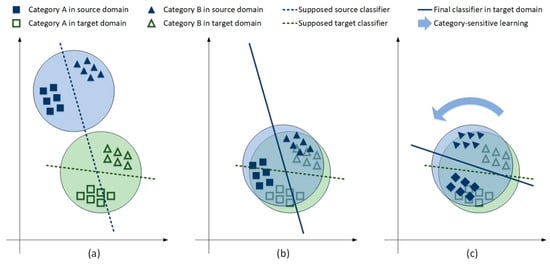
Figure 1.
Illustration of category-sensitive domain adaptation. The blue and green circles denote the marginal distributions of source and target samples, respectively. (a) Original sample distributions and two supposed classifiers. (b) Sample distributions and the final classifier by conventional global domain adaptation. (c) Sample distributions and the final classifier by our proposed category-sensitive domain adaptation (CsDA).
Motivated by the above observation, we propose a hybrid framework to simulate the process of our proposed CsDA, which consists of one encoder , one translator , and two decoders, and . The encoder aims to extract features separately from the source and target images, then the translator aims to translate the source features to the target domain while keeping the target features in the target domain. Finally, the decoders aim to classify the translated and target features produced by the translator, achieving land cover mapping simultaneously for the source and target images. To enable effective learning of this framework, we introduce three discriminators as adversaries. Two of them are global domain discriminators and , which both mainly aim to judge whether the translated and target features are distributed in the same domain, while the remaining one is a category-level discriminator , that mainly aims to judge whether the category distributions in the source and target predictions are aligned.
3.2. Framework Architecture
Our proposed CsDA is driven by a hybrid framework that is specifically designed as shown in Figure 2. The framework contains three main parts, namely, feature extraction, feature translation and feature classification respectively. And there is one encoder, one translator, and two different decoders. These four neural networks make up two primary modules: GcGAN and CtALN. As the inputs of the framework, a couple of source and target images are forwarded to the same encoder and translator respectively, being processed as the translated and target features. Thereafter, these two features are simultaneously forwarded to the two decoders, and source and target predictions will serve as the final outputs. The detailed mechanisms of our GcGAN and CtALN modules are introduced in the following subsections.
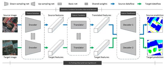
Figure 2.
Framework of our proposed category-sensitive domain adaptation for land cover mapping using very-high-resolution (VHR) optical aerial images.
3.2.1. Geometry-Consistent Generative Adversarial Network
The primary goal of the GcGAN module is to reduce the domain discrepancies between labeled and unlabeled images and to retain the intrinsic information. This module is achieved by a translator and two global domain discriminators, as illustrated in Figure 3.
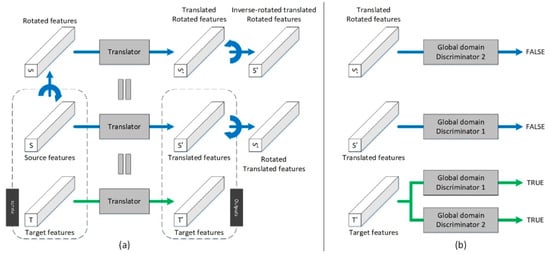
Figure 3.
Module of the geometry-consistent generative adversarial network: (a) Feature translation, (b) global domain discrimination. The blue and green arrows indicate the data flows of the source and target features, respectively. The curve arrows represent geometric rotation operations.
Given a couple of source feature maps and target feature maps as the inputs, the rotated feature maps are defined as , where is a geometric rotation function for features that satisfies . In this way, the translated rotated, translated and target feature maps can be defined as , and . To enable effective learning of the translator, two discriminators are introduced to judge whether the translated rotated and translated feature maps belong to the target domain. As the adversaries of the translator, these two discriminators try to identify the target features as real features, while identifying the translated rotated and translated features as fake features, as expressed in Equations (3) and (4):
where, and are matrices with Boolean values of 1 and 0 respectively, which denote real and fake images pixels identified by the two discriminators. In addition, the rotation-invariant constraints can be formulated shown in as Equations (5) and (6), and the identity constraint in the target domain can be formulated as shown in Equation (7):
In this module, when training, the two global domain discriminators and the rotation-invariant constraints will simultaneously facilitate updating of the translator until it can correctly translate the source features into the target domain. When testing, however, only the translator is utilized to retain the target features in the target domain.
3.2.2. Co-Training Adversarial Learning Network
The primary goal of the CtALN module is to distill knowledge from the source domain and to transfer it to the target domain, by conducting a supervised and an unsupervised semantic labeling simultaneously on the labeled and unlabeled datasets. This module is achieved by an encoder, two decoders, and a category-level discriminator, as illustrated in Figure 4.
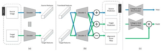
Figure 4.
Module of the co-training adversarial learning network: (a) Feature extraction, (b) feature classification, (c) category-level discrimination. The blue and green arrows indicate the data flows of the source and target images, respectively. represents element-wise summation, represents element-wise distance, and represents element-wise multiplication.
Taking a couple of source image and target image as the inputs of the feature extraction part, the source and target feature maps are defined as and , which are the inputs of the translator in the GcGAN module. Thereafter, taking the outputs of the GcGAN as the inputs of the feature classification part, the two decoders produce a source prediction map, a target prediction map and an alignment score map, which can be defined as shown in Equations (8)–(10):
where, is a distance metric to measure the element-wise discrepancy between two prediction maps, and it is chosen here to be the cosine distance. Specific to the pixel level, the alignment score map is defined as shown in Equation (11):
where, is the alignment score of the pixel located at , while and are two one-dimensional vectors located at . If the angle between these two vectors is close to 0, the pixel score will be close to 0, which means that the two decoders will make similar predictions for this pixel. Meanwhile, if the angle is close to , the pixel score will be close to 1, which means that the two decoders will make different predictions for this pixel. To enable effective learning of these two decoders, a discriminator is introduced to explore the category-level alignment degree between the source and target prediction maps. As the adversary of the two decoders, the discriminator tries to identify source predictions as real predictions, and unaligned parts of the target predictions as fake predictions, as expressed in Equation (12):
where, represents element-wise multiplication. In addition, the co-training constraint between the weights of the two decoders is formulated as shown in Equation (13), and with the reference land cover maps in the source domain, the supervised labeling constraint can be formulated as shown in Equation (14):
In this module, when training, the category-level discriminator and supervised constraint will simultaneously facilitate updating of all the networks until they can make correct predictions for the source images, while making similar predictions for the target images. When testing, however, only the encoder and two decoders are utilized to extract and classify features and then achieve land cover mapping in the target domain.
3.3. Loss Function
We propose a novel loss function comprised of six types of terms: (1) global domain adversarial loss to match the marginal distributions of the source and target features, (2) rotation-invariance loss to represent the geometry-consistency of the source features with and without rotation, (3) identity loss to encourage the translator to be the identity mapping for all the features in the target domain, (4) category-level adversarial loss to match the category-level distributions of the source and target features, (5) co-training loss to represent the divergence of the weights of the two diverse decoders and (6) labeling loss to evaluate whether all the networks are trained well for supervised land cover mapping on labeled images.
3.3.1. Global Domain Adversarial Loss
As the key loss of the GcGAN, global domain adversarial loss is a type of basic adversarial loss proposed by Goodfellow et al. [37]. This type of loss increases the ability of the generator to fool the discriminator, hindering it from distinguishing translated features from target features in the same domain. In our GcGAN module, here we apply two adversarial losses, for the translated and translated rotated features, as expressed in Equations (15) and (16), respectively:
where, tries to translate the source and rotated features to the target domain, making them similar to the target features, while and try to separate them, as shown in Equations (3) and (4). Therefore, the translator aims to minimize these losses against the discriminators that aim to maximize them, as in and .
3.3.2. Rotation-Invariance Loss
Rotation-invariance loss is a special type of reconstruction loss that relies on geometric rotation function, which was first proposed by Benaim et al. [40]. Specifically, for the rotation invariance of land cover objects in aerial images, this loss is set to enforce two couples of translated features to be similar at the pixel level. Concretized from Equations (5) and (6), the rotation-invariance loss can be expressed as shown in Equation (17):
where, is the L1 distance loss. Minimizing this loss makes our translator sensitive to land cover categories, improving the generalization ability of our framework.
3.3.3. Identity Loss
As a result of the powerful expression capabilities of deep neural networks, our solution for the translation from the source domain to the target domain is generally stochastic and not unique. To stabilize the translator, here we apply identity loss to ensure that the translator would keep the target features as invariant. Since its introduction by Taigman et al. [48], this type of loss has been widely utilized in unsupervised domain adaptation, such as DistanceGAN [40] and CycleGAN [18]. Concretized from Equation (7), identity loss can be expressed as shown in Equation (18):
where, is the L1 distance loss. Minimizing this loss decreases the randomness of our translator, providing a positive direction for the convergence procedure.
3.3.4. Category-Level Adversarial Loss
As the key loss of the CtALN, category-level adversarial loss is a type of basic adversarial loss, which is similar to the global domain adversarial loss described in Section 3.3.1. Derived from the self-adaptive adversarial loss introduced by Luo et al. [17], category-level adversarial loss aims to increase the ability of the generator to fool the discriminator, hindering it from distinguishing the unaligned parts of the target prediction from the source prediction, as expressed in Equation (19):
where, and denote and respectively. To simplify the expression of this loss, we use to represent the entire process of the framework, which satisfies . is the adaptive weight for the element-wise discrepancy between two predictions and is a small bias used to stabilize the training process. In this loss function, tries to produce correct predictions for target images without reference, while tries to separate them based on source predictions, as shown in Equation (12). Therefore, the generator aims to minimize this loss against the discriminator that aims to maximize it, as in .
3.3.5. Co-Training Loss
As first proposed by Zhou et al. [49], co-training loss is a constraint rather than a specific loss function. To provide two diverse perspectives for one semantic labeling task, the two decoders are suggested to have entirely diverse parameters. Based on this mechanism, we apply co-training loss here to enforce the divergence of the weights of all the convolutional layers in our two decoders by minimizing their cosine similarity. Concretized from Equation (13), the co-training loss can be expressed as shown in Equation (20):
where, denotes the operation used to collect all the weights of a network, then reshape and concatenate them into a one-dimensional vector. means the norm of a vector. Minimizing this loss makes our two decoders orthogonal vectorially, leading to more precise predictions for target images.
3.3.6. Labeling Loss
Labeling loss is an essential type of multi-class cross entropy loss that is often used in supervised semantic labeling tasks with FCN [9]. With source images and their reference land cover maps, we employ a LogSoftmax function as our labeling loss here to make the source predictions be near their reference labels at the pixel level. Concretized from Equation (14), the labeling loss can be expressed as shown in Equation (21):
where, means the prediction probability of category of the pixel located at , while means the reference probability of category of the pixel located at , where if this pixel belongs to category , , otherwise . Minimizing this loss makes our framework achieve supervised land cover mapping on source images.
In general, the full objective of our GcGAN module is an integration of the two global domain adversarial losses, the rotation-invariance loss and the identity loss, as formulated in Equation (22). Meanwhile, the full objective of our CtALN module is an integration of the category-level adversarial loss, the co-training loss and the labeling loss, as formulated in Equation (23):
where, denotes the relative importance for each of these six loss functions. Therefore, the overall objective of our framework can be formulated as shown in Equation (24):
Therefore, the main solutions for this overall objective can be expressed as shown in Equations (25) and (26):
Guided by certain reference land cover maps for source aerial images, we train all the networks on the same timeline. When testing, however, only the trained encoder, translator, and decoders are used for land cover mapping on unlabeled aerial images in the target domain.
3.4. Implementation
3.4.1. Network Architecture
Our proposed CsDA is driven by seven neural networks, which are one encoder, one translator, two decoders, two global domain discriminators and, one category-level discriminator respectively. The architectures of them are illustrated in Figure 5. Taking DeepLab [12] with ResNet 101 [50] as the backbone, the encoder consists of a convolutional block, a max-pooling layer, and multiple residual bottlenecks. This network conducts eightfold down-sampling on the input image patches, producing feature maps with dimensions of . The translator, derived from the generator in CycleGAN [18], is composed of six residual blocks without down- or up-sampling operation, and the decoders are both composed of three up-sampling convolutional blocks and an atrous spatial pyramid pooling (ASPP) block, followed by a LogSoftMax layer. For our three discriminators, we adopt a Markovian discrimination strategy [51] to model only the high-frequency structures of features or images, since the couple of input features or images of these discriminators are unpaired. Therefore, similar to the discriminator in pixel-to-pixel GAN [39], our three discriminators are all PatchGANs, which conduct eightfold down-sampling on the input features or images. In addition, we suggest utilizing the pre-trained model on ImageNet [52] as the backbone of the encoder. For the other six networks, all the weights and biases of their layers are initialized using the strategy of Xavier [53].
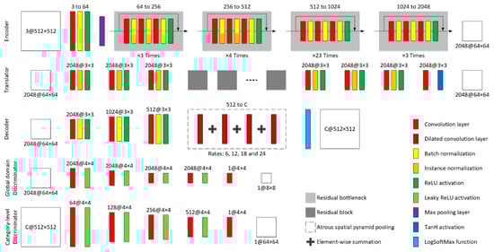
Figure 5.
Network architectures of the encoder, translator, decoder, global domain discriminator and category-level discriminator.
3.4.2. Training Detail
For all the experiments, our primary goal is to obtain well-trained models through the training process that minimizes the overall objective . In our research, according to the implementation in GcGAN [41], we set , and to 0.001, 0.02 and 0.01, respectively, in Equation (22). On the other hand, according to the implementation in CLAN [27], we set , and to 0.001, 0.01 and 1 respectively, in Equation (23), and set and to 10 and 0.4 respectively, in Equation (19). To stabilize the training process, we choose the least-squares loss specifically for and , instead of the negative log likelihood loss in traditional GANs [37,38].
Given the complexity of the hybrid framework, we utilize a hierarchical learning strategy in the optimization procedure. For the first one fifth of the epochs, we train the GcGAN module using only the objective . During this process, only the translator is being updated until it can translate the source features to the target domain effectively. Thereafter, for the last four fifths of the epochs, we train both the CtALN and GcGAN modules alternately with the objectives and . For the backward propagation in one epoch, we firstly update the encoder, the translator, and the two decoders once, and then update only the translator a second time. The overview of the training process for our hybrid framework is presented in Table 2.
Table 2.
Overview of the training process for our hybrid framework.
4. Experiments
4.1. Datasets Description
Vaihingen dataset [54]: This benchmark dataset consists of 33 aerial images collected over a 1.38 square kilometer area of the city of Vaihingen with a spatial resolution of 0.09 m/pixel. On average, these aerial images all have dimensions of approximately , and each of them has three bands corresponding to the near infrared (NIR), red (R) and green (G) bands delivered by the camera. Notably, only 16 of them are manually labeled with land cover maps, where the pixels are classified into six land cover categories, which are impervious surfaces (Imp. surf.), buildings (Build.), low vegetation (Low veg.), trees (Tree), cars (Car), and clutter/background (Clu./Back.), respectively.
Potsdam dataset [55]: This benchmark dataset consists of 38 aerial images collected over a 3.42 square kilometers area of the city of Potsdam with a spatial resolution of 0.05 m/pixel. These aerial images all have dimensions of , and each of them has four bands corresponding to the infrared (IR), red (R), green (G) and blue (B) bands. Only 24 of them are manually labeled with land cover maps, according to the same classification rules as for the Vaihingen dataset.
For these two datasets, certain basic information including the spatial resolution, mean value of each band, number of labeled/unlabeled images, and proportions of different categories, is computed and summarized in Table 3. It is notable that the different land cover categories are proportionally unbalanced, for example, cars and clutter/background are much less represented than others.
Table 3.
Basic statistics for Vaihingen and Potsdam datasets.
4.2. Methods Comparison
In this research, the performance of our proposed CsDA is compared with those of several state-of-the-art methods. As the pioneer work applying adversarial learning for unsupervised domain adaptation, CycleGAN [18] is set to be the baseline method in our comparison. As the first work applying domain adaptation for semantic segmentation, FCNwild [36] is the representative of pixel-level methods. CyCADA [23] and BDL [24] are the representatives of methods based on pixel- and feature-constraints, while CBST [26] and CLAN [27] are the representatives of methods considering category-level constraints. In addition, Benjdira et al. [14] recently cascaded a CycleGAN and a semantic segmentation model and proposed a stepwise method of achieving unsupervised domain adaptation for semantic segmentation of aerial images. As the latest land cover mapping approach, it is utilized in our comparison as well. For all the competitors, we use a same pre-trained DeepLab model with ResNet 101 as their semantic labeling models, and all the experiments are performed for the same tasks on the same datasets.
4.3. Evaluation Metrics
To prove the validity and effectiveness of the cross-domain land cover mapping methods, the following four indices are used to evaluate the accuracy of the experimental results.
Overall Accuracy (OA): The overall accuracy is generally used to assess the total capability of land cover mapping models, as expressed in Equation (27):
where, , , , and are the numbers of true positive, true negative, false positive, and false negative pixels respectively, and indicates that the index refers to the th category of ground objects.
Mean F1 Score (mF1): This statistical magnitude is the harmonic average of the precision and recall rates. It is generally used to evaluate neural network models, as expressed in Equation (28):
Intersection over Union (IoU) and Mean IoU (mIoU): These two indices are standard measures of classification-based methods. IoU calculates the ratio between the pixel numbers in the intersection and union of the prediction and reference for each category, as expressed in Equation (29):
Therefore, mIoU can be calculated as expressed in Equation (30):
It is notable that OA and mF1 mainly focus on the overall pixel accuracy, while IoU and mIoU mainly concentrate on the category-level pixel accuracy. For these four indices, large values suggest better results.
4.4. Experimental Setup
To verify the accuracy and efficiency of this method, we conduct two experiments between the aforementioned two benchmark datasets. For the Vaihingen dataset, we use the NIR, R and G bands as the pseudo RGB aerial images, while for the Potsdam dataset, we use the R, G and B bands as the true RGB aerial images. Before the experiments, it is essential to conduct certain pre-processing on these two datasets as follows:
- Unlike objects in common natural images, certain ground objects in aerial images have constant scale ranges [56]. Therefore, we make the two datasets consistent in scale, by resampling the Potsdam dataset to obtain a spatial resolution similar to that of the Vaihingen dataset.
- To accelerate the convergence of the weight and bias parameters in all the models, we perform mean-subtraction on all the aerial images. The mean values of each band in the two datasets are listed in Table 3.
In the experiments, if the Vaihingen dataset is set as the source data, we take the 16 Vaihingen labeled aerial images with their land cover maps and the 14 Potsdam unlabeled aerial images as the training data, while utilizing the 24 Potsdam labeled aerial images and their references for testing and assessment. On the contrary, if the Potsdam dataset is set as the source data, the 24 Potsdam labeled aerial images with their land cover maps and the 17 Vaihingen unlabeled aerial images are taken as the training data, while the 16 Vaihingen labeled aerial images and their references are utilized for testing and assessment. In addition, all the data involved in the experiments are small image patches with dimensions of , which are randomly cut from the two datasets.
For the optimization procedure, we set 200 epochs to achieve overall convergence, and each epoch involves 960 iterations. For the encoder, translator and two decoders, we used stochastic gradient decent (SGD) with a momentum [57] of 0.9 as the optimizer, where the initial learning rate is set to and progressively decayed to 0 by a poly learning rate policy. Meanwhile, for all the discriminators, we use Adaptive Moment Estimation (Adam) [58] as the optimizer, where the initial learning rate is set to and linearly decayed to 0. The decay rates for the moment estimates are 0.9 and 0.999 respectively, and the epsilon is .
In the present research, our proposed CsDA is implemented in a PyTorch environment, which offers an effective programming interface written in Python. The experiments are performed on a computer with Intel Core i7, 32GB RAM, and NVIDIA GTX 1080 GPU. When training, the times for the partial epoch and entire epoch are 335 and 1210 seconds, respectively. With 200 epochs, the entire time for the training process of one experiment is approximately 58 hours. On the other hand, when testing, the time for one target aerial image patch with dimensions of is just 0.19 second.
4.5. Result Presentation
For the two experiments: from Vaihingen to Potsdam and from Potsdam to Vaihingen, the land cover mapping results obtained using our proposed CsDA and all the competitors are presented in Figure 6 and Figure 7, where the white, blue, cyan, green, yellow, and red regions respectively indicate the categories of impervious surfaces, buildings, low vegetation, trees, cars, and clutter/background. As can be seen, the testing results of the Vaihingen dataset are visually better than those of the Potsdam dataset, because, as guidance for each other, the Potsdam land cover maps are annotated more elaborately and precisely than the Vaihingen land cover maps.
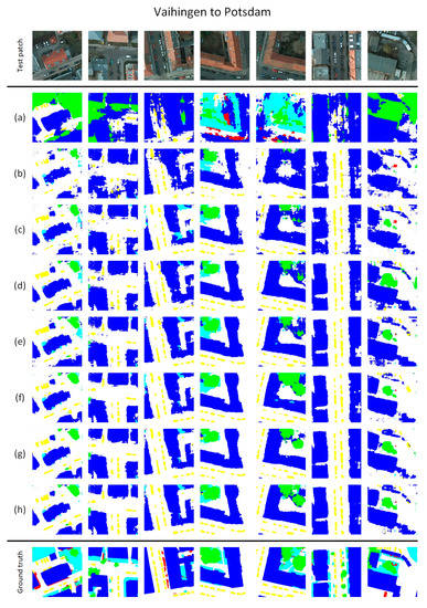
Figure 6.
Representative examples of land cover mapping results for the adaptation from Vaihingen to Potsdam: (a) CycleGAN, (b) FCNwild, (c) Benjdira’s, (d) CyCADA, (e) BDL, (f) CBST, (g) CLAN, (h) our CsDA.
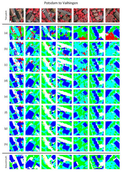
Figure 7.
Representative examples of land cover mapping results for the adaptation from Potsdam to Vaihingen: (a) CycleGAN, (b) FCNwild, (c) Benjdira’s, (d) CyCADA, (e) BDL, (f) CBST, (g) CLAN, (h) our CsDA.
Since CycleGAN is merely an unsupervised domain adaptation method that is agnostic to any particular task, its testing results are full of errors and uncertainties, as shown in Figure 6a and Figure 7a. As the representatives of pixel-level methods, FCNwild and Benjdira’s methods give approximate positions for the land cover categories but ambiguous outlines. Due to the weak constraints at the pixel level, their testing results remain unsatisfactory for real applications, as shown in Figure 6b,c, or Figure 7b,c. With the addition of feature-level constraints, CyCADA and BDL yield better results than the pixel-level methods. Especially in terms of ground object distributions, feature-level constraints can facilitate the models encouraging individuals to be distinctly isolated from one another. However, certain boundaries between different categories of ground objects remain rough, while certain predictions of large-scale ground objects involve many holes, as shown in Figure 6d,e, or Figure 7d,e. By considering category-level constraints, CBST and CLAN are able to achieve more precise and clearer predictions, which are largely free from noise, as shown in Figure 6f,g, or Figure 7f,g. These findings confirm that, for cross-domain land cover mapping, category-level constraints provide superior guidance compared to the other constraints. As shown in Figure 6h and Figure 7h, our proposed CsDA, which considers multiple constraints and geometry consistency, achieved the best testing results, where the contours of the predicted ground objects are more accurate and smoother than those obtained using CBST and CLAN.
With the testing results obtained using our proposed CsDA and other comparative methods, the evaluation metrics OA, mF1, IoU and mIoU, and the processing rate for these two cross-domain land cover mapping experiments are computed and summarized in Table 4 and Table 5. Compared with other state-of-the-art methods, although our proposed CsDA has a slower processing rate of 0.19 second per image patch, it achieves the highest OA, mF1, and mIoU values of 60.4%, 52.8% and 42.3% in the experiment from Vaihingen to Potsdam and 65.3%, 54.5% and 44.9% in the experiment from Potsdam to Vaihingen, respectively.
Table 4.
Comparison results based on the domain adaptation from Vaihingen to Potsdam. The best values are in bold.
Table 5.
Comparison results based on the domain adaptation from Potsdam to Vaihingen. The best values are in bold.
5. Discussion
For cross-domain land cover mapping approaches based on deep learning, the performance is mainly dominated by three decisive factors, which are the framework architecture, loss function, and optimization strategy. In this section, the discussions of our designs of these three factors verify the robustness and superiority of our method.
5.1. Design of Framework Architectures
Regarding unsupervised domain adaptation for semantic labeling, current researchers generally focus on training multi-module joint frameworks sequentially. In this manner, source images are first utilized to learn the domain adaptation model, then the translated and target images are utilized to learn the semantic labeling model. Taking our two modules as the backbone, the framework can be designed as depicted in Figure 8. We conducted several comparative experiments using these two types of frameworks for the same tasks, and the testing results are presented in Figure 9.
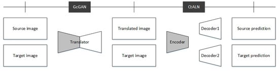
Figure 8.
Framework of the cascaded architecture based on our GcGAN and CtALN modules.
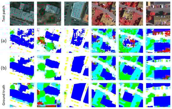
Figure 9.
Representative examples of land cover mapping results driven by two different frameworks: (a) Cascaded architecture, (b) embedded architecture. The left three test patches are from the Potsdam dataset while the right three test patches are from the Vaihingen dataset.
As can be seen, compared with the embedded framework of our proposed CsDA, the cascaded framework is more concise and easier for training, but its performance is poor. Especially for certain complex large-scale ground objects, this framework cannot yield complete and clear predictions. The primary problems can be summarized as follows:
- Since the inputs and outputs of the GcGAN are both images, the cascaded framework does not consider the feature-level alignment between the labeled and unlabeled image patches during the domain adaptation process.
- The cascaded framework uses high-frequency features, which are extracted from the translated images, to train the CtALN. The features may involve numerous errors and uncertainties, since they are not directly extracted from the source images.
- When training, the cascaded framework conducts two down-sampling operations, referring to the two gray trapezoidal blocks in Figure 8, which may lose significant detailed information. In comparison, our embedded framework conducts only one down-sampling operation.
5.2. Design of Loss Functions
As the representative of training goal, the loss functions determine the qualities of the trained models. To validate the effectiveness and uniqueness of our loss functions, we conduct two ablation studies separately for the two experiments. Then the testing OAs and mIoUs driven by five diverse combinations of loss functions are computed and summarized in Table 6. In the following, we will provide detailed interpretations of the effects of each loss function.
Table 6.
Ablation studies of the overall objective for our two experiments.
It is noteworthy that the first combination represents a framework integrating a GcGAN and a simple semantic labeling model, while the second one represents a framework integrating a simple domain adaptation model and a CtALN.
By comparing the first, third, and last rows in Table 6, it is evident that the addition of category-level adversarial loss can slightly improve the performance and that the addition of co-training loss can significantly improve the performance. The distinct increases in OAs and mIoUs indicate that, despite the absence of reference labels in the target domain, the two orthogonal decoders also can facilitate pursuit of the correct predictions. Due to the powerful unsupervised classification ability, this multi-view learning strategy is specifically applicable to cross-domain land cover mapping.
By comparing the second, fourth, and last rows in Table 6, it is evident that the additions of rotation-invariant and identity loss both can effectively improve the performance. In practice, these two losses are specifically designed for remote sensing types of data, since almost all ground objects in aerial images are of geometry-consistency. Notably, although these two constraints facilitate the training of better land cover mapping models, they seem to be beneficial merely for the recognition of large-scale ground objects such as buildings and trees, while for the recognition of small ground objects such as cars and clutter/background, they may have certain negative impacts, as illustrated in Table 4 and Table 5.
5.3. Design of Optimization Strategies
In the training process, the multi-module joint framework involves a major limitation, which was noted in Reference [59]. Taking our hybrid framework as an example, in the early period of training, the encoder and decoders updates are useless, since the GcGAN cannot achieve feature translation from the source domain to the target domain at that time. Furthermore, simultaneously training the GcGAN and CtALN modules will give wrong guidance to the encoder and decoders, leading to certain irregular oscillations on the convergence curves. To address this issue, we utilized a hierarchical learning strategy in the optimization procedure, as introduced in Table 2 in Section 3.4.2. Based on our proposed CsDA, we conduct joint learning and hierarchical learning separately in two experiments, and all the convergence curves are compared in Figure 10. As introduced in Section 3.4.2, during the hierarchical learning process, the curve of the GcGAN objective starts at the beginning, while the curve of the CtALN objective appears at the 41st epoch.
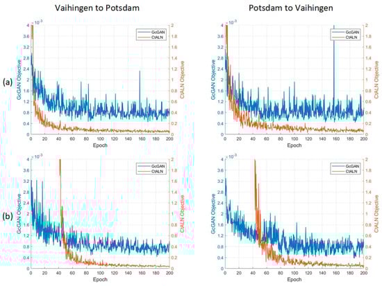
Figure 10.
Convergence curves for our two experiments with two different optimization strategies: (a) Joint learning and (b) hierarchical learning.
It is noteworthy that, although the joint learning strategy encourages the losses of the GcGAN and CtALN to decline simultaneously, incorrect guidance from the GcGAN in the early stage makes the training process unstable, leading to certain huge oscillations even in the late stage, as shown in Figure 10a. In comparison, the hierarchical learning strategy can facilitate stabilization of the training process, especially in the late stage, and the convergence curves of the CtALN are smoother than that by the joint learning strategy, as illustrated in Figure 10b. As a result, the experimental performance with the hierarchical learning strategy is slightly better than that with the joint learning strategy.
In addition, the entire times for training 200 epochs with these two strategies are approximately 67.2 and 58 hours, respectively. Compared with the joint learning strategy, the hierarchical learning strategy has saved nearly 9.2 hours.
6. Conclusions
In this research, we embedded a GcGAN into a CtALN, then developed a CsDA for land cover mapping using VHR optical aerial images. With the proposed GcGAN, we successfully eliminated the domain discrepancies between labeled and unlabeled images by translating the features of the labeled images into the target domain. The proposed CtALN successfully distilled knowledge from the source images and corresponding reference labels, then achieved land cover mapping for the target images without reference labels. Massive experiments between the Vaihingen and Potsdam datasets confirmed the robustness and superiority of our proposed CsDA, which yielded competitive land cover mapping performance compared with other state-of-the-art domain adaptation methods.
Nevertheless, our method involves a major limitation. With only the alignment score maps for guidance in the target domain, our proposed CsDA cannot generate precise inter-class boundaries for different land cover categories. Therefore, in future studies, on the premise of ensuring land cover mapping accuracy, we plan to explore certain unsupervised contour-sensitive constraints to further improve the performance of our models.
Author Contributions
B.F. and L.P. conceived and designed the experiments; B.F. performed the experiments; R.K. and P.C. analyzed the data; R.K. contributed reagents/materials/analysis tools; B.F. wrote the paper. All authors read and approved the submitted manuscript.
Funding
This research received no external funding.
Conflicts of Interest
The authors declare no conflict of interest.
References
- Cihlar, J. Land Cover Mapping of Large Areas from Satellites: Status and Research Priorities. Int. J. Remote Sens. 2000, 21, 1093–1114. [Google Scholar] [CrossRef]
- Foody, G.M. Status of Land Cover Classification Accuracy Assessment. Remote Sens. Environ. 2002, 80, 185–201. [Google Scholar] [CrossRef]
- Congalton, R.G.; Gu, J.; Yadav, K.; Thenkabail, P.; Ozdogan, M. Global Land Cover Mapping: A Review and Uncertainty Analysis. Remote Sens. 2014, 6, 12070–12093. [Google Scholar] [CrossRef]
- Stewart, I.D.; Oke, T.R. Local Climate Zones for Urban Temperature Studies. Bull. Am. Meteorol. Soc. 2012, 93, 1879–1900. [Google Scholar] [CrossRef]
- Margono, B.A.; Potapov, P.V.; Turubanova, S.; Stolle, F.; Hansen, M.C. Primary Forest Cover Loss in Indonesia over 2000–2012. Nat. Clim. Chang. 2014, 4, 730–735. [Google Scholar] [CrossRef]
- Qi, Z.; Yeh, A.G.O.; Li, X.; Zhang, X. A Three-Component Method for Timely Detection of Land Cover Changes using Polarimetric SAR Images. ISPRS J. Photogramm. Remote Sens. 2015, 107, 3–21. [Google Scholar] [CrossRef]
- Garcia-Garcia, A.; Orts-Escolano, S.; Oprea, S.O.; Villena-Martinez, V.; Garcia-Rodriguez, J. A Review on Deep Learning Techniques Applied to Semantic Segmentation. arXiv 2017, arXiv:1704.06857. [Google Scholar]
- Lateef, F.; Ruichek, Y. Survey on Semantic Segmentation using Deep Learning Techniques. Neurocomputing 2019, 338, 321–348. [Google Scholar] [CrossRef]
- Long, J.; Shelhamer, E.; Darrell, T. Fully Convolutional Network for Semantic Segmentation. In Proceedings of the IEEE Conference on Computer Vision and Pattern Recognition, Boston, MA, USA, 7–12 June 2015; pp. 3431–3440. [Google Scholar]
- Ronneberger, O.; Fischer, P.; Brox, T. U-Net: Convolutional Networks for Biomedical Image Segmentation. In Proceedings of the International Conference on Medical Image Computing and Computer-Assisted Intervention, Munich, Germany, 5–9 October 2015; Springer: Cham, Switzerland, 2015; pp. 234–241. [Google Scholar]
- Badrinarayanan, V.; Kendall, A.; Cipolla, R. SegNet: A Deep Convolutional Encoder-Decoder Architecture for Image Segmentation. IEEE Trans. Pattern Anal. Mach. Intell. 2017, 39, 2481–2495. [Google Scholar] [CrossRef]
- Chen, L.C.; Papandreou, G.; Kokkinos, I.; Murphy, K.; Yuille, A.L. DeepLab: Semantic Image Segmentation with Deep Convolutional Nets, Atrous Convolution, and Fully Connected CRFs. IEEE Trans. Pattern Anal. Mach. Intell. 2018, 40, 834–848. [Google Scholar] [CrossRef]
- Pan, S.J.; Yang, Q. A Survey on Transfer Learning. IEEE Trans. Knowl. Data Eng. 2010, 22, 1345–1359. [Google Scholar] [CrossRef]
- Benjdira, B.; Bazi, Y.; Koubaa, A.; Ouni, K. Unsupervised Domain Adaptation using Generative Adversarial Networks for Semantic Segmentation of Aerial Images. Remote Sens. 2019, 11, 1369. [Google Scholar] [CrossRef]
- Ben-David, S.; Blitzer, J.; Crammer, K.; Kulesza, A.; Pereira, F.; Vaughan, J.W. A Theory of learning from different domains. Mach. Learn. 2010, 79, 151–175. [Google Scholar] [CrossRef]
- Wang, M.; Deng, W. Deep Visual Domain Adaptation: A Survey. Neurocomputing 2018, 312, 135–153. [Google Scholar] [CrossRef]
- Tzeng, E.; Hoffman, J.; Saenko, K.; Darrell, T. Adversarial Discriminative Domain Adaptation. In Proceedings of the Computer Vision and Pattern Recognition (CVPR), Honolulu, HI, USA, 21–26 July 2017; Volume 1, p. 4. [Google Scholar]
- Zhu, J.; Park, T.; Isola, P.; Efros, A. Unpaired Image-to-Image Translation Using Cycle-Consistent Adversarial Networks. In Proceedings of the IEEE International Conference on Computer Vision (ICCV), Venice, Italy, 22–29 October 2017; pp. 2223–2232. [Google Scholar]
- Sankaranarayanan, S.; Balaji, Y.; Jain, A.; Lim, S.N.; Chellappa, R. Unsupervsed Domain Adaptation for Semantic Segmentation with GANs. arXiv 2017, arXiv:1711.06969. [Google Scholar]
- Bengio, Y.; Louradour, J.; Collobert, R.; Weston, J. Curriculum learning. In Proceedings of the 26th Annual International Conference on Machine Learning, Montreal, QC, Canada, 14–18 June 2009; Volume 2, pp. 41–48. [Google Scholar]
- Zhang, Y.; David, P.; Gong, B. Curriculum Domain Adaptation for Semantic Segmentation of Urban Scenes. In Proceedings of the IEEE International Conference on Computer Vision (ICCV), Venice, Italy, 22–29 October 2017. [Google Scholar]
- Tsai, T.-H.; Hung, W.-C.; Schulter, S.; Sohn, K.; Yang, M.-H.; Chandraker, M. Learning to Adapt Structured Output Space for Semantic Segmentation. arXiv 2018, arXiv:1802.10349. [Google Scholar]
- Hoffman, J.; Tzeng, E.; Park, T.; Zhu, J.; Isola, P.; Saenko, K.; Efros, A.A.; Darrell, T. CyCADA: Cycle-Consistent Adversarial Domain Adaptation. arXiv 2017, arXiv:1711.03213. [Google Scholar]
- Li, Y.; Yuan, L.; Vasconcelos, N. Bidirectional Learning for Domain Adaptation of Semantic Segmentation. arXiv 2019, arXiv:1904.10620. [Google Scholar]
- Wu, Z.; Han, X.; Lin, Y.; Uzunbas, M.G.; Goldstein, T.; Lim, S.N.; Davis, L.S. DCAN: Dual Channel-Wise Alignment Networks for Unsupervised Scene Adaptation. arXiv 2018, arXiv:1804.05827. [Google Scholar]
- Zou, Y.; Yu, Z.; Kumar, B.V.; Wang, J. Unsupervised Domain Adaptation for Semantic Segmentation via Class-Balanced Self-Training. In Proceedings of the European Conference on Computer Vision (ECCV), Munich, Germany, 8–14 September 2018; pp. 289–305. [Google Scholar]
- Luo, Y.; Zheng, L.; Guan, T.; Yu, J.; Yang, Y. Taking A Closer Look at Domain Shift: Category-Level Adversaries for Semantic Consistent Domain Adaptation. arXiv 2018, arXiv:1809.09478. [Google Scholar]
- Richter, S.R.; Vineet, V.; Roth, S.; Koltun, V. Playing for Data: Ground Truth from Computer Games. In Proceedings of the European Conference on Computer Vision (ECCV), Amsterdam, The Netherlands, 8–16 October 2016; pp. 102–118. [Google Scholar]
- Ros, G.; Sellart, L.; Materzynska, J.; Vazquez, D.; Lopez, A.M. The Synthia Dataset: A Large Collection of Synthetic Images for Semantic Segmentation of Urban Scenes. In Proceedings of the IEEE Conference on Computer Vision and Pattern Recognition (CVPR), Las Vegas, NV, USA, 27–30 June 2016; pp. 3234–3243. [Google Scholar]
- Cordts, M.; Omran, M.; Ramos, S.; Rehfeld, T.; Enzweiler, M.; Benenson, R.; Franke, U.; Roth, S.; Schiele, B. The Cityscapes Dataset for Semantic Urban Scene Understanding. In Proceedings of the IEEE Conference on Computer Vision and Pattern Recognition (CVPR), Las Vegas, NV, USA, 27–30 June 2016; pp. 3213–3223. [Google Scholar]
- Brostow, G.J.; Shotton, J.; Fauqueur, J.; Cipolla, R. Segmentation and Recognition Using Structure from Motion Point Clouds. In Proceedings of the European Conference on Computer Vision, Marseille, France, 12–18 October 2008; Volume 2, pp. 44–57. [Google Scholar]
- Saenko, K.; Kulis, B.; Fritz, M.; Darrell, T. Adapting Visual Category Models to New Domains. In Proceedings of the European Conference on Computer Vision (ECCV), Crete, Greece, 5–11 September 2010; Volume 2, pp. 213–226. [Google Scholar]
- LeCun, Y.; Bottou, L.; Bengio, Y.; Haffner, P. Gradient-Based Learning Applied to Document Recognition. Proc. IEEE 1998, 86, 2278–2324. [Google Scholar] [CrossRef]
- Friedman, J.; Hastie, T.; Tibshirani, R. The Elements of Statistical Learning; Springer Series in Statistics: New York, NY, USA, 2001. [Google Scholar]
- Netzer, Y.; Wang, T.; Coates, A.; Bissacco, A.; Wu, B.; Ng, A.Y. Reading Digits in Natural Images with Unsupervised Feature Learning. In Proceedings of the NIPS Workshop on Deep Learning and Unsupervised Feature Learning, Granada, Spain, 12–17 December 2011. [Google Scholar]
- Hoffman, J.; Wang, D.; Yu, F.; Darrell, T. FCNs in the Wild: Pixel-Level Adversarial and Constraint-Based Adaptation. arXiv 2016, arXiv:1612.02649. [Google Scholar]
- Goodfellow, I.J.; Pouget-Abadie, J.; Mirza, M.; Xu, B.; Warde-Farley, D.; Ozair, S.; Courville, A.; Bengio, Y. Generative Adversarial Nets. In Proceedings of the International Conference Neural Information Processing Systems (NIPS), Montreal, QC, Canada, 8–13 December 2014. [Google Scholar]
- Mirza, M.; Osindero, S. Conditional Generative Adversarial Nets. arXiv 2014, arXiv:1141.1784. [Google Scholar]
- Isola, P.; Zhu, J.; Zhou, T.; Efros, A.A. Image-to-Image Translation with Conditional Adversarial Networks. Proceeding of the Computer Vision and Pattern Recognition (CVPR), Honolulu, HI, USA, 21–26 July 2017; p. 632. [Google Scholar]
- Benaim, S.; Wolf, J. One-Sided Unsupervised Domain Mapping. arXiv 2017, arXiv:1706.00826v2. [Google Scholar]
- Fu, H.; Gong, M.; Wang, C.; Batmanghelich, K.; Zhang, K.; Tao, D. Geometry-Consistent Generative Adversarial Networks for One-Sided Unsupervised Domain Mapping. arXiv 2018, arXiv:1809.05852. [Google Scholar]
- Balcan, M.F.; Blum, A.; Yang, K. Co-Training and Expansion: Towards Bridging Theory and Practice. In Proceedings of the NIPS, Vancouver, BC, Canada, 13–18 December 2004. [Google Scholar]
- Saito, K.; Ushiku, Y.; Harada, T.; Saenko, K. Adversarial Dropout Regularization. arXiv 2017, arXiv:1711.01575. [Google Scholar]
- Saito, K.; Watanabe, Y.; Ushiku, Y.; Harada, T. Maximum Classifier Discrepancy for Unsupervised Domain Adaptation. arXiv 2017, arXiv:1712.02560. [Google Scholar]
- Zhang, J.; Liang, C.; Kuo, C.-C.J. A Fully Convolutional Tri-Branch Network (FCTN) for Domain Adaptation. arXiv 2017, arXiv:1711.03694. [Google Scholar]
- Chen, M.; Weinberger, K.Q.; Blitzer, J. Co-Training for Domain Adaptation. In Proceedings of the 24th International Conference on Neural Information Processing Systems, Granada, Spain, 12–15 December 2011; pp. 2456–2464. [Google Scholar]
- Saito, K.; Ushiku, Y.; Harada, T. Asymmetric Tri-Training for Unsupervised Domain Adaptation. arXiv 2017, arXiv:1702.08400. [Google Scholar]
- Taigman, Y.; Polyak, A.; Wolf, L. Unsupervised Cross-Domain Image Generation. In Proceedings of the ICLR, Toulon, France, 24–26 April 2017. [Google Scholar]
- Zhou, Z.; Li, M. Tri-Training: Exploiting Unlabeled Data Using Three Classifiers. IEEE Trans. Knowl. Data Eng. 2005, 17, 1529–1541. [Google Scholar] [CrossRef]
- He, K.; Zhang, X.; Ren, S.; Sun, J. Deep Residual Learning for Image Recognition. In Proceedings of the IEEE Conference Computer Vision and Pattern Recognition, Las Vegas, NV, USA, 27–30 June 2016; pp. 770–778. [Google Scholar]
- Li, C.; Wand, M. Precomputed Real-Time Texture Synthesis with Markovian Generative Adversarial Networks. In Proceedings of the European Conference on Computer Vision, Amsterdam, The Netherlands, 8–16 October 2016. [Google Scholar]
- Deng, J.; Dong, W.; Socher, R.; Li, L.; Li, K.; Fei-Fei, L. ImageNet: A Large-Scale Hierarchical Image Database. In Proceedings of the IEEE Conference on Computer Vision and Pattern Recognition, Miami, FL, USA, 20–25 June 2009; pp. 248–255. [Google Scholar]
- Glorot, X.; Bengio, Y. Understanding the Difficulty of Training Deep Feedforward Neural Networks. In Proceedings of the Thirteenth International Conference on Artificial Intelligence and Statistics, Sardinia, Italy, 13–15 May 2010; Volume 9, pp. 249–256. [Google Scholar]
- International Society for Photogrammetry and Remote Sensing. 2D Semantic Labeling–Vaihingen Data. Available online: http://www2.isprs.org/commissions/comm3/wg4/2d-sem-label-vaihingen.html (accessed on 11 August 2018).
- International Society for Photogrammetry and Remote Sensing. 2D Semantic Labeling Contest—Potsdam. Available online: http://www2.isprs.org/commissions/comm3/wg4/2d-sem-label-potsdam.html (accessed on 11 August 2018).
- Deng, Z.; Sun, H.; Zhou, S.; Zhao, J.; Lei, L.; Zou, H. Multi-Scale Object Detection in Remote Sensing Imagery with Convolutional Neural Networks. ISPRS J. Photogramm. Remote Sens. 2018, 145, 3–22. [Google Scholar] [CrossRef]
- Qian, N. On the Momentum Term in Gradient Decent Learning Algorithms. Neural Netw. 1999, 12, 145–151. [Google Scholar] [CrossRef]
- Kimgma, D.P.; Ba, J.L. Adam: A Method for Stochastic Optimization. In Proceedings of the International Conference on Learning Representations, San Diego, CA, USA, 7–9 May 2015; pp. 1–13. [Google Scholar]
- Fang, B.; Pan, L.; Kou, R. Dual Learning-Based Siamese Framework for Change Detection Using Bi-Temporal VHR Optical Remote Sensing Images. Remote Sens. 2019, 11, 1292. [Google Scholar] [CrossRef]


© 2019 by the authors. Licensee MDPI, Basel, Switzerland. This article is an open access article distributed under the terms and conditions of the Creative Commons Attribution (CC BY) license (http://creativecommons.org/licenses/by/4.0/).