A Method of Fast and Simultaneous Calibration of Many Mobile FMCW Radars Operating in a Network Anti-Drone System

Abstract

A market for small drones is developing very fast. They are used for leisure activities and exploited in commercial applications. However, there is a growing concern for accidental or even criminal misuses of these platforms. Dangerous incidents with drones are appearing more often, and have caused many institutions to start thinking about anti-drone solutions. There are many cases when building stationary systems seems to be aimless since the high cost does not correspond with, for example, threat frequency. In such cases, mobile drone countermeasure systems seem to perfectly meet demands. In modern mobile solutions, frequency modulated continuous wave (FMCW) radars are frequently used as detectors. Proper cooperation of many radars demands their measurements to be brought to a common coordinate system—azimuths must be measured in the same direction (preferably the north). It requires calibration, understood as determining constant corrections to measured angles. The article presents the author’s method of fast, simultaneous calibration of many mobile FMCW radars operating in a network. It was validated using 95,000 numerical tests. The results show that the proposed method significantly improves the north orientation of the radars throughout the whole range of the initial errors. Therefore, it can be successfully used in practical applications.

1. Introduction

A market of small unmanned aerial vehicles (UAVs)—commonly called drones—is developing very fast [1] and is stimulated by a very good quality to price ratio—for a relatively small amount a drone can be bought that has excellent performance regarding the possibility of flight and shooting a high-quality video from the air. Unfortunately, the drones could be used not only for commercial, research, surveillance, fun, or any other legal activities but also as a tool of crime. Sometimes intentionally, like in the case of drug smuggling across prison walls or dropping explosive materials [2]. Another time inappropriate and dangerous use of drones is caused by curiosity or lack of imagination. Camera-equipped UAVs can invade people’s privacy or cause a threat to their life. 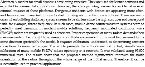For example, the report by Bard College’s Center for the Study of the Drone [3] found that 327 incidents between December 2013 and September 2015 (USA only) posed a "proximity danger" where an unmanned aircraft got within 500 feet (152.4 m) of a plane, helicopter, or other manned aircraft (involved multiengine jet aircraft). The above mentioned, as well as similar accidents, have caused many institutions to start thinking about anti-drone solutions. In the case of objects permanently threatened by drones, for example, airports or buildings crucial for national security, stationary anti-drone systems can be justified. However, there are many cases when using a permanent solution seems to be aimless due to the high cost of the system not corresponding with threat frequency, for example, mass events or meetings with very important persons (VIP). For protecting people and objects in such cases, mobile systems (on vehicle or man-carried) perfectly meet the demands. As an example of such solutions, anti-drone systems Hawk by Hertz Systems Ltd (Poland) [4] and Radar Backpack Kit by SpotterRF (USA) [5], are presented in Figure 1.

Many scientists and engineers involved in the development of anti-drone systems agree that a multi-sensor system could provide a higher probability of drone detection than a single sensor [6,7,8,9,10,11,12]. Experiments also suggest that one of the most efficient detectors of UAV is a frequency modulated continuous wave (FMCW) radar [6,7,8,9,10,11,12]. It has a big detection range, transmits low power [13], and is independent of electromagnetic signals and sounds emitted by drones (UAV operating in a fully autonomous mode and gliding can be detected, too).

Active radars do measurements in a local polar system, where distance and azimuth of the detected object are determined. Three-dimensional radars also provide information about the object elevation. It means that the accuracy of determining the drone localization in a global coordinate system depends not only on the radar performance but also on the accuracy of the radar coordinates and spatial orientation relative to the local horizon and the north. Admittedly, using precise Global Navigation Satellite System (GNSS) positioning, for example, Real Time Kinematic (RTK), can solve the problem of accurate localization. Orientation angles can also be relatively easily determined in the case of a stationary system. However, there would be some difficulties in mobile solutions, especially if the system changes location during the mission. Obviously, some sophisticated techniques, like Moving Base RTK, can provide precise orientation angles; however, using them is not always possible. They also do not ensure expected accuracy in every condition and require additional devices and often specialized knowledge. Although a magnetic compass could be a low-cost and convenient solution, it is not accurate enough if we consider that accuracy better than $1^0$ is required. Due to magnetic variation, magnetic deviation, errors connected with radar and magnetic sensor installation on a vehicle, and method of measurement, accuracy better than ${20}^0$ is difficult to achieve in a real application.

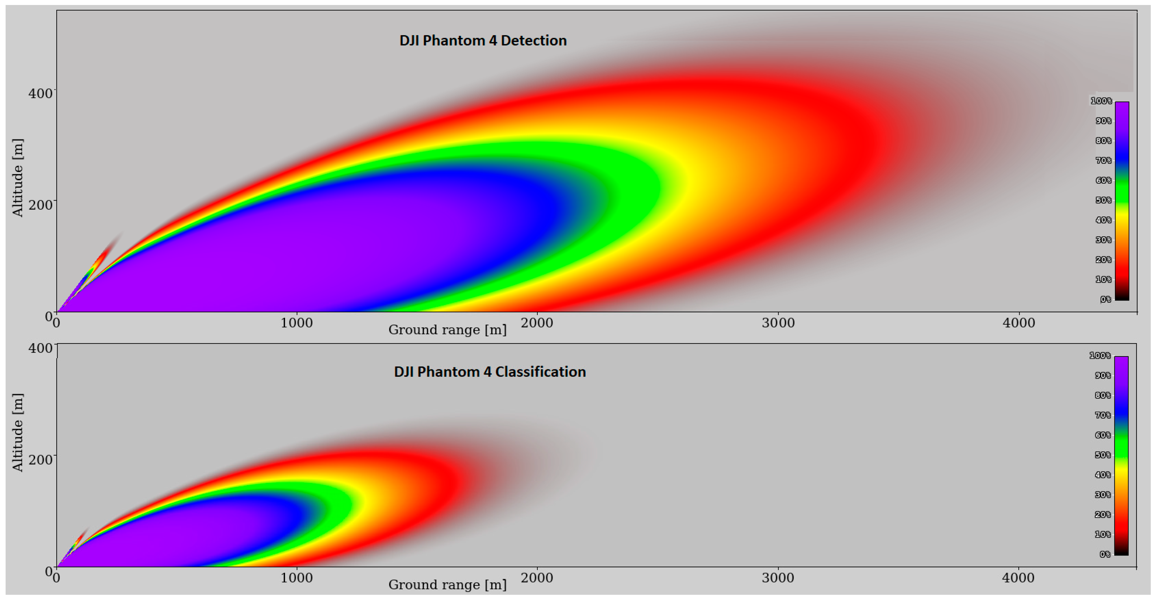
Long-range FMCW radars used in non-military anti-drone systems have detection ranges of micro-drones (DJI Phantom sizes) not exceeding 3 km, due to the small radar cross section (RCS) of such objects [14,15,16,17]. However, the classification range has a practical meaning, as anti-drone radars also detect birds and other small objects. Determining if the object is a drone allows relevant actions to be taken. The most common method of classification is the micro-Doppler signature (MDS) analysis. It allows investigating micromotions of the object detected by the radar. The contributions of the rotating turbine or propeller blades in radar backscattering in the form of micro-Doppler contents contain information that there are rotating parts on the object. On this basis, the method distinguishes a drone from a bird [18,19,20,21,22,23]. If the analysis of MDS is a classifier, the classification range is about 50% of the detection range, due to the RCS of the rotating turbine or propeller blades being smaller than the RCS of the drone body. The classification range is the range in which the classifier works accurately. Examples of detection and classification characteristics of the DJI Phantom 4 drone for one of the anti-drone radars are presented in Figure 2. It should be noted that it is currently one of the radars with the longest range of the micro-drone detection and classification available on the commercial market.

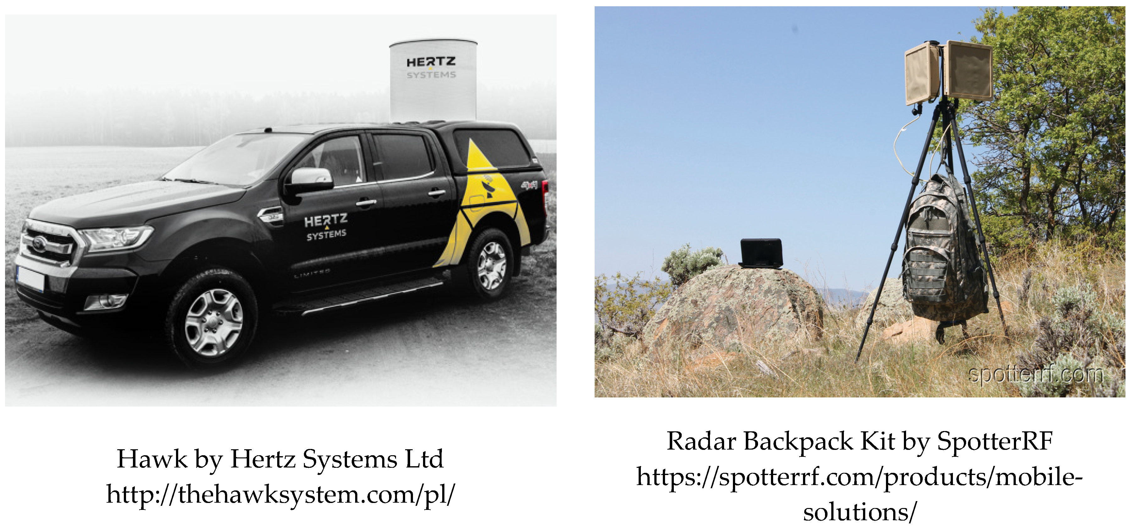
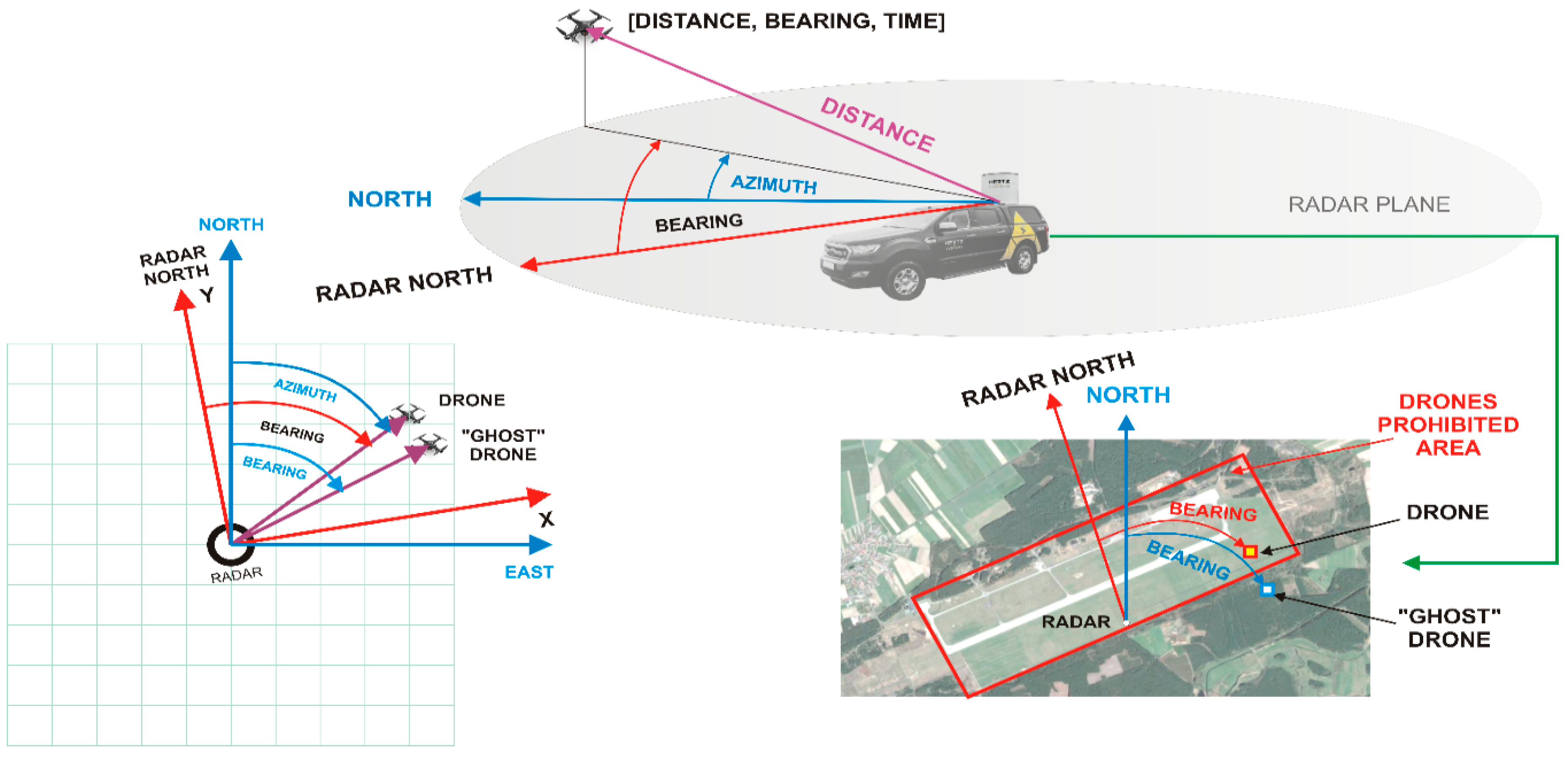
Considering the real range of non-military FMCW radars and the fact that effective protection of the area or object requires detection and classification of the drone several hundred meters before the forbidden zone, it is often necessary to use several mobile systems operating in the network. One of the key conditions for their proper cooperation is the measurement of azimuths relative to the same direction (preferably geographical north, also called the true north, or just, the north). Otherwise, errors will occur in determining the actual location of the drone. In a single-radar system, a large error in determining the coordinates of the detected object may result in incorrect classification as an object “violating” or “not violating” the forbidden area (see Figure 3) and, consequently, an inadequate response. 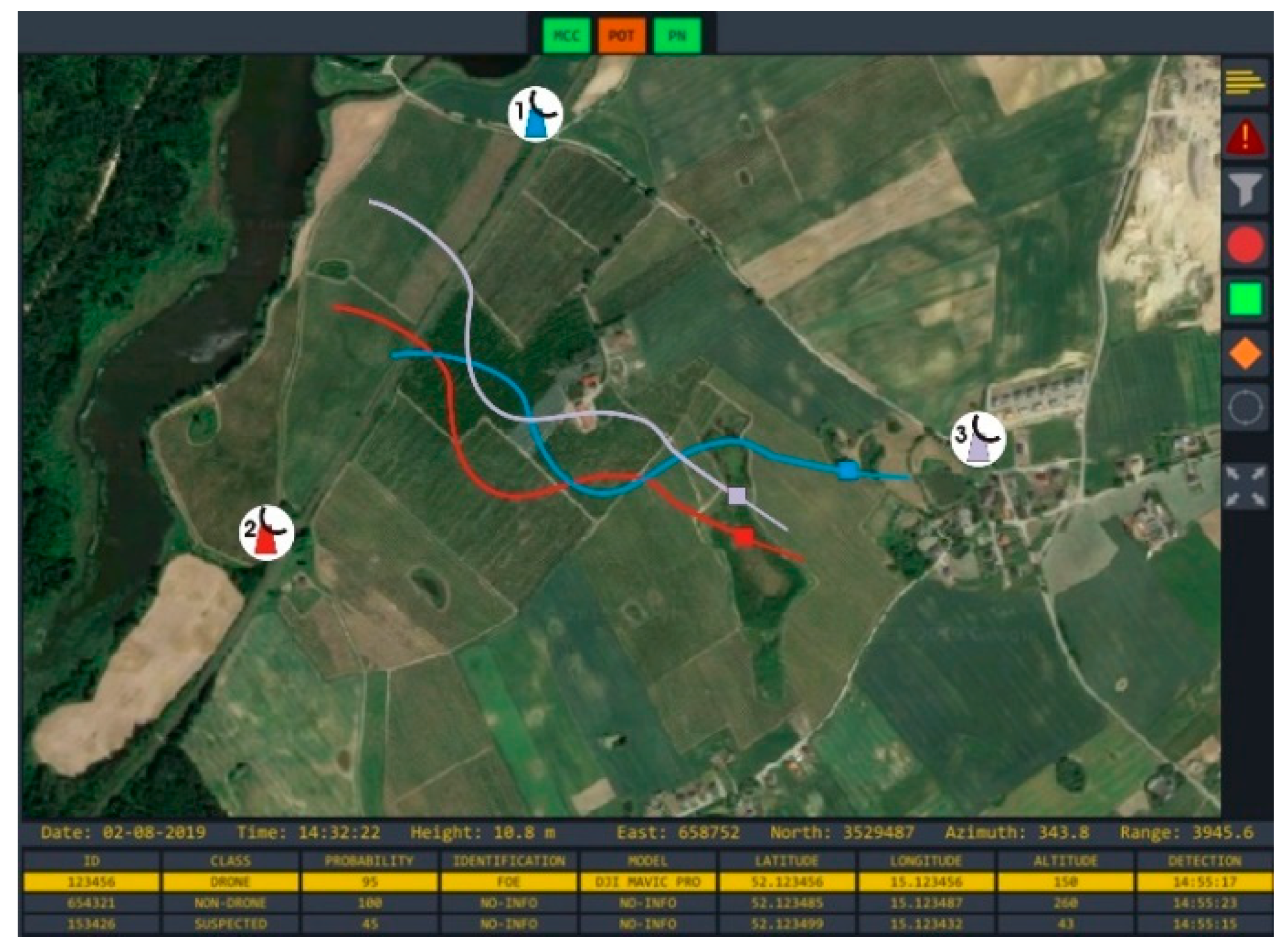In network systems, where several radars operate in the same area and their coverages partly overlap, there will be additional uncertainty concerning a location of the detected drone—each of the radars will indicate different coordinates of the same object (see Figure 4). Moreover, one will not know how many objects are really in the area. A single drone can be classified as a swarm or vice versa. All described cases are very undesirable, and their elimination is necessary to ensure the proper functioning of the anti-drone system.

Due to the fact that non-military anti-drone systems are still developing and many of them are on a low Technology Readiness Level (TRL) - similarly as some of the radar solutions in this area [3,24], the market usually offers single radars or radar systems integrated on one platform or assembly set. It ensures that the measurements are in the same local coordinate system (not necessarily oriented to the north). Then, the problem of azimuths misalignment does not exist due to all the devices making the same constant error in azimuths measurements. However, if single radars are integrated into a bigger system, where sensors are distributed over a wide area, bringing all the measurements to a common coordinates system is required. It means that a misalignment reduction of azimuths is necessary. In other cases, after the transformation of local coordinates of the detected object to the global one, different results will be obtained, depending on the azimuth error of the particular radar (see Figure 4).

The co-author of the paper has participated in the research project granted by the Polish National Center for Research and Development since 2017. One of its aims is to develop an anti-drone system consisting of many mobile sensors (on the vehicles) spread over a wide area. Experiments already performed in a real environment show the problem of azimuth misalignment of particular sensors. It causes improper operation of the whole system and repeats every time the vehicles change location. As an example, the PrintScreen from the developing system console is shown in Figure 4.

In Figure 4, it can be seen that one object is identified as three by the system due to azimuth misalignment. The radars one, two, and three made constant azimuths errors of $+{5.1}^0$, $-{10.3}^0$, $+{14.5}^0$, respectively, relative to the north. The errors were determined using GNSS RTK on a drone and the radars.

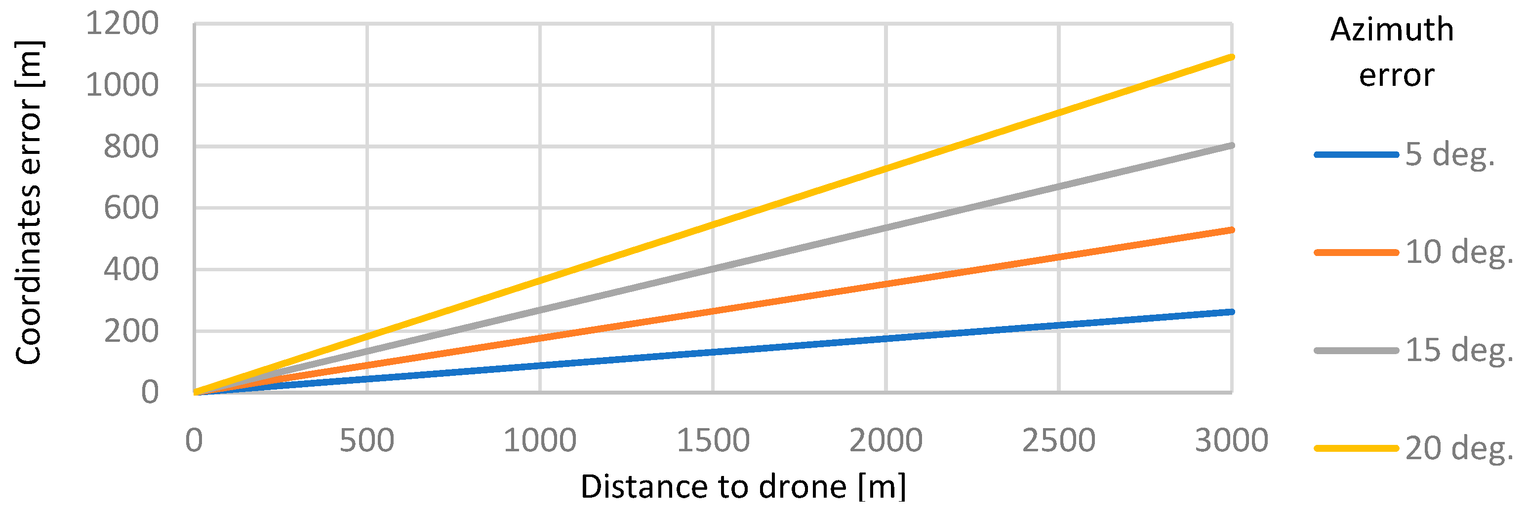
The azimuth misalignment of $5^0$ produces the drone coordinate error of about 87.5 m at a distance of 1 km (see Figure 5). It means that two radars will determine the coordinates of the same object differing by 87.5 m. As already mentioned, in mobile systems (especially on vehicles), it is difficult to obtain the radar azimuths alignment better than ${20}^0$. Then, the coordinates error will be 364 m (see Figure 5) at a distance of 1 km. Doubtlessly, this will disturb the proper operation of the system. Moreover, variable errors of azimuth measurement of both radars will cause a further increase in the drone position uncertainty. This is a quite serious issue and must be taken into account.

As was mentioned earlier, regarding a permanent system, the azimuths misalignment can be reduced using, for example, geodetic methods. However, radars in a mobile system can change location during the mission. Therefore, in new places, they must be aligned to the rest of the system as quickly as possible. To the best knowledge of the authors, this issue has not been described in publications yet (probably due to the commercial multi-radars mobile systems are still on low TRL). This statement is based on an unsuccessful search for a suitable method description. ‘Suitable’ means giving the desired accuracy at an acceptable time. However, the authors are conscious that this statement may be a kind of abuse. Research done by the authors shows that, at the moment, in practical applications, each of the radars is only roughly set separately using magnetic sensors and more advanced devices, such as gyrocompasses, GNSS RTK, or satellite compasses, are not applied in non-military mobile systems. Such a method does not ensure the desired accuracy.

This work presents a proposal to solve the problem of azimuths misalignment, consisting of the initial/coarse orientation of the radar system to the north using a magnetic compass, and then carrying out a calibration procedure consisting of automatically calculating corrections to azimuths measured by individual radars. The calibration process uses the "friend" drone flying in autonomous mode along a fixed route. The position of the drone does not have to be known, and the drone does not need to communicate with the system. The proposed method is simple, automatic, and requires no specialized knowledge. It gives very good results and can be successfully applied in real applications.

2. Proposed Method of Reducing the Azimuths Misalignment

In an ideal situation (no measurement errors), the coordinates of the drone detected by the radar are expressed by the following system of equations:

$$\{\begin{array}{l}{x}_{D\_ENU}=x_{R\_ENU}+D_{2D}·sin\left(A\right)\\ y_{D\_ENU}=y_{R\_ENU}+D_{2D}·cos\left(A\right)\end{array},$$

(1)

where:

$x_{D\_ENU},y_{D\_ENU}$	- true coordinates of the drone in the ENU system (East North Up),
$x_{R\_ENU},y_{R\_ENU}$	- true coordinates of the radar in the ENU system,
$D_{2D}$	- horizontal distance (2D) to the drone,
$A$	- azimuth of the drone from the radar position.

However, in real conditions, all quantities occurring on the right side of equations in the system (1) are affected by errors. Therefore, (1) will take the form

$$\{\begin{array}{l}{\widehat{x}}_{D\_ENU}=x_{R\_ENU}+{\delta }_{RP\_ENU}+\left(D_{2D}+{\delta }_{D\_2D}\right)·sin\left(A+{\delta }_{A\_ENU}\right)\\ {\widehat{y}}_{D\_ENU}=y_{R\_ENU}+{\delta }_{RP\_ENU}+\left(D_{2D}+{\delta }_{D\_2D}\right)·cos\left(A+{\delta }_{A\_ENU}\right)\end{array},$$

(2)

where:

${\delta }_{RP\_ENU}$	- radar coordinates determination error,
${\delta }_{D\_2D}$	- horizontal distance measurement error,
${\delta }_{A\_ENU}$	- azimuth measurement error in the ENU system.

Taking the practical experience in using FMCW radars for drone detection into consideration, it should be noted:

Note 1.: In practice, the radar position is fixed by GNSS before the operation and taken as a constant until the radar is moved to a new location. In such a case, ${\delta }_{RP\_ENU}$ is a constant error. It can be minimized by using Differential GNSS or GNSS RTK measurement techniques and by mounting the satellite system antenna centrally above the center of the radar measuring system. As already mentioned, the GNSS RTK technique is not used in commercial systems. A convenient solution is a Satellite Based Augmentation System (SBAS)—GNSS augmented by the differential system based on satellites. This reduces the radar position error to a sub-meter level. It allows omitting it in further considerations due to a small impact on the final performance of the proposed method.

Note 2.:${\delta }_{D\_2D}$ is a random variable with some small constant component resulting from the leveling of the mobile platform or mounting system of the radar. The constant component can be reduced almost to zero by using a leveling system and then ${\delta }_{D\_2D}$ can be modeled as an independent random variable with a normal standard distribution. Then, the highest probability density is concentrated around zero. Therefore, ${\delta }_{D\_2D}$ is also omitted in the proposed method.

Note 3.:${\delta }_{A\_ENU}$ is a random variable with a small variable component and a very large constant component, resulting from magnetic declination and magnetic deviation, radar and compass assembly on the platform, and the physical possibilities of setting the mobile platform or mounting system of the radar in the direction indicated by the magnetic compass. In practical applications, the variable component varies within $1^0-3^0$ (depending on the class of anti-drone radar), while the constant component can reach ${20}^0$. Such a large error in measuring the azimuth of the detected object will result in an error in determining its location (coordinates). According to Equation (2), it will be larger the greater the distance between the radar and the detected object is (see Figure 5). This will entail some complications, both in single- and multi-radar systems, which have already been mentioned in the Introduction.

Bearing in mind Notes 1 to 3, and that

$$A_m=A+{\delta }_{A\_ENU}\to A=A_m-{\delta }_{A\_ENU},$$

(3)

the system of Equation (1) can be written as

$$\{\begin{array}{l}{\widehat{x}}_{D\_ENU}={\widehat{x}}_{R\_ENU}+D_{m2D}·cos\left(A_m-{\delta }_{A\_ENU}\right)\\ {\widehat{y}}_{D\_ENU}={\widehat{y}}_{R\_ENU}+D_{m2D}·sin\left(A_m-{\delta }_{A\_ENU}\right)\end{array}.$$

(4)

This system has 3 unknowns: The estimated drone position in the ENU system $\left({\widehat{x}}_{D\_ENU},{\widehat{y}}_{D\_ENU}\right)$ and the azimuth measurement error in the ENU system $\left({\delta }_{A\_ENU}\right)$. The radar measurement results are the horizontal distance $\left(D_{m2D}\right)$ and the azimuth $\left(A_m\right)$, where

$$D_{m2D}=D_{m3D}·cos\left(E_m\right),$$

(5)

and:

$D_{m3D}$	- the spatial distance (3D) to the detected drone measured by the radar,
$E_m$	- the drone elevation measured by the radar or a priori assumed.

Estimated radar coordinates (fixed using DGNSS/SBAS measurement) in the ENU system $\left({\widehat{x}}_{R\_ENU},{\widehat{y}}_{R\_ENU}\right)$ are also known. On the left side of the equations, instead of true coordinates, there are their estimators, because both the position of the radar and the measurements are burdened with the errors. The errors were omitted in the system (4); however, they have an impact and cause some error in determining the coordinates of the detected drone.

From (4), it follows that unambiguous determination of unknowns based on measurements from a single radar is not possible. The next radar measurement will introduce the next 2 unknowns (new 2D coordinates of the drone), and 2 independent equations. Therefore, regardless of the number of measurements done by a single radar, the number of independent equations will always be 1 less than the number of unknowns.

Let us now consider a situation where a few radars in the network are tracking the same object. Then, the following system of independent equations can be formed

$$\{\begin{array}{c}{\widehat{x}}_{D\_ENU1}={\widehat{x}}_{R\_ENU1}+D_{m2D1}·cos\left(A_{m1}-{\delta }_{A\_ENU1}\right)\\ {\widehat{y}}_{D\_ENU1}={\widehat{y}}_{R\_ENU1}+D_{m2D1}·sin\left(A_{m1}-{\delta }_{A\_ENU1}\right)\\ ⋮\\ {\widehat{x}}_{D\_ENUn}={\widehat{x}}_{R\_ENUn}+D_{m2Dn}·cos\left(A_{mn}-{\delta }_{A\_ENUn}\right)\\ {\widehat{y}}_{D\_ENUn}={\widehat{y}}_{R\_ENUn}+D_{m2Dn}·sin\left(A_{mn}-{\delta }_{A\_ENUn}\right)\end{array},$$

(6)

where:

${\widehat{x}}_{D\_ENUi},{\widehat{y}}_{D\_ENUi}$	- the estimators of the drone true coordinates calculated on the base of measurements done by i-th radar,
${\widehat{x}}_{R\_ENUi},{\widehat{y}}_{R\_ENUi}$	- the estimators of the i-th radar true coordinates,
$D_{m2Di},A_{mi}$	- measurements results of horizontal distance and azimuth done by i-th radar,
$n$	- number of radars in the network.

Let us mark the position of the detected drone in the ENU system as ${\widehat{P}}_{D\_ENUi}$. This is the position estimated on the base of measurements done by i-th radar. Since both estimators of the radar coordinates and radar measurements are affected by errors, then

$${\widehat{P}}_{D\_ENU1}\ne {\widehat{P}}_{D\_ENU2}\ne \dots \ne {\widehat{P}}_{D\_ENUn}.$$

(7)

In this case, system (6) also has no unambiguous solution, because the number of unknowns will be $3n$, and the number of independent equations will be $2n$. However, due to all radars are observing the same object, we can assume a simplification:

$${\widehat{P}}_{D\_ENU1}={\widehat{P}}_{D\_ENU2}=\dots ={\widehat{P}}_{D\_ENUn}={\widehat{P}}_{D\_ENU}\left(x_{D\_ENU},y_{D\_ENU}\right),$$

(8)

and then, system (6) will take the following form:

$$\{\begin{array}{c}{x}_{D\_ENU}={\widehat{x}}_{R\_ENU1}+D_{m2D1}·cos\left(A_{m1}-{\delta }_{A\_ENU1}\right)\\ y_{D\_ENU}={\widehat{y}}_{R\_ENU1}+D_{m2D1}·sin\left(A_{m1}-{\delta }_{A\_ENU1}\right)\\ \hfill ⋮\hfill \\ x_{D\_ENU}={\widehat{x}}_{R\_ENUn}+D_{m2Dn}·cos\left(A_{mn}-{\delta }_{A\_ENUn}\right)\\ y_{D\_ENU}={\widehat{y}}_{R\_ENUn}+D_{m2Dn}·sin\left(A_{mn}-{\delta }_{A\_ENUn}\right)\end{array}.$$

(9)

In this situation, the number of unknowns will be $2+n$, and the number of independent equations $2n$, and already for $n=2$, all 3 unknowns can be fixed. However, for $n>2$, redundant equations will appear. In such a case, we have $\left(\begin{array}{c}2+n\\ 2n\end{array}\right)$ numbers of possible equations combinations, which give a solution in the form of $S\left({\widehat{P}}_{D\_ENU},{\widehat{\delta }}_{A\_ENU1},\dots ,{\widehat{\delta }}_{A\_ENUn}\right)$. Unfortunately, due to errors both in the estimated coordinates of the radar position and in the radar measurements, each of these combinations will give a slightly different solution. These differences will depend not only on the radar coordinates errors and the azimuth, elevation, and distance measurement errors but also on the relative location of the radars and the detected object (the system geometry described by the dilution of precision coefficient). It should be noted that the geometry of the system will change during the drone’s flight. Therefore ${\delta }_{A\_ENUi}$ calculated for the moment $t$, based on observations from $n$ radars, can be expressed by the following equation:

$${\delta }_{A\_ENUi}\left(t\right)={\delta }_{A\_ENUi}^{const}+{\delta }_{A\_ENUi}^{var}={\delta }_{A\_ENUi}^{const}+f\left({\delta }_{A\_ENU1}\left(t\right),\dots ,{\delta }_{A\_ENUn}\left(t\right),{\delta }_A^{DOP}\left(t\right)\right),$$

(10)

where:

${\delta }_{A\_ENUi}^{const}$	- constant component of ${\delta }_{A\_ENUi}\left(t\right)$,
${\delta }_{A\_ENUi}^{var}$	- variable in time component of ${\delta }_{A\_ENUi}\left(t\right)$,
${\delta }_A^{DOP}\left(t\right)$	- variable in time component of ${\delta }_{A\_ENUi}\left(t\right)$ resulting from the changing geometry of the radars-detected object arrangement due to drone flight.

${\delta }_{A\_ENUi}^{const}$ is the sought difference between the radar north and the true north:

$$Nort{h}_{real}+{\delta }_{A_{ENUi}}^{const}=Nort{h}_{RADARi}\to {\delta }_{A\_ENUi}^{const}=Nort{h}_{RADARi}-Nort{h}_{real}.$$

(11)

Due to ${\delta }_{A\_ENUi}^{const}\gg {\delta }_{A\_ENUi}^{var}$, the determination of $Nort{h}_{RADARi}$ would significantly improve both the accuracy of determining the coordinates of the detected object and minimize the likelihood of classifying a single drone as a swarm and vice versa. Both factors are crucial for the anti-drone system. The calculated ${\delta }_{A\_ENUi}^{const}$ value with the opposite sign would be a correction to the measured azimuth by the radar and could be automatically taken into account by the master system responsible for the multi-sensors data fusion. In the proposed method, determining the difference $Nort{h}_{RADARi}-Nort{h}_{real}$, and hence the correction for measuring azimuths consists of eliminating the ${\delta }_{A\_ENUi}^{var}$ component from Equation (10). According to the proposed idea, this is done by multi-radars observations of a flying drone with unknown coordinates. Azimuth measurement error ${\delta }_{A\_ENU}$ is estimated in every measurement epoch $\left(t_e\right)$, and then the constant component of the azimuth measurement error is calculated as:

$${\delta }_{A\_ENU}^{const}=\frac{1}{m}{\displaystyle \sum }_{j=1}^m{\delta }_{A\_ENU}\left(t_{ej}\right),$$

(12)

where:

$m$	- number of measurement epochs common to all radars,
${\delta }_{A\_ENU}\left(t_{ej}\right)$	- azimuth measurement error at the moment $\left(t_{ej}\right)$.

Therefore, the key issue is to estimate the azimuth measurement error ${\delta }_{A\_ENU}$ in every measurement epoch. In the proposed method, instead of the classical form of system of equations describing the coordinates of the detected object (9), the following form is used:

$$\{\begin{array}{c}{D}_{m2D1}=\sqrt{{\left(x_{D\_ENU}-{\widehat{x}}_{R\_ENU1}\right)}^2+{\left(y_{D\_ENU}-{\widehat{y}}_{R\_ENU1}\right)}^2}\\ A_{m1}=arctan\left(\frac{x_{D\_ENU1}-{\widehat{x}}_{R\_ENU1}}{y_{D\_ENU1}-{\widehat{y}}_{R\_ENU1}}\right)+{\delta }_{A\_ENU1}\\ ⋮\\ D_{m2Dn}=\sqrt{{\left(x_{D\_ENU}-{\widehat{x}}_{R\_ENUn}\right)}^2+{\left(y_{D\_ENU}-{\widehat{y}}_{R\_ENUn}\right)}^2}\\ A_{mn}=arctan\left(\frac{x_{D\_ENU}-{\widehat{x}}_{R\_ENUn}}{y_{D\_ENU}-{\widehat{y}}_{R\_ENUn}}\right)+{\delta }_{A\_ENUn}\end{array}.$$

(13)

Let us assume the approximate drone position and mark it as $P_{D\_ENU}^0\left(x_{D\_ENU}^0,y_{D\_ENU}^0\right)$. Let it be a position calculated on the basis of observations from any one radar from the network:

$$\{\begin{array}{l}{x}_{D\_ENU}^0={\widehat{x}}_{R\_ENUi}+D_{m2Di}·cos\left(A_{mi}\right)\\ y_{D\_ENU}^0={\widehat{y}}_{R\_ENUi}+D_{m2Di}·sin\left(A_{mi}\right)\end{array}.$$

(14)

Now let us expand the right sides of the equations of the system (13) in the Taylor series relative to $P_{D\_ENU}^0$, limiting to the second order components:

$$\{\begin{array}{c}{D}_{m2D1}=D_{m2D1}^0+\frac{\partial }{\partial x_{D\_ENU}^0}\left(D_{m2D1}^0\right)·\Delta x_{D\_ENU}+\frac{\partial }{\partial y_{D\_ENU}^0}\left(D_{m2D1}^0\right)·\Delta y_{D\_ENU}\\ A_{m1}-{\delta }_{A\_ENU1}=A_{m1}^0+\frac{\partial }{\partial x_{D\_ENU}^0}\left(A_{m1}^0\right)·\Delta x_{D\_ENU}+\frac{\partial }{\partial y_{D\_ENU}^0}\left(A_{m1}^0\right)·\Delta y_{D\_ENU}\\ \hfill ⋮\hfill \\ D_{m2Dn}=D_{m2Dn}^0+\frac{\partial }{\partial x_{D\_ENU}^0}\left(D_{m2Dn}^0\right)·\Delta x_{D\_ENU}+\frac{\partial }{\partial y_{D\_ENU}^0}\left(D_{m2Dn}^0\right)·\Delta y_{D\_ENU}\\ A_{mn}-{\delta }_{A\_ENUn}=A_{mn}^0+\frac{\partial }{\partial x_{D\_ENU}^0}\left(A_{mn}^0\right)·\Delta x_{D\_ENU}+\frac{\partial }{\partial y_{D\_ENU}^0}\left(A_{mn}^0\right)·\Delta y_{D\_ENU}\end{array},$$

(15)

wherein:

$$D_{m2Di}^0=\sqrt{{\left(x_{D\_ENU}^0-{\widehat{x}}_{R\_ENUi}\right)}^2+{\left(y_{D\_ENU}^0-{\widehat{y}}_{R\_ENUi}\right)}^2},$$

(16)

$$A_{mi}^0=arctan\left(\frac{x_{D\_ENU}^0-{\widehat{x}}_{R\_ENUi}}{y_{D\_ENU}^0-{\widehat{y}}_{R\_ENUi}}\right).$$

(17)

Let’s mark the individual derivatives as follows:

$$\frac{\partial }{\partial x_{D\_ENU}^0}\left(D_{m2Di}^0\right)=m_{Dxi},\frac{\partial }{\partial y_{D\_ENU}^0}\left(D_{m2Di}^0\right)=m_{Dyi},$$

$$\frac{\partial }{\partial x_{D\_ENU}^0}\left(A_{mi}^0\right)=m_{Axi},\frac{\partial }{\partial y_{D\_ENU}^0}\left(A_{mi}^0\right)=m_{Ayi}.$$

Then, the system of Equation (15) will take the form

$$\{\begin{array}{c}{D}_{m2D1}-D_{m2D1}^0=m_{Dx1}·\Delta x_{D\_ENU}+m_{Dy1}·\Delta y_{D\_ENU}\\ A_{m1}-A_{m1}^0=m_{Ax1}·\Delta x_{D\_ENU}+m_{Ax1}·\Delta y_{D\_ENU}+{\delta }_{A\_ENU1}\\ ⋮\\ D_{m2Dn}-D_{m2Dn}^0=m_{Dxn}·\Delta x_{D\_ENU}+m_{Dyn}·\Delta y_{D\_ENU}\\ A_{mn}-A_{mn}^0=m_{Axn}·\Delta x_{D\_ENU}+m_{Axn}·\Delta y_{D\_ENU}+{\delta }_{A\_ENUn}\end{array}.$$

(18)

The system of Equation (18) can be written in matrix form as

$$\begin{array}{ccc}{\left[\begin{array}{c}{D}_{m2D1}-D_{m2D1}^0\\ \begin{array}{c}{A}_{m1}-A_{m1}^0\\ D_{m2D2}-D_{m2D2}^0\\ A_{m2}-A_{m2}^0\end{array}\\ \begin{array}{c}⋮\\ D_{m2Dn}-D_{m2Dn}^0\\ A_{mn}-A_{mn}^0\end{array}\end{array}\right]}_{2n\times 1}& ={\left[\begin{array}{ccccccc}{m}_{Dx1}& m_{Dy1}& & 0& 0& \cdots & 0\\ m_{Ax1}& m_{Ay1}& & 1& 0& \cdots & 0\\ m_{Dx2}& m_{Dy2}& & 0& 0& \cdots & 0\\ m_{Ax2}& m_{Ay2}& & 0& 1& \cdots & 0\\ & & ⋮& & \\ m_{Dxn}& m_{Dyn}& & 0& 0& \cdots & 0\\ m_{Axn}& m_{Ayn}& & 0& 0& \cdots & 1\end{array}\right]}_{2n\times (n+2)}& ·{\left[\begin{array}{c}\Delta x_{D_{ENU}}\\ \Delta y_{D_{ENU}}\\ {\delta }_{A_{ENU1}}\\ {\delta }_{A_{ENU2}}\\ ⋮\\ {\delta }_{A_{ENUn}}\end{array}\right]}_{\left(n+2\right)\times 1}\\ \mathbf{d}& \mathbf{A}& \mathbf{X}\end{array}.$$

(19)

$X$ is a vector of unknowns. Estimated value of $X$ using least square estimator is:

$$\widehat{X}={\left(A^{\mathit{T}}A\right)}^{-1}{A}^{\mathit{T}}d.$$

(20)

The solution of (20) is:

$$\widehat{X}={\left[\begin{array}{c}\Delta {\widehat{x}}_{D\_ENU}\\ \Delta {\widehat{y}}_{D\_ENU}\\ {\widehat{\delta }}_{A\_ENU1}\\ {\widehat{\delta }}_{A\_ENU2}\\ ⋮\\ {\widehat{\delta }}_{A\_ENUn}\end{array}\right]}_{\left(n+2\right)\times 1}.$$

(21)

Using $\Delta {\widehat{x}}_{D\_ENU},\Delta {\widehat{y}}_{D\_ENU}$, the estimated position of the drone can be calculated as:

$$\begin{gathered} {\widehat{x}}_{D\_ENU}=x_{D\_ENU}^0+\Delta {\widehat{x}}_{D\_ENU}, \\ {\widehat{y}}_{D\_ENU}=y_{D\_ENU}^0+\Delta {\widehat{y}}_{D\_ENU}. \end{gathered}$$

(22)

If $\Delta {\widehat{x}}_{D\_ENU}>1m$ or $\Delta {\widehat{y}}_{D\_ENU}>1m$, the next iteration is necessary, taking the estimated drone position calculated from (22) as the new approximate position. The final value of the azimuth measurement error for each of the radars is the value of ${\widehat{\delta }}_{A\_ENUi}$ from the last iteration. Then, the ${\widehat{\delta }}_{A\_ENU}^{const}$ value is calculated based on (12). According to the presented idea the correction to measuring azimuths (the difference between the true north and the radar north) for a given radar is:

$$c_{Ai}=-{\widehat{\delta }}_{A\_ENUi}^{const}.$$

(23)

Then, the azimuth estimator of the detected object for a given radar is:

$${\widehat{A}}_i=A_{mi}+c_{Ai}.$$

(24)

The practical implementation of the proposed method can be presented in the form of the following algorithm:

BEGIN //drone started a calibration flight and all radars detected a drone

j := 0; //first measurements epoch

n := number of radars;

REPEAT

FOR i := 1 TO n DO

Get the radars measurements $M_i=\left\{A_{mi},D_{m2Di}\right\}$;

Bring $M_i$ to a common moment $\left(t_{ej}\right)$; //explanation below the algorithm

Compute ${\widehat{\delta }}_{A\_ENU}\left(t_{ej}\right)$ for all radars;  //using Equation (20)

j := j + 1;              //next measurement epoch

UNTIL drone ended a calibration flight

m := j;                  //number of measurements epoch

Computation of ${\delta }_{A\_ENU}^{const}$;         //using Equation (12)

END.

Since observations of the drone by each of the radars are generally not done at the same time, but in some time window (approximately equal to the period of scanning of a particular radar), the values of measured azimuths and distances must be brought to a common moment $\left(t_e\right)$. The proposed method uses linear interpolation between the measurements immediately preceding and following $\left(t_e\right)$, according to the formulas:

$$\begin{gathered} {\widehat{A}}_m\left(t_e\right)=A_m\left(t_0\right)+\frac{t_e-t_0}{t_1-t_0}\left(A_m\left(t_1\right)-A_m\left(t_0\right)\right), \\ {\widehat{D}}_{m2D}\left(t_e\right)=D_{m2D}\left(t_0\right)+\frac{t_e-t_0}{t_1-t_0}\left(D_{m2D}\left(t_1\right)-D_{m2D}\left(t_0\right)\right), \end{gathered}$$

(25)

where:

$t_0$	- the time immediately preceding $\left(t_e\right)$, when the measurement was done,
$t_1$	- the time immediately following $\left(t_e\right)$, when the measurement was done,
${\widehat{A}}_m\left(t_e\right),{\widehat{D}}_{m2D}\left(t_e\right)$	- estimated values of azimuth and distance at moment $\left(t_e\right)$,
$A_m\left(t_0\right)$, $A_m\left(t_1\right)$	- measured azimuths at moments $\left(t_0\right)$ i $\left(t_1\right)$,
$D_{m2D}\left(t_0\right)$, $D_{m2D}\left(t_1\right)$	- measured distances at moments $\left(t_0\right)$ i $\left(t_1\right)$.

3. Method of Verification

Intensive numerical simulations were performed to verify the correctness of the developed method. There were simulated drone flights along a fixed route and indications of FMCW radars tracking them—measurements of azimuth and distance. The simulation software SimWizardADS developed by the Polish company Basic Solution was used in the research. The software was developed as part of a project granted by the Polish National Center for Research and Development (NCRD) in 2017 under the name SimWizardSSAD. The software was accepted by NCRD experts as a reliable tool for simulation of anti-drone systems in the scope of detection and is being further developing under the name SimWizardADS. An example of the simulation wizard window is shown in Figure 6.

The numerical simulations were performed with the following assumptions:

• Number of the simulations: 95,000
• In each simulation, an anti-drone system consisting of 3 and 4 omnidirectional long-range radars will be simulated. The radars will measure distances and azimuths without elevations (2D radars):
  • In the variant with 3 radars, they will be located in the nodes of an equilateral triangle. The side length will be 2 km (see Figure 7-left),
  • In the variant with 4 radars, they will be located in the nodes of the rectangle. The side length will be 2 km (see Figure 7-right),
  • Detection range of the radars will be 2.5 km,
  • The beam width of the radars in the elevation will be ${10}^0$. Due to the fact that the radars do not measure the height of the detected object, it is assumed that it equals half the beam width. As mentioned earlier, this is a common assumption in 2D radars,
  • Range measurement errors will contain only the variable component. It will be generated randomly according to the normal distribution. In each simulation, each radar will be assigned a standard deviation of the range measurement error (RMS range). It will be selected randomly (for each radar independently) from a set of 0.6, 0.8, 1.0, or 1.2 m. These are typical values of the RMS range for anti-drone FMCW radars available on the commercial (open) market. The values will be constant for one simulation. In the next one, the new values will be drawn on the same rules,
  • Azimuth measurement errors will contain a variable and constant component. The variable component will be generated randomly according to the normal distribution. In each simulation, a standard deviation of azimuth measurement error (RMS azimuth) will be assigned to each radar. It will be selected randomly (for each radar independently) from a set of 0.8, 1.0, 1.2, or 1.4 m. These are typical RMS azimuth values for anti-drone FMCW radars available on the commercial (open) market. The values will be constant for one simulation. The next one will draw new values on the same principles,
  • The constant component of the azimuth measurement error will be randomly generated according to a uniform distribution in the range of +/− ${15}^0$. The values will be generated independently for each radar and will be constant for one simulation. In the next one, new values will be drawn on the same rules,
  • The radar scanning frequency will be 2, 1, 1.5, or 0.5 Hz. These are typical values for anti-drone FMCW radars available on the commercial (open) market. The values will be chosen randomly and will be constant for one simulation. In the next one, new values will be drawn on the same principles.
• The calibration flight (using "friend" drone) will take place along the routes shown in Figure 8. The height will be 20 m above the ground. The justification for the route selection can be found below. The drone speed will be constant and equal to 10 m/s. This is a typical value for commercial drones. This means that the calibration flight will take 11 min 10 s for the variant with 3-radars and 10 min 40 s for the 4-radars option.
• The analysis of the simulation results will be carried out in the context of:
  • Calibration accuracy. The measure will be the difference between the radar north and the true north after calibration,
  • The radar north increasing. A measure will be a value of which a difference between the radar north and the true north has changed,
  • For each of the value listed in part 4, the following parameters will be computed:
  • Mean value,
  • Standard deviation (RMS),
  • Absolute minimum and maximum values and parameters at which they occurred (radar configuration, actual radar north deviation from the true north, and a standard deviation of azimuth and distance measurement.

Experiences of the authors with commercial FMCW radars used in anti-drone systems indicate that when choosing a calibration flight route, certain factors should be considered. They result from the characteristics of commercial FMCW radars used in anti-drone systems. The idea is to minimize the likelihood of losing drone tracking, as this will adversely affect the effectiveness of the proposed method. At the same time, the likelihood of various random measurement errors associated with the mutual geometry between the drone and the radars should be maximized. Practical experiences show that:

• The route, if possible, should be in a common coverage area for all radars. This will have a positive effect on the accuracy of the proposed method. In such a case, the system of observational equations will contain more redundant equations. It will increase the accuracy of the estimator of the azimuth measurement error for individual radars.
• Commercial FMCW radars have difficulties with detecting and tracking low radial-speed objects (slowly approaching or moving away from the radar). Therefore, the calibration route should not include sections with a low radial-speed relative to any radar.
• The accuracy of measuring horizontal distances by 2D radars decreases with increasing distance to the object, as the difference between the assumed and actual height of the drone increases (see Figure 5). Therefore, the flight should be at a minimum safe altitude. Then, the 3D and 2D distances will be close to each other, which will minimize the error associated with the uncertainty of the drone elevation. Practice shows that 20 m height is the optimal solution.
• Measurement experiments with FMCW radars indicate that the accuracy of the determined drone parameters also depends on the flight direction relative to the radar (among others, due to the different position of the drone’s hull relative to the radar, and thus different RCS). Therefore, the calibration flight route should include sections where the drone is approaching and moving away from the radar.
• The route should not be too long, as this will make the calibration process time consuming, and at the same time, should consider points 1–4 as much as possible.

Taking the above into account, several possible variants of calibration flight routes were analyzed. It was finally found that the optimal ones (for selected locations of the radars) will be as shown in Figure 7.

4. Results

According to the assumptions, 95,000 simulations were performed for each of the two variants of the radar location (the 3- and 4-radars variants).

Table 1. Calibration accuracy in the network system consisting of 3 radars.

Measure	Radar 1	Radar 1	Radar 3
Mean Value	$-{0.24}^0$	${0.23}^0$	$0^0$
Standard Deviation	${3.42}^0$	${3.36}^0$	${3.31}^0$
Min Value (the best)	$0^0$	$0^0$	$0^0$
Max Value (the worst)	${9.49}^0$	${8.99}^0$	${8.75}^0$

and

Table 2. Calibration accuracy in the network system consisting of 4 radars.

Measure	Radar 1	Radar 1	Radar 3	Radar 4
Mean Value	$-{0.09}^0$	$-{0.04}^0$	${0.02}^0$	$-{0.08}^0$
Standard Deviation	${3.40}^0$	${3.79}^0$	${3.12}^0$	${3.32}^0$
Max Value (the best)	$0^0$	$0^0$	$0^0$	$0^0$
Min Value (the worst)	${9.73}^0$	${10.86}^0$	${8.60}^0$	${9.46}^0$

show the calibration accuracy obtained due to the proposed method. The measure used is the difference between the radar north and the true north after calibration.

As it results from the data presented in Table 1 and Table 2, the average value of the constant component of the azimuth error after calibration is close to 0 for each of the radars in the network, both in the case of the system consisting of 3 and 4 radars. In the best cases, it has been eliminated. However, in the worst cases, after calibration, it was still around $9-{10}^0$. 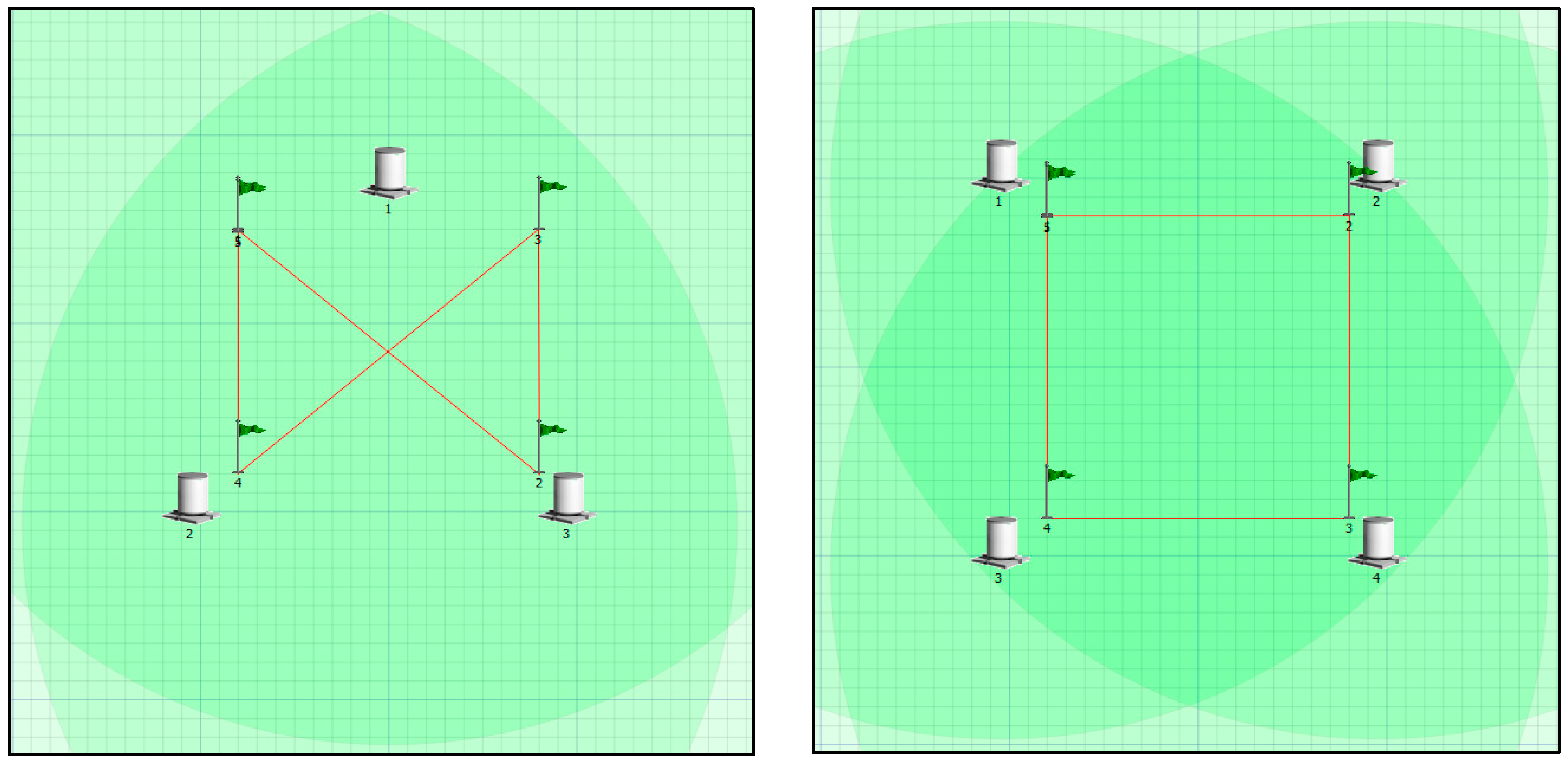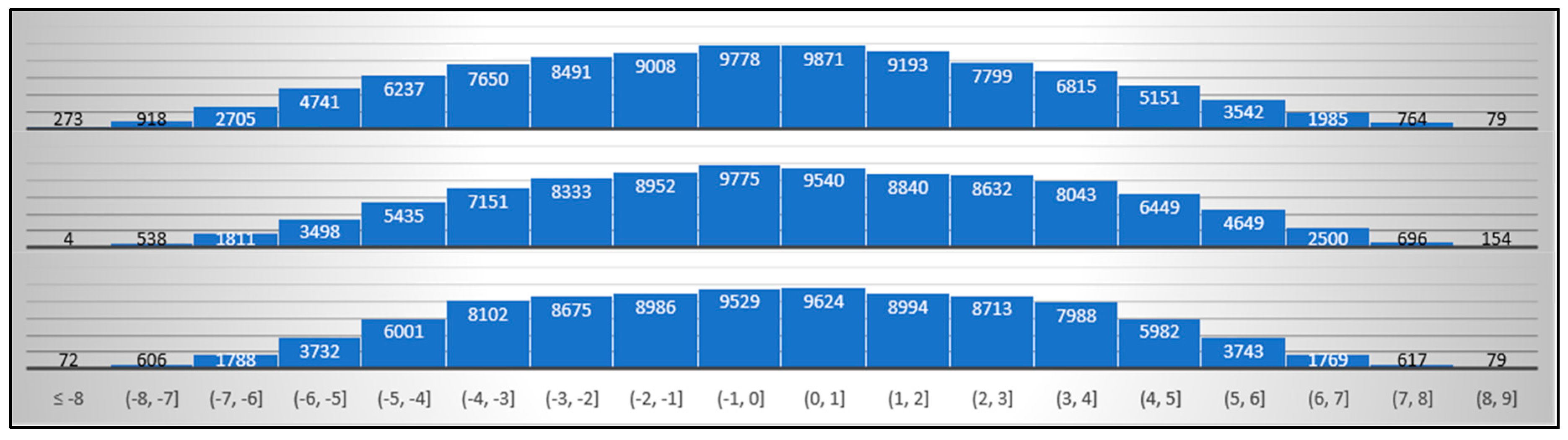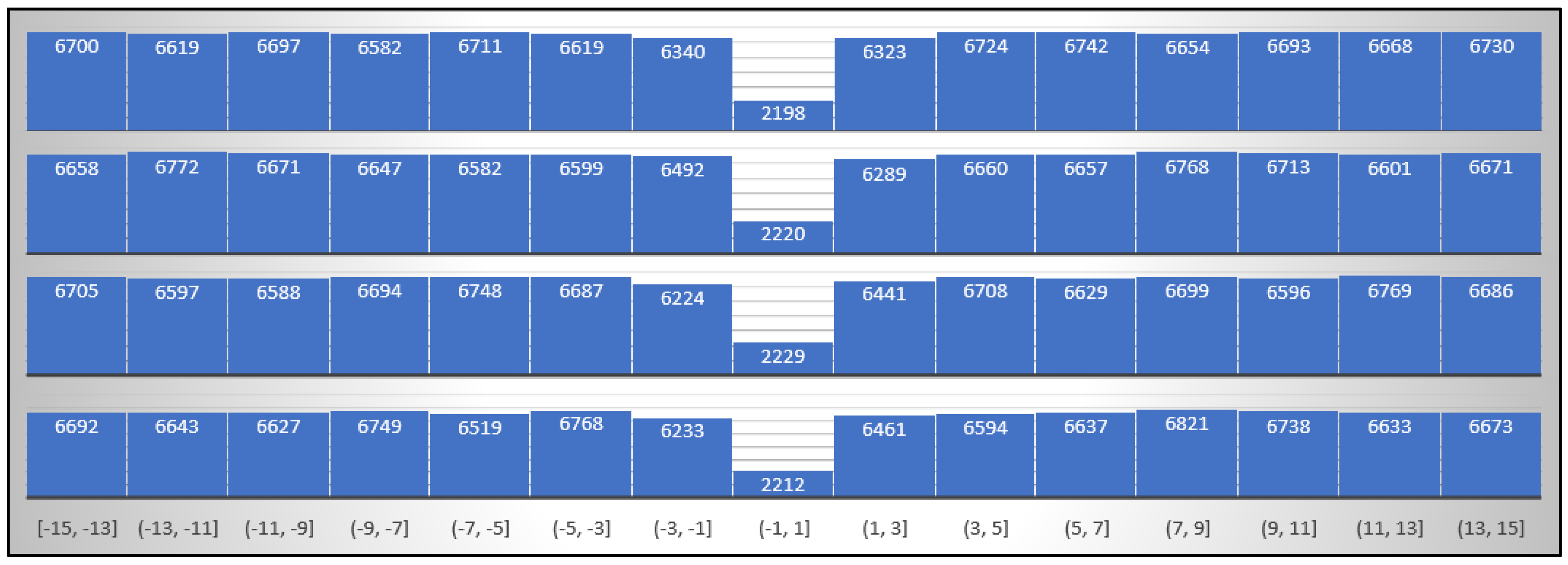Therefore, to better analyze the effectiveness of the proposed method, Figure 8 presents histograms of the azimuth error constant component for radars R1, R2, and R3 in the 3-radars network (see Figure 7 (left)) before and Figure 9 after calibration. On the horizontal axis of the charts, there are ranges of the azimuth error constant component in degrees, and the numbers in the blue rectangles are the numbers of individual ranges.

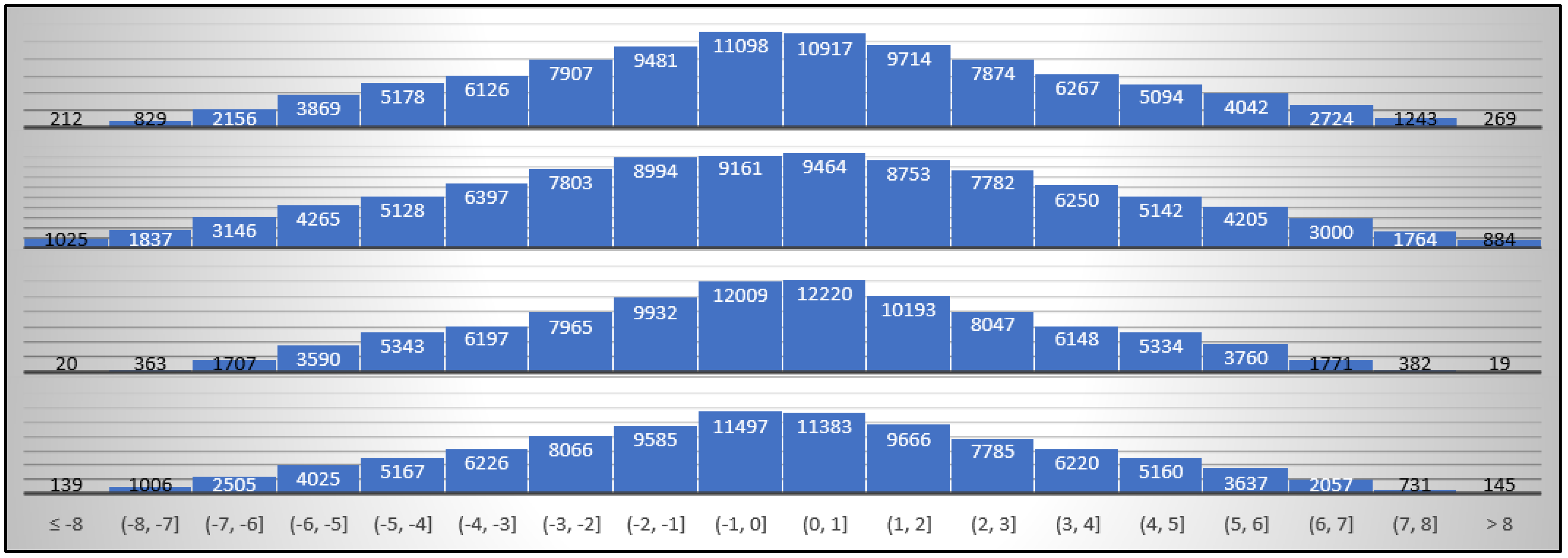
Figure 8 and Figure 9 show that for each of the radars, there was a clear improvement—a decrease in the value of the constant component of the azimuth error. Moreover, before calibration, the errors had a uniform distribution (according to the simulation assumptions), while after calibration, it was similar to the Gaussian distribution, with the highest probability density centered around 0. It is worth noting that only about 5% percent of errors after calibration exceeded the value of $6^0$, which should be considered a very good result, given that before calibration, such errors were about 65%. It is also apparent from Figure 8 and Figure 9 that the method impacts on a constant azimuth measurement error for each of the radars in a similar way. The same is also true in the 4-radars network (shown in Figure 7 (right)). Histograms of the azimuth error constant component for radars R1, R2, R3, and R4 before calibration are shown in Figure 10 and after calibration in Figure 11.

It can be seen in Figure 8, Figure 9, Figure 10 and Figure 11 that the azimuth error constant component before and after calibration for both 3- and 4-radars networks have similar distributions. Therefore, the results of further analyses are presented based on one selected radar from both tested cases. The solution was applied to limit the volume of the paper. To maintain proper reliability, the results of the analyses are presented for the worst case (least improvement and greatest deterioration after calibration). This was the case of R1 radar from the 4-radars network (see Figure 7 (right)).

The graphs in Figure 8, Figure 9, Figure 10 and Figure 11 show that the proposed method significantly improves the accuracy of the azimuth measurement by reducing azimuths misalignment (decreasing the constant error of the azimuths measurements). However, the distribution of the azimuth error constant component after calibration does not yet give a complete picture of the method’s effectiveness. There are no answers to the following important questions:

a)

Is there radar orientation improvement in each of the cases, or are there cases where the value of the azimuth error constant component increases after calibration?

b)

If there are cases of radar orientation deterioration relative to the north after calibration, how large are they, and do they preclude the practical application of the proposed method?

c)

What is the percentage of the radar orientation relative to the north improvement, in comparison to the initial value of the azimuth error constant component?

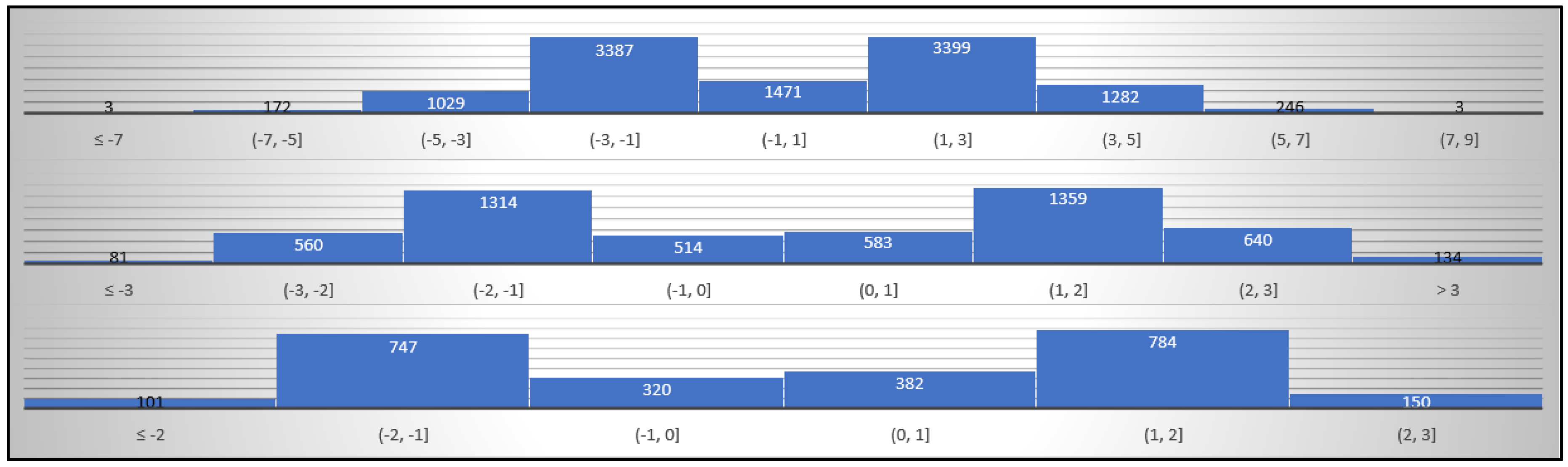
To answer the above questions, an analysis of the radar north improvement was performed. The measure used was the value by which the difference between the radar north and the true north changed due to calibration. To better show the effect of the proposed method, the radar north improvement was expressed as a percentage of the constant azimuth error before calibration. The results of the analysis for the selected radar (the worst case) are presented in Figure 12, Figure 13 and Figure 14.

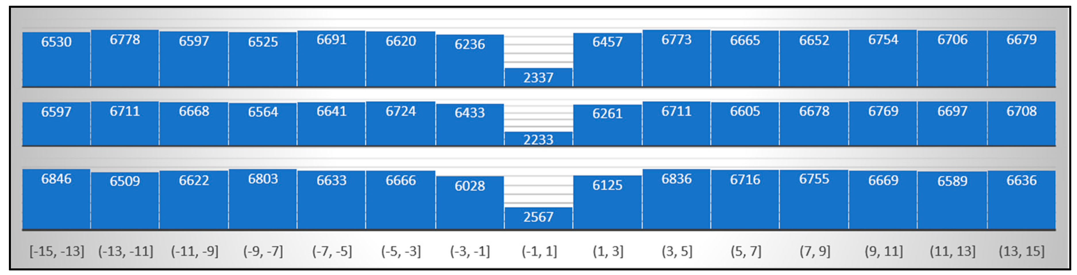
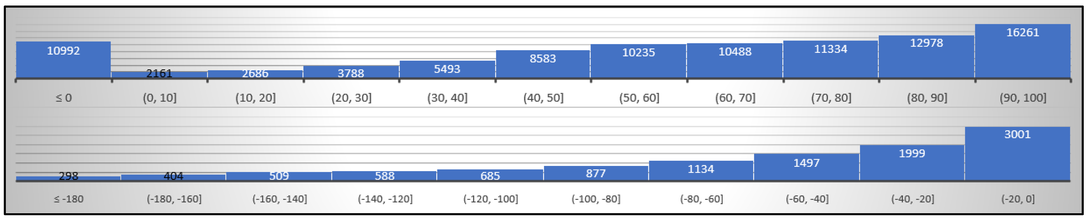
Figure 12 shows the percentage histogram of improvement and deterioration of the selected radar orientation relative to the north. The horizontal axis presents the percentages, and the numbers in the blue rectangles are the number of individual ranges. A negative percentage value ($\le 0$) means that after calibration, the radar orientation has deteriorated.

Figure 12 shows that up to 11.6% of cases, after calibration by the proposed method, the radar orientation deteriorated relative to the true north. Most values of degradation did not exceed 100% of the pre-calibration value, but there were also cases where they reached 200%. At first glance, this seemed very worrying, because even a 20% deterioration may be unacceptable if it concerns large initial values (before calibration). Therefore, it seems to be important to answer the following questions:

a)

How big is the deterioration in numerical values?

b)

Does it concern small or large values of initial orientation errors?

c)

How this might affect the practical application of the proposed method?

To answer them, deterioration cases were thoroughly analyzed. Figure 13 shows the histogram of the initial (before calibration) constant azimuth errors for the R1 radar in the 4-radars system, where the orientation was deteriorated after the calibration.

Figure 13 shows that the large percentage deterioration of radar orientation relative to the north was related to small initial values (before calibration). The deterioration by more than 50% basically concerned angles not greater than $3^0$, and 100 not greater than $2^0$. This means that even in the worst case of deterioration, the azimuth misalignment after calibration did not exceed $4^0$, which is completely acceptable from a practical point of view. Moreover, it should be emphasized that in all analyzed cases, the deterioration of radar orientation relative to true north after calibration, concerned only one radar in the network, while significantly improving the orientation of the other radars. The deterioration effect occurred when one radar had a small initial error and the rest had large ones.

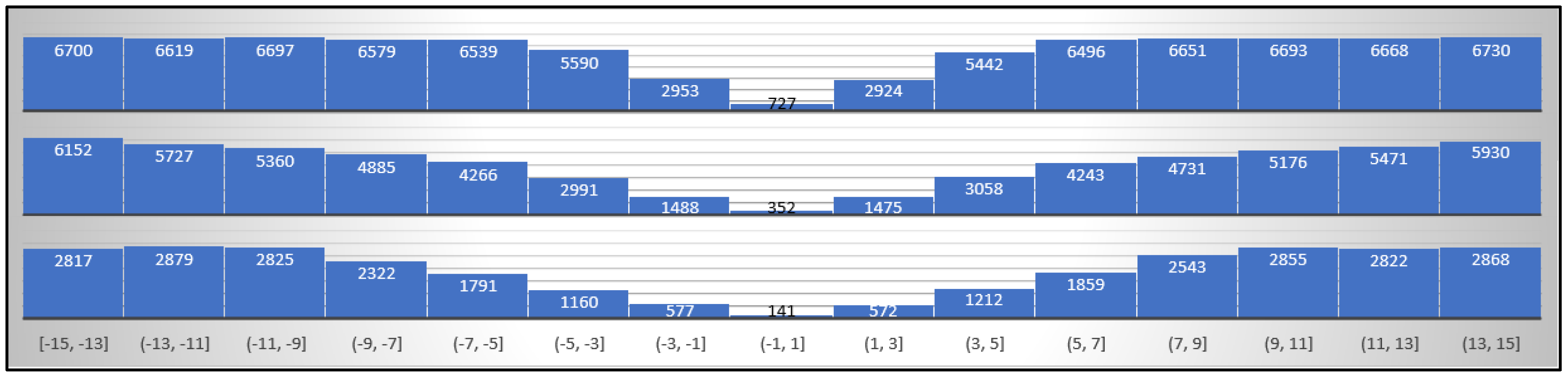
To show the advantages of the proposed method for the same radar, the results of an analogous analysis regarding the improvement of orientation relative to true north are presented below. Figure 14 shows the distribution of the initial (before calibration) azimuth constant errors for which the R1 radar orientation improved.

The graphs shown in Figure 14 show the advantages of the proposed calibration method. It can be seen that the method improves the initial orientation of the radar relative to the north over the entire range of initial errors. It is the most effective for errors above $3^0$.

5. Discussion

Based on the obtained results, one can say:

• The method improves the orientation of radars relative to the true north over the entire range of initial errors (before calibration). It is especially effective if they are above $3^0$. Moreover, the method reduces the initial value of the error, the higher it is. This is of great practical importance, as it greatly reduces the error in determining the coordinates of the detected object by the radar. What is more, the method only requires a very coarse orientation of the radars to the north (e.g., using magnetic compass indications), which is also important in real applications, as it does not require the use of specialized equipment and significantly reduces the time needed to prepare the system for operation. The smallest improvement in the radar orientation occurs for angles below $3^0$, which is not a practical problem.
• Not always does the proposed method improve the initial value of the radar orientation. In about 10% of cases, deterioration occurs. However, it concerns small initial errors (below $3^0$). As a result, after calibration, the azimuth misalignment did not exceed $4^0$. This is perfectly acceptable from a practical point of view, because in all registered cases, the deterioration concerned only one radar in the network, while significantly improving the orientation of the others.
• Further work will focus on improving the method’s effectiveness. It is planned to use another method of calculating the initial position of the drone for the first iteration purposes. It was noted that the unfavorable results might be due to the fact that the approximate position was too far from the true one. Moreover, it should be checked whether weighing the measurements (depending on the azimuth and distance measurement accuracy) will significantly improve the calibration accuracy, or whether the increase will be insignificant and only the computational complexity will increase. Further research is also planned to look for the optimal calibration flight route. It would be desirable to achieve maximum calibration accuracy while minimizing flight length.

6. Conclusions

The proposed method of calibration improves the initial orientation of the radars relative to the north over the entire range of the initial errors. Moreover, it reduces the azimuth misalignment the bigger its initial value is. This is an undoubted advantage of the method and also has a great practical meaning, as it leads to a significant reduction of errors in determining the coordinates of the detected object (see Figure 5). Although there are cases when the azimuths misalignment increased after calibration, it has no practical meaning as it only concerned small initial errors. Therefore, after calibration, the orientation errors were still acceptable. The disadvantage of the method may be the need to perform a drone calibration flight along a fixed route. However, this appears to be a minor nuisance compared to other calibration methods.

References

1. Goldman Sachs. Available online: https://www.goldmansachs.com/our-thinking/technology-driving-innovation/drones/ (accessed on 11 August 2019).
2. Interesting Engineering. Available online: https://interestingengineering.com/top-5-drone-intercepting-methods-you-should-know-about (accessed on 11 August 2019).
3. Michel, A.H. Counter-Drone Syst; The report by Bard College’s Center for the Study of the Drone; Bard College’s Center for the Study of the Drone: Dutchess Country, NY, USA, 2018. [Google Scholar]
4. Hertz Systems. Available online: http://thehawksystem.com/pl/ (accessed on 1 September 2019).
5. SpotterRF. Available online: https://spotterrf.com/products/mobile-solutions/ (accessed on 1 September 2019).
6. Farlik, J.; Kratky, M.; Casar, J.; Stary, V. Multispectral Detection of Commercial Unmanned Aerial Vehicles. Sensors 2019, 19, 1517. [Google Scholar] [CrossRef] [PubMed]
7. Laurenzis, M.; Hengy, S.; Hommes, A.; Kloeppel, F.; Shoykhetbrod, A.; Geibig, T.; Johannes, W.; Naz, P.; Christnacher, F. Multi-sensor field trials for detection and tracking of multiple small unmanned aerial vehicles flying at low altitude. In Proceedings of the Signal Processing, Sensor/Information Fusion, and Target Recognition XXVI, Anaheim, CA, USA, 10–12 April 2017. [Google Scholar]
8. Nassi, B.; Shabtai, A.; Masuoka, R.; Elovici, Y. SoK—Security and Privacy in the Age of Drones: Threats, Challenges, Solution Mechanisms, and Scientific Gaps. arXiv 2019, arXiv:1903.05155. [Google Scholar]
9. Doroftei, D.; De Cubber, G. Qualitative and quantitative validation of drone detection systems. In Proceedings of the International Symposium on Measurement and Control in Robotics, Mons, Belgium, 26–28 September 2018. [Google Scholar] [CrossRef]
10. Zhahir, A.; Razali, A.; Mohd Ajir, M.R. Current development of UAV sense and avoid system. IOP Conf. Ser. Mater. Sci. Eng. 2016, 152, 012035. [Google Scholar] [CrossRef]
11. Eriksson, N. Conceptual Study of a Future Drone Detection System. Master’s Thesis, Product Development, Chalmers University of Technology, Gothenburg, Sweden, 2018. [Google Scholar]
12. Hommes, A.; Shoykhetbrod, A.; Noetel, D.; Stanko, S.; Laurenzis, M.; Hengy, S.; Christnacher, F. Detection of acoustic, electro-optical and radar signatures of small unmanned aerial vehicles. In Proceedings of the Target and Background Signatures II, Edinburgh, UK, 26–27 September 2016; Volume 9997, p. 999701. [Google Scholar]
13. Stateczny, A.; Lubczonek, J. FMCW Radar Implementation in River Information Services in Poland. In Proceedings of the 16th International Radar Symposium (IRS), Dresden, Germany, 24–26 June 2015; pp. 852–857. [Google Scholar]
14. Farlik, J. Radar cross section and detection of small unmanned aerial vehicles. In Proceedings of the 17th International Conference on Mechatronics—Mechatronika (ME), Prague, Czech Republic, 7–9 December 2016; pp. 1–7. [Google Scholar]
15. Schroder, A. Numerical and Experimental Radar Cross Section Analysis of the Quadrocopter DJI Phantom 2. In Proceedings of the 2015 IEEE Radar Conference, Johannesburg, South Africa, 27–30 October 2015; pp. 463–468. [Google Scholar]
16. Ritchie, M. Micro-drone RCS Analysis. In Proceedings of the 2015 IEEE Radar Conference, Johannesburg, South Africa, 27–30 October 2015. [Google Scholar]
17. Li, C.J.; Ling, H. An Investigation on the Radar Signatures of Small Consumer Drones. IEEE Antennas Wirel. Propag. Lett. 2017, 16, 649–652. [Google Scholar] [CrossRef]
18. Guay, R.; Drolet, G.; Bray, J.R. Measurement and modelling of the dynamic radar cross-section of an unmanned aerial vehicle. IET Radar, Sonar Navig. 2017, 11, 1155–1160. [Google Scholar] [CrossRef]
19. Herschfelt, A.; Birtcher, R.C.; Gutierrez, R.M.; Rong, Y.; Yu, H.; Balanis, C.A.; Bliss, D.W. Consumer-Grade Drone Radar Cross-Section and Micro-Doppler Phenomenology. In Proceedings of the 2017 IEEE Radar Conference, Seattle, WA, USA, 8–12 May 2017; pp. 0981–0985. [Google Scholar]
20. Kim, B.K.; Kang, H.-S.; Park, S.-O. Experimental Analysis of Small Drone Polarimetry Based on Micro-Doppler Signature. IEEE Geosci. Remote. Sens. Lett. 2017, 14, 1670–1674. [Google Scholar] [CrossRef]
21. de Wit, J.J.M.; Harmanny, R.I.A.; Molchanov, P. Radar micro-Doppler feature extraction using the Singular Value Decomposition. In Proceedings of the 2014 International Radar Conference, Lille, France, 13–17 October 2014; pp. 1–6. [Google Scholar]
22. Molchanov, P.; Egiazarian, K.; Astola, J.; Harmanny, R.I.A.; de Wit, J.J.M. Classification of small UAVs and birds by micro-Doppler signatures. In Proceedings of the 2013 European Radar Conference (EuRAD), Nuremberg, Germany, 9–11 October 2013; pp. 172–175. [Google Scholar]
23. Harmanny, R.I.A.; de Wit, J.J.M.; Cabic, G.P. Radar micro-Doppler feature extraction using the spectrogram and the cepstrogram. In Proceedings of the 11th European Radar Conference (EuRAD), Rome, Italy, 8–10 October 2014; pp. 165–168. [Google Scholar]
24. Counter-Unmanned Aerial Systems Market Survey Report. Department of Homeland Security, 2017. Available online: https://www.dhs.gov/sites/default/files/SAVER_Counter-Unmanned-Aerial-Systems-MSR_0917-508.pdf (accessed on 11 August 2019).
Figure 1. Examples of mobile anti-drone systems.
Remotesensing 11 02617 g001
Figure 2. DJI Phantom 4 drone detection (upper) and classification (lower) ranges for one of FMCW radars available on a commercial market (the characteristics were obtained from the manufacturer, who asked not to disclose the name and model of the radar for obvious reasons).
Remotesensing 11 02617 g002
Figure 3. An example of drone misclassification due to a large azimuth error. The radar indicates “GHOST DRONE” (blue rectangle with a white background), and the system classifies it as an object that does not violate the airport zone. In fact, “DRONE” (red rectangle with a yellow background) violates the forbidden zone.
Remotesensing 11 02617 g003
Figure 4. An example of improper operation of the system due to azimuths misalignment. The system detected and was tracking three objects instead of one.
Remotesensing 11 02617 g004
Figure 5. The additional error of drone coordinates caused by the azimuth misalignment.
Remotesensing 11 02617 g005
Figure 6. Example window of the SimWizzardADS application (creator of the simulation) of the Basic Solution company (Poland) [www.basicsolution.eu].
Remotesensing 11 02617 g006
Figure 7. The optimal routes of the calibration flight for the selected location of 3 radars (left) and 4 radars (right).
Remotesensing 11 02617 g007
Figure 8. Histogram of the azimuth error constant component for radars R1(upper), R2(middle), and R3(lower) in the 3-radars system before calibration.
Remotesensing 11 02617 g008
Figure 9. Histogram of the azimuth error constant component for radars R1(upper), R2(middle), and R3(lower) in the 3-radars system after calibration.
Remotesensing 11 02617 g009
Figure 10. Histogram of the azimuth error constant component for radars R1(upper), R2(upper-middle), R3(lower-middle), and R4(lower) in the 4-radars system before calibration.
Remotesensing 11 02617 g010
Figure 11. Histogram of the azimuth error constant component for radars R1(upper), R2(upper-middle), R3(lower-middle), and R4(lower) in the 4-radars system after calibration.
Remotesensing 11 02617 g011
Figure 12. Histogram of the percentage improvement (upper) and deterioration (lower) of the R1 radar north in the 4-radars system after calibration.
Remotesensing 11 02617 g012
Figure 13. Histogram of initial (before calibration) errors of the R1 radar orientation in the 4-radars system, for which the azimuth misalignment increased after calibration: Above 0%(upper), above 50%(middle), and above 100%(lower).
Remotesensing 11 02617 g013
Figure 14. Histogram of initial (before calibration) errors of the R1 radar orientation in the 4-radars system, for which the azimuth misalignment decreased after calibration: Above 0% (upper), above 50% (middle), and above 80% (lower).
Remotesensing 11 02617 g014