Article

Hyperspectral Anomaly Detection via Spatial Density Background Purification

School of Information Science and Technology, Hunan Institute of Science and Technology, Yueyang 414000, China
*
Author to whom correspondence should be addressed.
These authors contributed equally to this work.
Remote Sens. 2019, 11(22), 2618; https://doi.org/10.3390/rs11222618
Submission received: 15 September 2019 / Revised: 2 November 2019 / Accepted: 3 November 2019 / Published: 8 November 2019

Abstract

:
In the research of anomaly detection methods, obtaining a pure background without abnormal pixels can effectively improve the detection performance and reduce the false-alarm rate. Therefore, this paper proposes a spatial density background purification (SDBP) method for hyperspectral anomaly detection. First, a density peak clustering (DP) algorithm is used to calculate the local density of pixels within a single window. Then, the local densities are sorted into descending order and the m pixels that have the highest local density are selected from high to low. Therefore, the potential abnormal pixels in the background can be effectively removed, and a purer background set can be obtained. Finally, the collaborative representation detector (CRD) is employed for anomaly detection. Considering that the neighboring area of each pixel will have homogeneous material pixels, we adopt the double window strategy to improve the above method. The local densities of the pixels between the large window and the small window are calculated, while all pixels are removed from the small window. This makes the background estimation more accurate, reduces the false-alarm rate, and improves the detection performance. Experimental results on three real hyperspectral datasets such as Airport, Beach, and Urban scenes indicate that the detection accuracy of this method outperforms other commonly used anomaly detection methods.

Graphical Abstract

1. Introduction

Hyperspectral remote sensing images have high spectral resolution and play an increasingly important role in earth observation system. The spectral resolution of hyperspectral remote sensing images can reach the nanometer level, and there are dozens or even hundreds of spectral channels. The spectral range of ground object imaging is also extended to the near-infrared, middle-infrared and even far-infrared spectrum [1,2,3]. Hyperspectral image (HSI) is widely used due to its high dimensionality and obvious spectral characteristics [4,5]. With its rich spectral information [6], it can reflect subtle differences between targets, thus enabling people to discover many ground targets that are impossible or difficult to detect in conventional remote sensing. Compared with traditional visible or multi-spectral remote sensing data, hyperspectral remote sensing has higher spectral resolution and wider spectral range, which enhances the spectral information detection capability for ground objects. Therefore, HSI is a tool that is well suited for a variety of remote sensing applications, such as spectral unmixing [7], classification [8], and target detection [9,10]. Anomaly detection is an important branch of HSI processing and subpixel domain; it can detect targets with spectral differences from the surrounding environment without prior spectral information, it has important applications in military defense [11,12], agriculture [13,14], mineral reconnaissance [15,16], public safety [17], and environmental monitoring [18,19,20], and has become a research hotspot in the field of hyperspectral target detection.
Anomaly detection technology is widely studied because it does not need any prior information about the target pixel and background [21,22,23]. The most typical anomaly detection algorithm is the Reed–Xiaoli (RX) [24] anomaly detection algorithm proposed by Reed for multi-spectral target detection. The algorithm is a local anomaly detection algorithm that is used to detect objects whose spatial patterns are known but whose spectral characteristics are unknown under the condition of Gaussian background statistical properties and spatial whitening. However, directly processing the HSI using the RX algorithm will result in a higher false-alarm rate. Therefore, a global and local RX (LRX) [25] analysis and optimization algorithm was proposed for hyperspectral data anomaly detection that uses the optimization technique based on the effective use of linear algebra library and the properties of a specific matrix to improve the computational efficiency of the correlation matrix and its inverse. Meanwhile, the algorithm was optimized for multi-core platforms. The LRX algorithm can adaptively construct a background normal model based on the surrounding pixels of a target pixel, thereby significantly improving the detection effect. Nevertheless, the RX algorithm and its improved algorithm [26,27,28] only use the low-order information of HSIs and there are linear models based on the Mahalanobis distance. To make full use of hyperspectral information, Kwon et al. proposed a nonlinear kernel RX (KRX) [29] method that mapped the spectral signals of the original space to high-dimensional feature spaces using nonlinear kernel functions. This effectively solved the spectral indivisibility problem of linear space and greatly reduced the false-alarm rate. Furthermore, a modified KRX [30] algorithm was proposed for anomaly detection in HSIs. The algorithm assumed that the background class is a spherical covariance matrix and compares it with the traditional KRX algorithm. Compared to the traditional KRX algorithm [31], the detection and calculation efficiency of anomaly detection was improved.
Although the previous work has improved the anomaly detection performance to a certain extent [32,33,34], the detection accuracy and detection efficiency still warrant further improvement. Therefore, to avoid this problem, an anomaly detection algorithm supporting vector data description (SVDD) [35] was proposed. SVDD required no assumptions about the distribution of targets and backgrounds. The data distribution was mainly described by calculating the minimum hypersphere boundary that contained a set of data and any outer points beyond the boundary were regarded as abnormal. In addition, Zhang et al. proposed a low-rank and sparse matrix decomposition-based Mahalanobis distance method for hyperspectral anomaly detection [36] that explores the low-rank prior features of the background and the sparse nature of the anomaly to obtain the background and sparse components. This takes advantage of the low-rank prior knowledge of the background to calculate the background statistics and develop an anomaly detector based on the Mahalanobis distance. Thus, this method can simultaneously reduce the problem of abnormal contamination and inverse covariance matrix, thereby improving the detection performance. However, the traditional Mahalanobis-distance-based anomaly detection method relies on background data to construct anomaly detection indicators [37,38,39]. Moreover, these methods were contaminated by anomalous pixels in a conventional background covariance matrix. Du et al. proposed an anomaly detection method based on discriminant metric learning [40] that increases the separability between anomalous pixels and other background pixels using the discriminant information to effectively use robust anomaly degree metrics. Although the aforementioned methods avoid the inversion operation, it was often difficult to solve the Lagrangian operator that represents the sparse weight, and the time complexity is proportional to the number of background pixels.
In recent years, collaborative representation detection (CRD) [41,42,43] was used to detect abnormal targets. Target pixels can often be represented as a linear combination of background pixels. By judging the result of the collaborative representation and the actual result as a basis for judging abnormal targets, a good detection effect is obtained, and the real-time performance is significantly enhanced. For instance, Li et al. [44] proposed a cooperative representation method for the hyperspectral abnormal detection. The algorithm is directly based on the fact that each pixel in the background can be approximated by its spatial neighborhood, while abnormal pixels cannot. Considering the spatial information in adjacent pixels, Tan et al. proposes two improved methods based on local summation anomaly detection (LSAD) [45]. Firstly, a partial summation unsupervised recently regularized subspace with outlier anomaly detector is proposed. Then, a method of linearly representing the test pixels using pixels between the inner and outer windows and introducing an inverse distance weight is proposed, which further improves the calculation speed and the detection accuracy. Moreover, Su et al. found that the least squares solution in the original CRD algorithm would become more unstable when more categories were involved. When multiple samples in the background are similarly abnormal and the test pixels are abnormal pixels, it may cause a detection error. Therefore, Su et al. used PCA in the spatial domain to extract the main pixel information of the background as a sample for collaborative presentation, and meanwhile removed the abnormal pixel information in the background [46].
In many studies, rectangular windows are generally used to extract background pixels; however, there may still be fewer related pixels in the selected background pixels, which creates errors in the results of the collaborative representation. To solve this problem, many researchers use correlation metrics to select the most similar pixels, such as Euclidean distance [47], cosine distance [48,49], correlation coefficient [50], etc. Although the similarity measure is used to extract the most similar pixels for the characterization, the influence of the phenomenon that the same objects can have different spectral information and different objects can have the same spectral information will affect the extraction of pure background pixels to some extent.
Therefore, this paper proposes a hyperspectral anomaly detection method via spatial density background purification (SDBP). We have carried out extensive experiments on three commonly used real HSIs to prove the effectiveness of the method. First, the local density value of each pixel is calculated within a single rectangular window. Then, the m highest density values are selected as pure background pixels. Finally, the collaborative representation method is used to calculate the similarity between pure background pixels and the central pixel, thereby detecting abnormalities. Subsequently, we improved the single window to a double window through further research to obtain the density value. The reason is that there may be a homogeneous region around the center pixel, so the double window operation can remove pixels in the small window that are homogeneous with the center pixel. The main contributions of the proposed SDBP method are as follows:
1 The DP clustering algorithm is employed to obtain density information by calculating the correlation between pixels. It not only avoids the influence of “the same object has different spectral information, different objects have the same spectral information” on the detection accuracy, but also deeply explores the spatial context information between pixels.
2 With the operation of parameter P, a more pure background pixel is selected. Therefore, the interference of abnormal pixels between the inner and outer Windows to the detection accuracy is excluded.
3 The detection performance of the proposed method is higher than other comparison methods. The proposed method is far superior to other comparison methods in terms of robustness.
The remainder of this paper is structured as follows: Section 2 introduces the material and method, including the datasets description, related work, and the proposed methods. Section 3 discusses the experimental results of the proposed method and the comparison method. Section 4 discusses and analyzes the execution time of different methods. Section 5 concludes the paper.

2. Material and Method

2.1. Experimental Setup

Datasets Description

The proposed method is tested with the Airport-Beach-Urban (ABU) dataset, which is widely used in related publications. This dataset is available on Kang’s homepage [51]. http://xudongkang.weebly.com/ Some features of these images are listed in Table 1. There are different scenes in the data set described as follows.
The Airport scene contains four images with an image size of 100 × 100 that were captured by the Airborne Visible/Infrared Imaging Spectrometer (AVIRIS) sensor [51]. The AVIRIS sensor has a spectral range of 400–2500 nm, contains up to 224 bands, and a spatial resolution of 20 m. In this data set, the bands that are more severely affected by moisture and noise were removed. Therefore, the bands of Airport 1–4 are 204, 205, 205, and 191, respectively. In addition, the Airport 1–3 images and the Airport-4 images in the image were captured in two scenes, Los Angeles and Gulfport, respectively. The image captured in Los Angeles has a spatial resolution of 7.1 m, while the image captured in Gulfport is 3.4 m.
In the Beach scene, except for Beach-4 captured by the Reflective Optical System Imaging Spectrometer (ROSIS-03) sensor, most of the other images were captured by the AVIRIS sensor. The spectral range that ROSIS-03 can capture is 430–860 nm. The number of bands after noise removal in this scenes is 188, 193, 188, and 102, respectively. The four image capture positions in the Beach scene were Cat Island, San Diego, Bay Champagne, and Pavia, and the corresponding spatial resolutions are 17.2 m, 17.2 m, 4.4 m, and 1.3 m, respectively.
The images in the Urban scene were captured by the AVIRI sensor. In this scene, the bands after urban 1–5 remove noise are 204, 207, 191, 205, 205, respectively. The Urban scene includes five different images from three different locations and the spatial resolutions of the images at the same capture location are consistent. Urban-1 and 2 were captured on the Texas Coast with a spatial resolution of 17.2 m. Urban-3 was captured in Gainesville with a spatial resolution of 3.5 m. Urban-4 and 5 were captured in Los Angeles with a spatial resolution of 7.1 m.

2.2. Algorithms

2.2.1. The First Reviews of Related Work: Density Peak Clustering

The purpose of clustering integration is to improve the accuracy, stability, and robustness of clustering results. Integrating multiple base clustering results allows the production of better results. The DP algorithm is a clustering algorithm proposed by Rodriguez [52]. The algorithm has good robustness and can achieve good clustering effect for various data sets. The DP algorithm is based on the following two assumptions: the class cluster center is surrounded by neighbor points with lower local density, and has a relatively large distance from any point with higher density. The algorithm calculates the nearest neighbor distance to get the clustering center, and then sorts the remaining points into their categories according to the density. Assume a data set X = ( x 1 , x 2 , , x i , , x n ) in which n denotes the number of data points. The local density ρ i is defined as the number of data points in a circle with radius d c . The local density ρ i can be calculated as follows:
ρ i = j χ ( d j d c )
where χ ( x ) = 1 , x < 0 0 , o t h e r w i s e . In other words, ρ i is equal to the number of points where the distance from point x i is less than d c . d j is the distance from x i to other data points, and d c is the cut-off distance. The algorithm is only sensitive to the relative size of ρ i at different points. This means that for large data sets, the analysis results are robust to d c selection.
δ i is the minimum distance from data point x i to any point greater than its density; its calculation formula is:
δ i = min j : ρ j > ρ i ( d i j )
Only the point with high δ and relatively high ρ is the cluster center; those with high δ values and low ρ values are often abnormal points. After the cluster center is identified, each of the remaining points is attributed to the cluster with the highest density of the nearest neighbor. Unlike other iterative algorithms that optimize the objective function, the allocation of clusters can be done in one step.

2.2.2. The Second Reviews of Related Work: Collaborative-Representation-Based Detector

Collaborative representation is based on the central idea that each pixel in the background of a HSI can be represented by its spatial neighborhood, while anomalous pixels cannot. The measured pixel Y can approximate the linear combination of the surrounding pixels X s = x i i = 1 s , which greatly improves the accuracy of anomaly detection. s is the total number of the surrounding pixels. Thus, the estimated value of the pixel to be detected can be obtained as:
Y ˜ X s α ^
Meanwhile, to improve the stability of the solution and give the algorithm better discriminative power, the constraint condition of the sum-to-one is added to α . Assume Y ˜ = Y ; 1 and X ˜ m = X m ; 1 where 1 is a row vector with 1 × m elements all 1. The solution of new optimization problem can be obtained as follows:
α ^ = X ˜ m T X ˜ m + λ Γ ˜ Y Γ Y 1 X ˜ m T Y ˜
Since some of the atoms in the background dictionary are very similar to the central pixels, let these atoms have a larger weight. Atoms that are less similar to the central pixel have smaller weights. To adjust the weight of the background dictionary atom, use the following diagonal matrix:
Γ Y = Y x 1 2 0 0 Y x m 2
where x 1 , x 2 , , x m are the column vectors of X m . The elements on the diagonal are the Euclidean distance between the central pixel and each of the background dictionary atoms in X m .
Finally, the residual of the collaborative representation is expressed as
r = Y Y ˜ = Y X s α ^
Therefore, background pixels and abnormal pixels can be detected according to the threshold.

2.2.3. The Proposed Approach: Spatial Density Background Purification

To extract purer background pixels and improve the detection performance of hyperspectral anomaly detection, we proposes a SDBP method for hyperspectral anomaly detection. The main contribution of this method is to use the DP clustering algorithm to calculate the density information of pixels, so as to avoid the interference of spectral information. Furthermore, through the setting of parameter P, m pixels with the highest density value are selected. At last, this method improves the detection performance of anomaly detection and has better robustness. Figure 1 shows the schematic diagram of the proposed hyperspectral remote sensing image anomaly detection method., which consists of the following major steps. First, the method selects a double window centered on the center pixel. Then, the DP clustering method is used to calculate the local density of each pixel within the double window. The pure background pixel vector X consists of m pixels with the highest density value. Finally, the cooperative representation algorithm is employed to detect anomalies.

2.2.4. The First Step: Extraction of Pure Background Set

In hyperspectral remote sensing image processing, the most common way to extend spatial information is to use a fixed-size square window. However, there will be some pixels with lower spectral correlation in the square window. To solve this problem, we used the local density calculated by the DP method to extract similar pixels, thus removing dissimilar pixels from the subspace. Here, we propose two approaches to get a pure background pixel set. The first is the SDBP-S method that calculates the local density in a single window to extract a clean pixel set. The second uses a two-window strategy to calculate the local density of pixels between the outer window and inner window, which is represented as SDBP-D in the following content.
SDBP-S: First, a window centered on pixel Y 1 j and of size W × W is selected. The other pixels in the window that do not include the center pixel are represented by Y i j i = 2 , 3 , , W 2 , j = 1 , 2 , , N . N denotes the total number of pixels in the HSI. The Euclidean distance between two pixels Y a j and Y b j , can be calculated as follows:
d a b j = Y a j Y b j 2 2
Therefore, the Euclidean distance vector between the nth pixel and the other pixels can be obtained as d n j = d n 1 j , d n 2 j , , d n W 2 j . The Euclidean distance matrix of W 2 pixels in the window can be expressed as D j = d 1 j , d 2 j , , d W 2 j .
After calculating the Euclidean distance matrix, the cut-off distance d c j can be calculated according to the following formula:
d c j = S j t s . t . t = < W 2 · W 2 1 100 · q >
where S j is a matrix in which the non-zero elements in the upper triangular matrix of the matrix D j are arranged in ascending order. q is a free parameter, the percentage of the cut-off distance d c j , which is 20% as default and < · > represents round operation.
When the cutoff distance is obtained, the local densities ρ j = ρ 1 j , ρ 2 j , , ρ W 2 j of the pixels in the window can be calculated as follows:
ρ j = e D j d c j 2
In the above formula, a soft Gaussian kernel function is substituted for linear function formula (1) to define the local density of each pixel. This can reduce the negative impact of statistical errors caused by fewer pixels.
SDBP-D: It should be mentioned that the neighborhood around the central pixel may be a homogeneous region, so there may still be some pixels with lower spectral correlation in the window. If you use a single window to extract feature pixels directly, it may cause misidentification of the center pixel, which will affect the final detection accuracy. Therefore, we have improved the previous method of extracting feature pixels using a single window through further research and proposed a method for extracting feature pixels by a dual-window method. Specifically, as shown in Figure 1, centering on the center pixel Y 1 j , an outer window of size w o u t × w o u t and an inner window of size w i n × w i n are selected. Then the pixels in the middle of the inner and outer windows are selected and defined as Y j = Y 1 j , Y 2 j , , Y F j , where F is the total number of pixels between the inner and outer windows. Subsequently, the Euclidean distance matrix D j = d 1 j , d 2 j , , d F j of F pixels between the inner and outer windows can be calculated and the local densities ρ j = ρ 1 j , ρ 2 j , , ρ F j of the pixels in the dual window can be obtained.
Through the above steps, the local density value of each pixel in the window can be obtained. The density vector ρ j = ρ 1 j , ρ 2 j , , ρ F j is arranged in descending order and m density values are selected from high to low. m is obtained by the following formula:
m = p × w o u t 2 w in 2
where p is a free parameter, which represents a percentage of the number of density values we choose relative to the total number of densities in the double window. It will be analyzed in 2.3. Therefore, m pixels with the highest density values constitute a pure background set.

2.2.5. The Second Step: Collaborative-Representation-Based Detector

Next, the collaborative representation algorithm is used to detect anomalies in the HSI. The cooperative representation algorithm produces an approximation of the central pixel through a linear combination of the background dictionary. Through the above research, we can get a pure background set as X m = x i i = 1 m in R s where m is the total number of background pixels. Therefore, for each center pixel Y on its own local window, the matrix X m is obtained. The goal of cooperative representation is to find the weight vector α such that α is smallest while Y X m α 2 2 is smallest. Therefore, the objective function is expressed as:
arg min α Y X m α 2 2 + λ α 2 2
where λ denotes a Lagrange multiplier. Deriving α and letting the derivative equal zero, the resultant equation is
α ^ = X m T X m + λ I 1 X m T Y
Finally, the Euclidean distance between the central pixel Y and its approximation Y ˜ is calculated as follows:
r 1 = Y Y ˜ 2 = Y X m α ^ 2
If r 1 is greater than the threshold then Y is the abnormal pixel; otherwise, Y is the background pixel. A detailed description of the SDBP method is shown in Algorithm 1.

2.3. Statistical Evaluation Procedure

The influence of parameters on the detection performance for the proposed method is analyzed according to the area under curves (AUCs) [53] under different parameter settings. In the proposed method, there are three parameters, w o u t , w i n , and P, respectively. The effect of parameter w o u t and w i n on the AUC of different images is shown in Table 2, Table 3 and Table 4. According to the size of the abnormal target in different images, the optimal inner window size is selected so that the homogeneous region around the central pixel can be removed more effectively. The outer windows need to be sufficiently large to include enough pure background pixels. The optimal window sizes for different images are displayed in Table 2, Table 3 and Table 4, and it is evident that when the Parameter window sizes w o u t , w in are set to (19, 23), (11, 5), etc. for the Airport-4 and Beach-1, the highest values can be obtained. Moreover, these values are set as the default parameters for the experiment.
Algorithm 1 SDBP-D Algorithm  
Inputs: Three-dimensional hyperspectral cube Y R d , window size ( w o u t , w i n ), and parameter P;
for all pixels do
    (1) For each pixel, centering on the center pixel Y i j , an outer window of size w o u t × w o u t and an inner window of size w i n × w i n are selected;
     (2) Remove all pixels except the center pixel in the inner window;
     (3) Calculate the density value of all pixels between the inner and outer windows by Equation (9);
     (4) Selected m pixels with highest local density from high to low;
     (5) Calculate the weight vector α by Equation (12)
     (6) Calculate the final detection result by Equation (13).
 end for 
Outputs: The anomaly detection map.
However, there may sometimes be edges of other targets in the outer window, so we only select the m pixels with the highest density in the inner and outer windows. Figure 2 shows the effect of parameter P on the AUC of different images. Due to the difference in the distribution of abnormal points, the values selected for P in different experiments are different. In the airport and urban data, the value of P is mostly around 0.8. In particular, the value of P is set to 1 in the Beach-3 data because the distribution of the anomaly points is concentrated so almost all pixels in the required double window are pure background pixels.

3. Results

The size of the inner window is determined by the size of the homogeneous region of the center pixel. The size of the outer window is determined by the amount of information used to represent the center pixel. In other words, the size of the windows varies according to the size of the abnormal target in different scenes. The size of the inner window is set to satisfy the condition that the homogeneous region around the center pixel can be appropriately removed. When the outer window is large enough, the background pixels used to represent the center pixel are sufficient, and the information expressed is more accurate. Therefore, the algorithm will get a higher AUC value when the window is large. It can be seen from Table 5 that in the different scenarios of the Airport, the size of the inner window in the experiment is also large due to the relatively large size of the abnormal target airplane to be detected relative to the entire scene. The operation of parameter P further ensures the purity of the selected background pixels, and removes impure pixels between the inner and outer windows. The reason that the value of the parameter P is close to 1 is that the abnormal target distribution is concentrated. In the proposed method, the ultimate goal of the parameter and DP clustering algorithm is to extract the purest background pixels. The spectral information of these pure background pixels is the most representative, and can more accurately represent the central pixel.
We evaluated the detection performance of the proposed SDBP detector and compared it to the traditional RX [24], LRX [25], and CRD [44] comparison methods. The receiver operating characteristic (ROC) curves [53] and the ROC area under the curve (AUC) are used as evaluation indexes for the detection performance of different methods. These are the two most commonly used evaluation indexes in anomaly detection.
We experimented with the proposed SDBP-D method using the optimal parameter settings selected in previous experiments. The experiments of other comparison methods are carried out by default parameters given by the author. Table 6 shows the relationship between the corresponding AUC score and the detection performance for each comparison method in different images. The best detection performance in each image is highlighted in bold. The SDBP-D method proposed in this paper is clearly superior to the other methods. The average AUCs obtained in the Airport, Beach, and Urban scenarios are 0.9762, 0.9899, and 0.9954, respectively. In the Airport and Beach scenarios, the average AUCs of LRX are higher than RX and CRD, while the average AUCs of RX in urban scenes are higher than LRX and CRD. However, no matter how, the AUCs of our proposed method are higher than the comparison methods RX, LRX, and CRD. In addition, the AUCs value in the tables intuitively demonstrate that the improved SDBP-D method is superior to the SDBP-S method, particularly for beach scenes where the average AUC is increased from 0.9788 to 0.9899. This further demonstrates that the proposed improved SDBP-D method is more sensitive to hyperspectral anomaly detection than SDBP-S. For example, the SDUC-D method has an average AUC of 0.9953 in the Urban scenario while the SDBP-S method has an average AUC of 0.9920. This clearly shows that the dual window operation can more effectively purify the background pixels and remove interference information. Moreover, the SDBP-D method clearly has better stability.
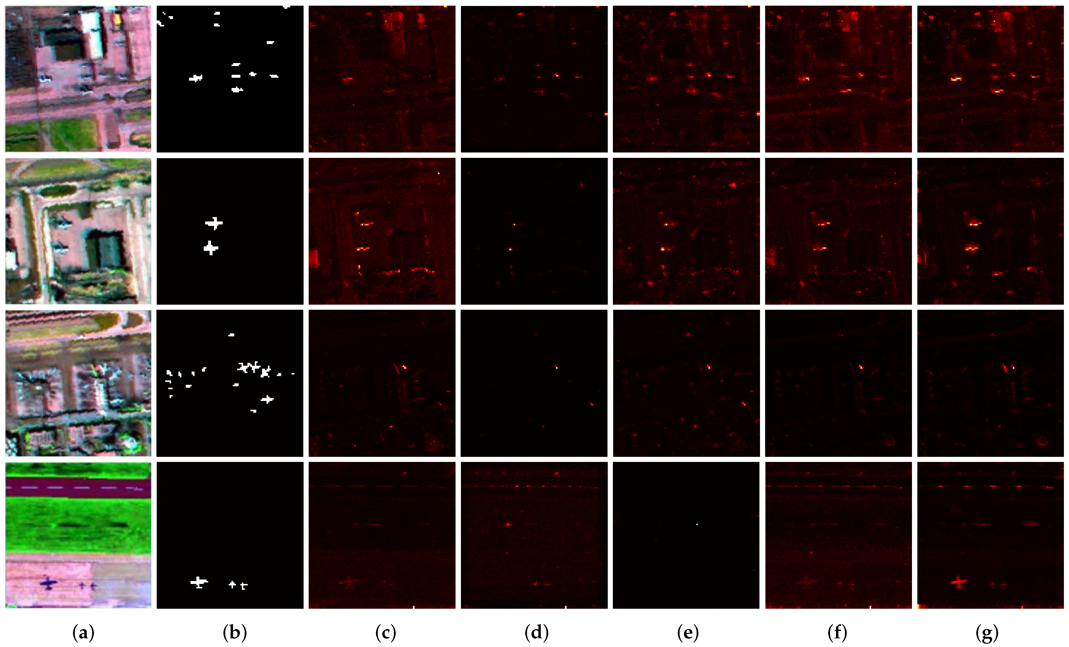
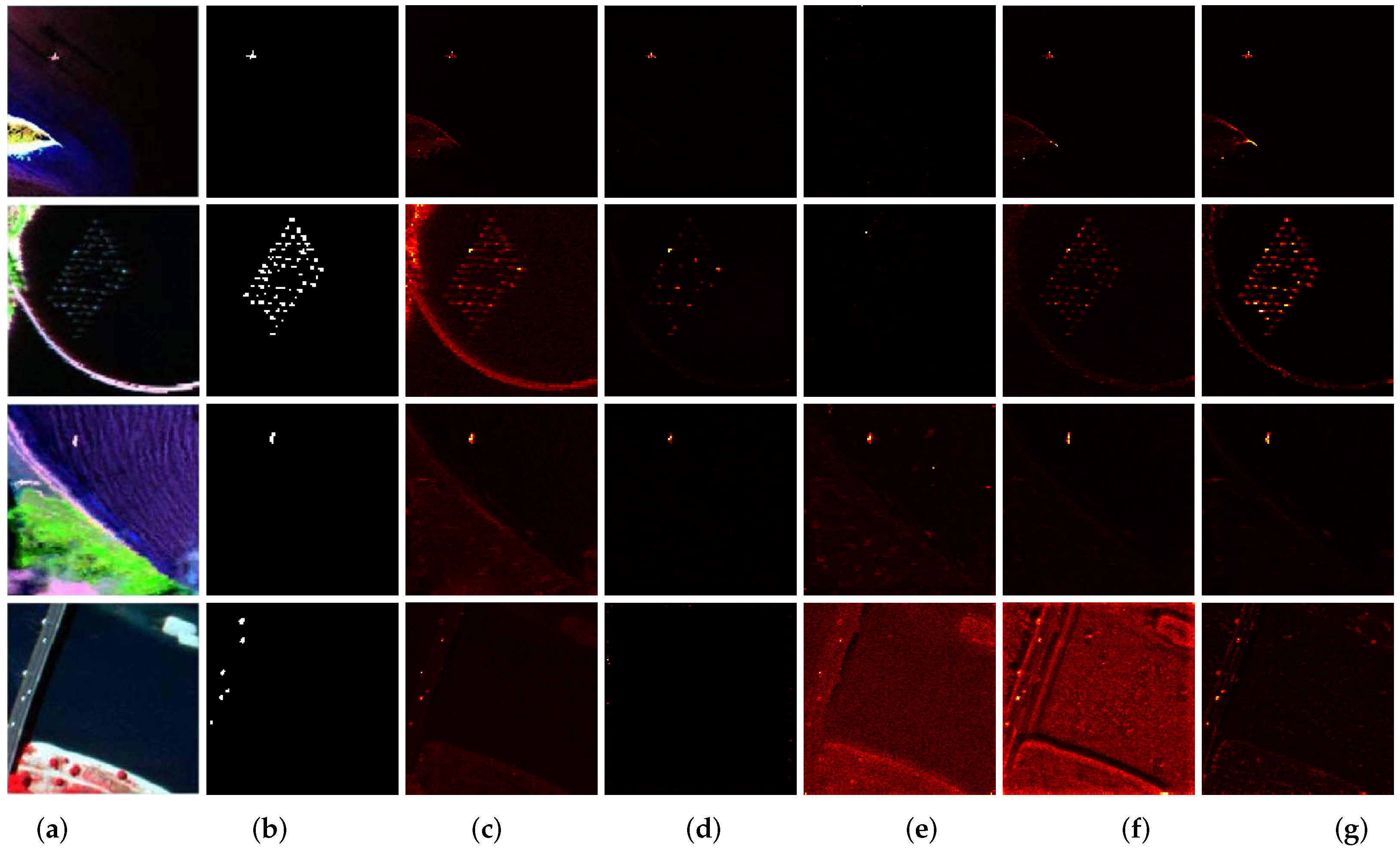
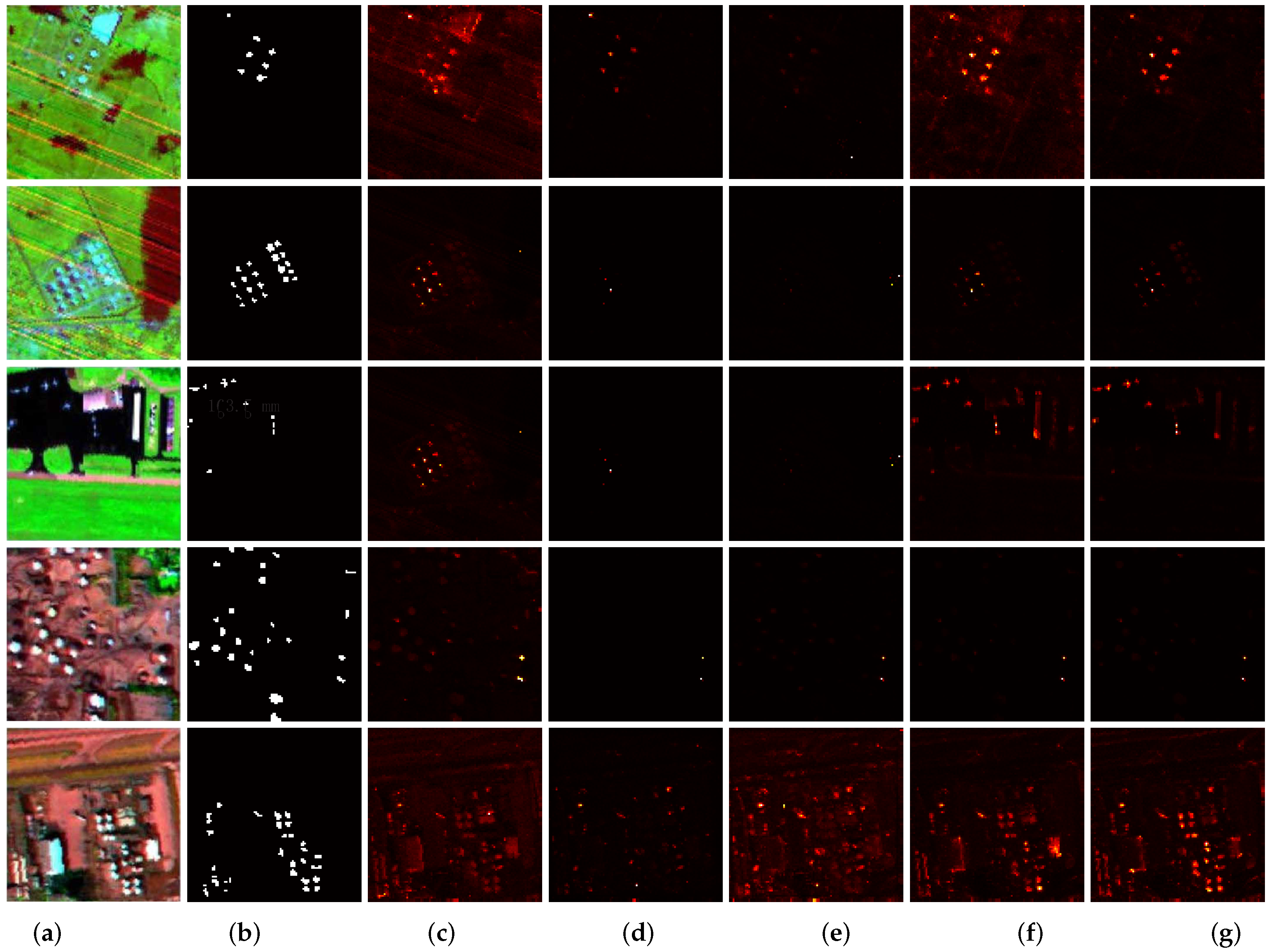
Figure 3, Figure 4 and Figure 5 show the anomaly detection result maps obtained by different methods for three scenarios. As can be seen from Figure 3, the proposed method can detect more pixels in the detection resule. In addition, the SDBP-D and SDBP-S methods can effectively detect most abnormal objects and retain abnormal shapes. Conversely, in the detection result maps obtained by the RX, LRX, and CRD methods, it is difficult to find an abnormal object visually or even detect other objects as abnormal. As shown in Figure 4c, there are many false alarms in the detection results with the RX method. This can indicate that local density information enables further purification of background pixels compared to spectral information. Compared to the SDBP-S method, the SDBP-D improved method usually produces fewer false positives. Taking the Airport scene as an example, the detection result maps obtained by SDBP-D method are obviously clearer than those obtained by the SDBP-S method.
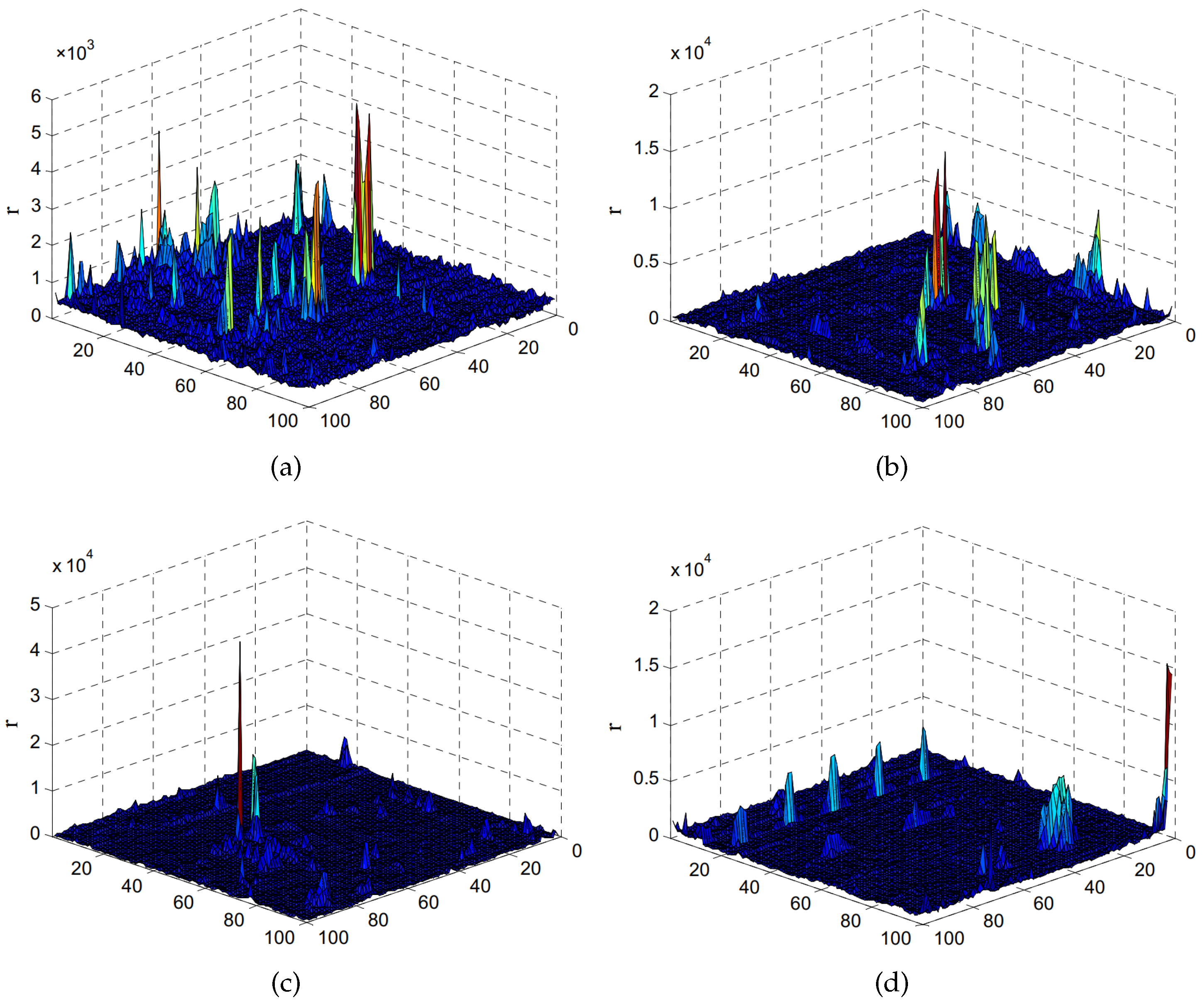
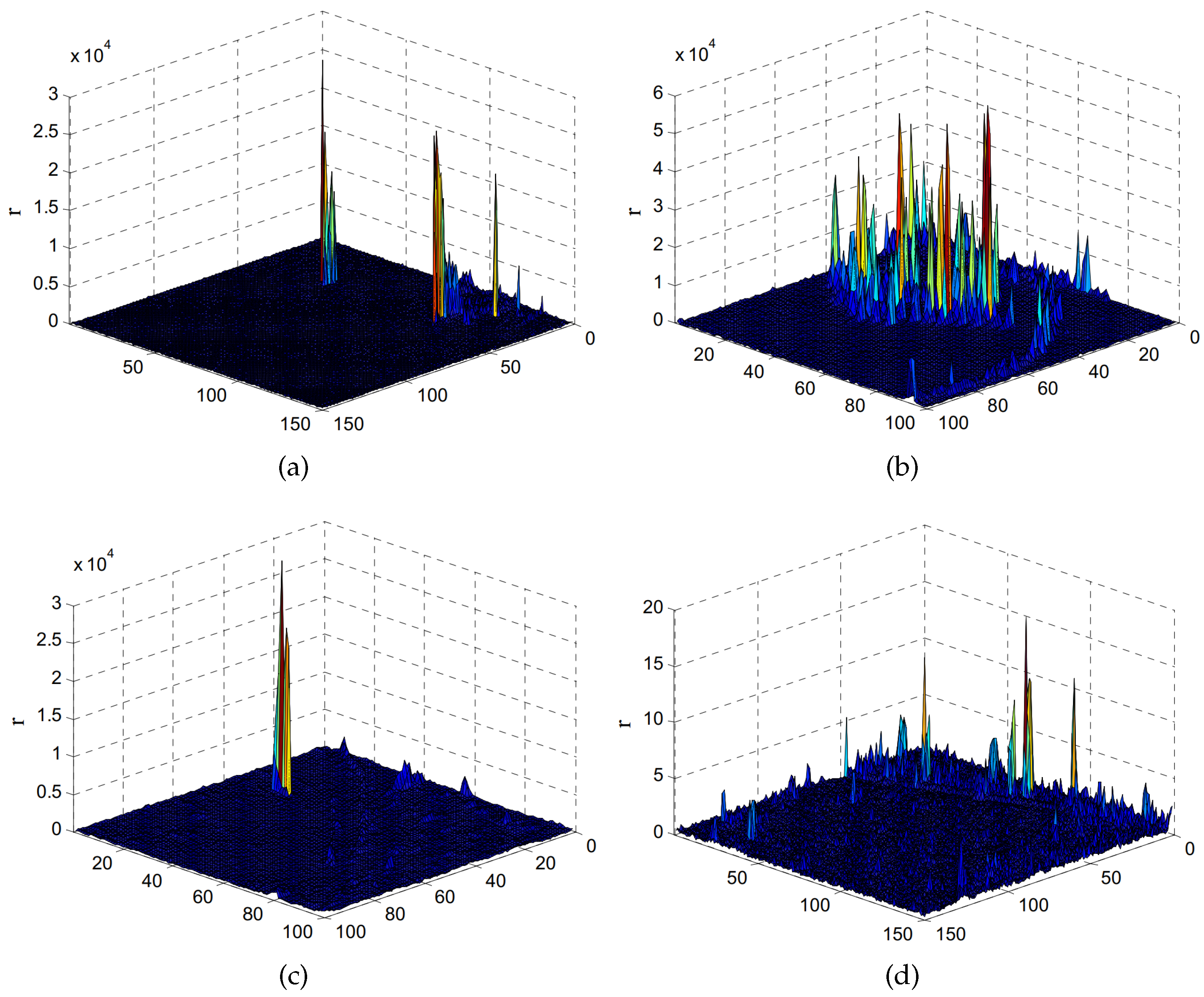
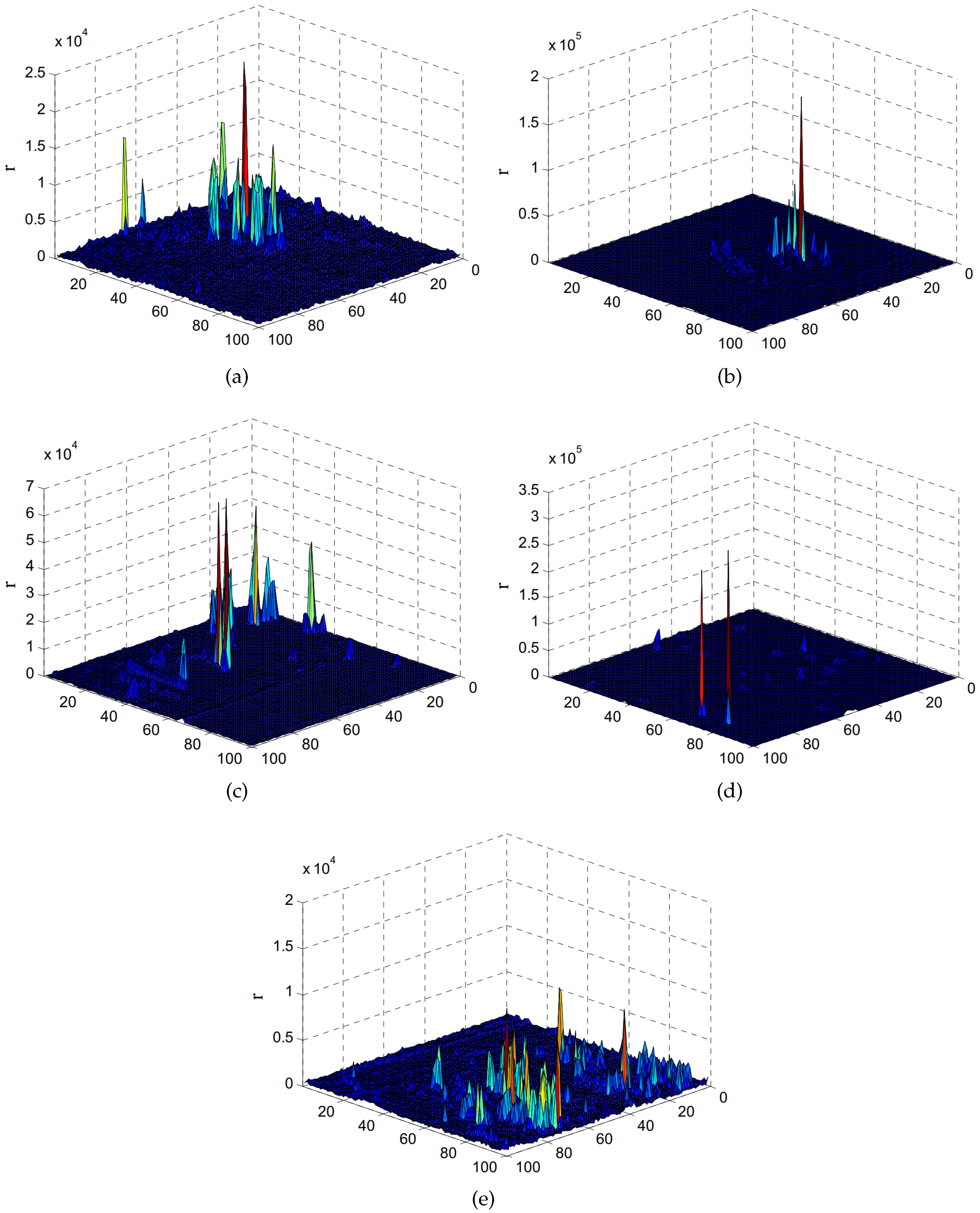
Figure 6, Figure 7 and Figure 8 show the 3D detection results of three scenarios (Airport, Beach, and Urban). The X and Y axes represent the size of the image. The Z-axis represents the Euclidean distance between the center pixel and its approximation. The larger the R value, the more likely the pixel is to be an abnormal pixel. In other words, the pixel with the higher bulge in the 3D detection result is more likely to be an abnormal pixel. For instance, as can be clearly seen in Figure 7, the proposed method can better separate the background and the abnormal target, so that the abnormality is more clear in the detection map.
Figure 9 illustrates the ROC curves obtained for all methods with the Airport-2, Airport-4, Beach-2, and Urban-3 images. As can be seen from the four small figures, the proposed method is superior to the other detection methods. When the false-alarm rate changes from 0.0001 to 1, the detection probabilities of the SDBP-D method are always higher than for other methods. The reason is that the SDBP-D algorithm has a more pure background pixel, which improves detection accuracy. As can be seen from Figure 9a–c, the detection probability curve of the SDBP-D method rises relatively sharply. Figure 9a,b, are the same type of scenes, and their ROC curves change more similarly. In Figure 9d, when the false-alarm rate is low, the detection probability for the SDBP-D method is much higher than for other methods.

4. Discussions

The execute times of SDBP-D anomaly detection method in different scenes are shown in Table 7. From Table 7, we can find that the experiment takes a long time to execute. We can analyze from the following two aspects: On the one hand, the proposed algorithm is based on CRD that is a pixel-level detector and requires a long execution time. on the other hand, the density values in this paper are obtained by calculating the density between pixels and all pixels. On the other hand, the density values calculated in this paper are to calculate all the density between pixels and pixels, which requires calculating the correlation between each pixel and all other pixels in the window. Then, when the density values are cycled in the pixel level detector, the disadvantage of long execution time of the experiment is greatly enlarged. Although the time complexity of this method is a bit high, the method can extract the spatial spectral structure information of HSI and explore the deep spatial relationship between pixels. Experiments on multiple scenes prove that this method effectively improves the detection accuracy.

5. Conclusions

This paper proposes an SDBP method for hyperspectral anomaly detection. The SDBP method uses the local density of pixels instead of directly using spectral information to extract pure background pixels, thus effectively exploring the spatial information of HSI. In addition, it effectively removes most of the abnormal pixels in the background, which makes the background pixels purer, which is more conducive to reducing the false-alarm rate of the detection results. Experiments with several real hyperspectral datasets captured from different scenes demonstrate that the proposed SDBP method is superior to other methods at measuring the quantity and visual quality of detection maps. However, the proposed method may detect two targets as one during the detection process and is not computationally efficient compared with other latest methods. Therefore, multi-task learning should be integrated into the SDBP method in future work to further improve the detection performance. Moreover, designing a more effective technique for SDBP of hyperspectral anomaly detection will be the research in the future.

Author Contributions

B.T. and N.L. designed the proposed model and implemented the experiments. N.L. and Z.L. drafted the manuscript. G.Z. contributed to the improvement of tho proposed model and edited the manuscript. B.T. and X.O. provided overall guidance to the project, reviewed and edited the manuscript and obtained funding to support this research.

Funding

This work was supported in part by the National Natural Science Foundation f China under Grant 61977022 and 51704115, by the Natural Science Foundation of Hunan Province under Grant 2019JJ50212, 2019JJ50211, 2017JJ2107 and 2018JJ2155, by the Hunan Provincial Innovation Foundation for Postgraduate under Grant CX2018B771 and CX20190914, by the Hunan Emergency Communication Engineering Technology Research Center under Grant 2018TP2022, by the Engineering Research Center on 3D Reconstruction and Intelligent Application Technology of Hunan Province under Grant 2019-430602-73-03-006049, and by Scientific Research Program of Hunan Province Education Department under Grant 17C0174.

Acknowledgments

Thanks for the funding support.

Conflicts of Interest

The authors declare no conflict of interest.

References

  1. Stein, D.W.; Beaven, S.G.; Hoff, L.E.; Winter, E.M.; Schaum, A.P.; Stocker, A.D. Anomaly Detection from Hyperspectral Imagery. IEEE Signal Process. Mag. 2002, 19, 58–69. [Google Scholar] [CrossRef]
  2. Borengasser, M.; Hungate, W.S.; Watkins, R. Hyperspectral Remote Sensing: Principles and Application. Iasri 2007, 31, 1249–1259. [Google Scholar]
  3. Xu, Y.; Wu, Z.; Chanussot, J.; Wei, Z. Nonlocal Patch Tensor Sparse Representation for Hyperspectral Image Super-Resolution. IEEE Trans. Image Process. 2019, 28, 3034–3047. [Google Scholar] [CrossRef] [PubMed]
  4. Berger, K.; Atzberger, C.; Danner, M.; D’Urso, G.; Mauser, W.; Vuolo, F.; Hank, T. Evaluation of the PROSAIL Model Capabilities for Future Hyperspectral Model Environments: A Review Study. Remote Sens. 2018, 10, 85. [Google Scholar] [CrossRef]
  5. Pelta, R.; Ben-Dor, E. Assessing the Detection Limit of Petroleum Hydrocarbon in Soils using Hyperspectral Remote-sensing. Remote Sens. Environ. 2019, 224, 145–153. [Google Scholar] [CrossRef]
  6. Justice, C.O.; Vermote, E.; Townshend, J.R.; Defries, R.; Roy, D.P.; Hall, D.K.; Salomonson, V.V.; Privette, J.L.; Riggs, G.; Strahler, A.; et al. The Moderate Resolution Imaging Spectraoradiometer (MODIS): Land Remote Sensing for Global Change Research. IEEE Trans. Geosci. Remote Sens. 1998, 36, 1228–1249. [Google Scholar] [CrossRef]
  7. Hong, D.; Yokoya, N.; Chanussot, J.; Zhu, X. An Augmented Linear Mixing Model to Address Spectral Variability for Hyperspectral Unmixing. IEEE Trans. Image Process. 2019, 28, 1923–1938. [Google Scholar] [CrossRef] [PubMed]
  8. Xia, J.; Falco, N.; Benediktsson, J.A.; Du, P.; Chanussot, J. Hyperspectral Image Classification with Rotation Random Forest Via KPCA. IEEE J. Sel. Top. Appl. Earth Obs. Remote Sens. 2017, 10, 1601–1609. [Google Scholar] [CrossRef]
  9. Wang, Y.; Fan, M.; Li, J.; Cui, Z. Sparse Weighted Constrained Energy Minimization for Accurate Remote Sensing Image Target Detection. Remote Sens. 2017, 9, 1190. [Google Scholar] [CrossRef]
  10. Zhu, D.; Du, B.; Zhang, L. Target Dictionary Construction-based Sparse Representation Hyperspectral Target Detection Methods. IEEE J. Sel. Top. Appl. Earth Obs. Remote Sens. 2019, 12, 1254–1264. [Google Scholar] [CrossRef]
  11. Chen, F.; Ren, R.; Van de Voorde, T.; Xu, W.; Zhou, G.; Zhou, Y. Fast Automatic Airport Detection in Remote Sensing Images Using Convolutional Neural Networks. Remote Sens. 2018, 10, 443. [Google Scholar] [CrossRef]
  12. Ma, D.; Yuan, Y.; Wang, Q. Hyperspectral Anomaly Detection Based on Separability-Aware Sample Cascade. Remote Sens. 2019, 11, 2537. [Google Scholar] [CrossRef]
  13. Yang, C.; Westbrook, J.; Suh, C.; Martin, D.; Hoffmann, W.; Lan, Y.; Fritz, B.; Goolsby, J. An Airborne Multispectral Imaging System Based on Two Consumer-Grade Cameras for Agricultural Remote Sensing. Remote Sens. 2014, 6, 5257–5278. [Google Scholar] [CrossRef] [Green Version]
  14. Waheed, T.; Bonnell, R.B.; Prasher, S.O.; Paulet, E. Measuring performance in precision agriculture: CART—A decision tree approach. Agric. Water Manag. 2006, 84, 173–185. [Google Scholar] [CrossRef]
  15. Salati, S.; van Ruitenbeek, F.; van der Meer, F.; Naimi, B. Detection of Alteration Induced by Onshore Gas Seeps from ASTER and WorldView-2 Data. Remote Sens. 2014, 6, 3188–3209. [Google Scholar] [CrossRef] [Green Version]
  16. Manolakis, D.; Shaw, G.S. Detection Algorithms for Hyperspectral Imaging Applications. IEEE Signal Process. Mag. 2002, 19, 29–43. [Google Scholar] [CrossRef]
  17. Makki, I.; Younes, R.; Francis, C.; Bianchi, T.; Zucchetti, M. A Survey of Landmine Detection using Hyperspectral Imaging. ISPRS J. Photogramm. Remote Sens. 2017, 124, 40–53. [Google Scholar] [CrossRef]
  18. Chen, S.Y.; Lin, C.; Tai, C.H.; Chuang, S.J. Adaptive Window-Based Constrained Energy Minimization for Detection of Newly Grown Tree Leaves. Remote Sens. 2018, 10, 96. [Google Scholar] [CrossRef]
  19. Bioucas-Dias, J.M.; Plaza, A.; Dobigeon, N.; Parente, M.; Du, Q.; Gader, P.; Chanussot, J. Hyperspectral unmixing overview: Geometrical, Statistical, and Sparse Regression-based Approaches. IEEE J. Sel. Top. Appl. Earth Observ. Remote Sens. 2012, 5, 354–379. [Google Scholar] [CrossRef]
  20. Bioucas-Dias, J.M.; Plaza, A.; Camps-Valls, G.; Scheunders, P.; Nasrabadi, N.M.; Chanussot, J. Hyperspectral remote sensing data analysis and future challenges. IEEE Geosci. Remote Sens. Mag. 2013, 1, 6–36. [Google Scholar] [CrossRef]
  21. Zhu, L.; Wen, G. Hyperspectral Anomaly Detection via Background Estimation and Adaptive Weighted Sparse Representation. Remote Sens. 2018, 10, 272–292. [Google Scholar]
  22. Li, W.; Wu, G.; Du, Q. Transferred Deep Learning for Anomaly Detection in Hyperspectral Imagery. IEEE Geosci. Remote Sens. Lett. 2017, 14, 597–601. [Google Scholar] [CrossRef]
  23. Du, B.; Zhao, R.; Zhang, L.; Zhang, L. A Spectral-Spatial based Local Summation Anomaly Detection Method for Hyperspectral Images. Signal Process. 2016, 124, 115–131. [Google Scholar] [CrossRef]
  24. Reed, I.S.; Yu, X. Adaptive multiple-band CFAR Detection of an Optical Pattern with Unknown Spectral Distribution. IEEE Trans. Acoust. Speech Signal Process. 1990, 38, 1760–1770. [Google Scholar] [CrossRef]
  25. Molero, J.M.; Garzón, E.M.; García, I.; Plaza, A. Analysis and Optimizations of Global and Local Versions of the RX Algorithm for Anomaly Detection in Hyperspectral Data. IEEE J. Sel. Top. Appl. Earth Obs. Remote Sens. 2013, 6, 801–814. [Google Scholar] [CrossRef]
  26. Mehmood, A.; Nasrabadi, N.M. Kernel Wavelet-Reed–Xiaoli: An Anomaly Detection for Forward-Looking Infrared Imagery. Appl. Op. 2011, 50, 2744–2751. [Google Scholar] [CrossRef] [PubMed]
  27. Rossi, A.; Acito, N.; Diani, M.; Corsini, G. RX Architectures for Real-time Anomaly Detection in Hyperspectral Images. J. Real-Time Image Process. 2014, 9, 503–517. [Google Scholar] [CrossRef]
  28. Li, M. Anomaly Detection for Hyperspectral Images based on Improved RX Algorithm. In Proceedings of the International Symposium on Multispectral Image Processing and Pattern Recognition, Wuhan, China, 28–29 October 2007; p. 6787. [Google Scholar]
  29. Kwon, H.; Nasrabadi, N.M. Kernel RX-algorithm: A Nonlinear Anomaly Detector for Hyperspectral Imagery. IEEE Trans. Geosci. Remote Sens. 2005, 43, 388–397. [Google Scholar] [CrossRef]
  30. Khazai, S.; Mojaradi, B. A Modified Kernel-RX Algorithm for Anomaly Detection in Hyperspectral Images. Arab. J. Geosci. 2013, 8, 1487–1495. [Google Scholar] [CrossRef]
  31. Plaza, A.J. Anomaly Detection based on a Parallel Kernel RX Algorithm for Multicore Platforms. J. Appl. Remote Sens. 2012, 6, 061503. [Google Scholar]
  32. Zhou, J.; Kwan, C.; Ayhan, B.; Eismann, M.T. A Novel Cluster Kernel RX Algorithm for Anomaly and Change Detection Using Hyperspectral Images. IEEE Trans. Geosci. Remote Sens. 2016, 54, 6497–6504. [Google Scholar] [CrossRef]
  33. Zhao, C.; Li, J.; Meng, M.; Yao, X. A Weighted Spatial-Spectral Kernel RX Algorithm and Efficient Implementation on GPUs. Sensors 2017, 17, 441. [Google Scholar] [CrossRef] [PubMed]
  34. Zhao, C.; Deng, W.; Yan, Y.; Yao, X. Progressive Line Processing of Kernel RX Anomaly Detection Algorithm for Hyperspectral Imagery. Sensors 2017, 17, 1815. [Google Scholar] [CrossRef] [PubMed]
  35. Banerjee, A.; Burlina, P.; Diehl, C. A support vector method for anomaly detection in hyperspectral imagery. IEEE Trans. Geosci. Remote Sens. 2006, 44, 2282–2291. [Google Scholar] [CrossRef]
  36. Zhang, Y.; Du, B.; Zhang, L.; Wang, S. A Low-Rank and Sparse Matrix Decomposition-Based Mahalanobis Distance Method for Hyperspectral Anomaly Detection. IEEE Trans. Geosci. Remote Sens. 2015, 54, 1376–1389. [Google Scholar] [CrossRef]
  37. Hu, Z.; Xiao, M.; Zhang, L.; Liu, S.; Ge, Y. Mahalanobis Distance Based Approach for Anomaly Detection of Analog Filters Using Frequency Features and Parzen Window Density Estimation. J. Electron. Test. 2016, 32, 681–693. [Google Scholar] [CrossRef]
  38. Zhao, C.; Zhang, L.; Cheng, B. A Local Mahalanobis-Distance Method based on Tensor Decomposition for Hyperspectral Anomaly Detection. Geocarto Int. 2019, 34, 490–503. [Google Scholar] [CrossRef]
  39. Zhao, R.; Liu, L.; Junli, L.I. Anomaly Gamma Spectra Detection based on Principal Component Analysis and the Mahalanobis Distance. J. Tsinghua Univ. 2017, 57, 826–831. [Google Scholar]
  40. Du, B.; Zhang, L. A Discriminative Metric Learning Based Anomaly Detection Method. IEEE Trans. Geosci. Remote Sens. 2014, 52, 6844–6857. [Google Scholar]
  41. Zhang, L.L.; Zhao, C.H.; Cheng, B.Z. A Joint Kernel Collaborative-Representation-based Approach for Anomaly Target Detection of Hyperspectral Images. J. Optoelectron. Laser 2015, 26, 2154–2161. [Google Scholar]
  42. Yuan, S.; Zhou, W.; Yuan, Q.; Li, X.; Wu, Q.; Zhao, X.; Wang, J. Kernel Collaborative Representation-Based Automatic Seizure Detection in Intracranial EEG. Int. J. Neural Syst. 2015, 25, 578–1801. [Google Scholar] [CrossRef] [PubMed]
  43. Zaafouri, A.; Sayadi, M.; Fnaiech, F.; al Jarrah, O.; Wei, W. A New Method for Expiration Code Detection and Recognition Using Gabor Features based Collaborative Representation. Adv. Eng. Inf. 2015, 29, 1072–1082. [Google Scholar] [CrossRef]
  44. Li, W.; Du, Q. Collaborative Representation for Hyperspectral Anomaly Detection. IEEE Trans. Geosci. Remote Sens. 2015, 53, 1463–1474. [Google Scholar] [CrossRef]
  45. Tan, K.; Hou, Z.; Wu, F.; Du, Q.; Chen, Y. Anomaly Detection for Hyperspectral Imagery Based on the Regularized Subspace Method and Collaborative Representation. Remote Sens. 2019, 11, 1318. [Google Scholar] [CrossRef]
  46. Su, H.; Wu, Z.; Du, Q.; Du, P. Hyperspectral Anomaly Detection Using Collaborative Representation With Outlier Removal. IEEE J. Sel. Top. Appl. Earth Obs. Remote Sens. 2018, 11, 5029–5038. [Google Scholar] [CrossRef]
  47. Hong-Da, C.; Han-Ye, P.; Bin, W.; Li-Ming, Z. Image Euclidean Distance-based Manifold Dimensionality Reduction Algorithm for Hyperspectral Imagery. J. Infrared Millimeter Waves 2013, 32, 450–455. [Google Scholar]
  48. Lu, T.; Li, S.; Fang, L.; Bruzzone, L.; Benediktsson, J.A. Set-to-setdistance-based Spectral Spatial Classification of Hyperspectral Images. IEEE Trans. Geosci. Remote Sens. 2016, 54, 7122–7134. [Google Scholar] [CrossRef]
  49. Chang, C.-I. An Information-Theoretic Approach to Spectral Variability, Similarity, and Discrimination for Hyperspectral Image Analysis. IEEE Trans. Inf. Theory 2000, 46, 1927–1932. [Google Scholar] [CrossRef]
  50. Liu, J. Quality Assessment of Remote Sensing Image Fusion Using Feature-based Fourth-order Correlation Coefficient. J. Appl. Remote Sens. 2016, 10, 026005. [Google Scholar]
  51. Kang, X.; Zhang, X.; Li, S.; Li, K.; Li, J.; Benediktsson, J.A. Hyperspectral Anomaly Detection With Attribute and Edge-Preserving Filters. IEEE Trans. Geosci. Remote Sens. 2017, 55, 5600–5611. [Google Scholar] [CrossRef]
  52. Rodriguez, A.; Laio, A. Clustering by Fast Search and Find of Density Peaks. Science 2014, 344, 1492–1496. [Google Scholar] [CrossRef] [PubMed]
  53. Ferri, C.; Hernández-Orallo, J.; Flach, P. A Coherent Interpretation of AUC as a Measure of Aggregated Classification Performance. In Proceedings of the 28th International Conference on Machine Learning (ICML-11), Washington, DC, USA, 28 June–2 July 2011; pp. 657–664. [Google Scholar]
Figure 1. Schematic diagram of the proposed method.
Remotesensing 11 02618 g001
Figure 2. Influence of parameter P (The percentage of the highest selected density value) on the SDBP-D method. (a) Airport. (b) Beach. (c) Urban.
Remotesensing 11 02618 g002
Figure 3. Color composites of hyperspectral images (Airport scene) and detection maps of the compared methods. The second column shows the reference detection maps, which are obtained by human labeling. (a) color composites, (b) reference detection maps, (c) RX, (d) LRX, (e) CRD, (f) SDBP-S, (g) SDBP-D.
Remotesensing 11 02618 g003
Figure 4. Color composites of hyperspectral images (Beach scene) and detection maps of the compared methods. The second column shows the reference detection maps, which are obtained by human labeling. (a) color composites, (b) reference detection maps, (c) RX, (d) LRX, (e) CRD, (f) SDBP-S, (g) SDBP-D.
Remotesensing 11 02618 g004
Figure 5. Color composites of hyperspectral images (Urban scene) and detection maps of the compared methods. The second column shows the reference detection maps, which are obtained by human labeling. (a) color composites, (b) reference detection maps, (c) RX, (d) LRX, (e) CRD, (f) SDBP-S, (g) SDBP-D.
Remotesensing 11 02618 g005
Figure 6. Detection result of the proposed SDBP-D method using the Airport dataset. The X and Y axes represent the size of the image. (a) Airport-1. (b) Airport-2. (c) Airport-3. (d) Airport-4.
Remotesensing 11 02618 g006
Figure 7. Detection result of the proposed SDBP-D method using the Beach dataset. The X and Y axes represent the size of the image. (a) Beach-1. (b) Beach-2. (c) Beach-3. (d) Beach-4.
Remotesensing 11 02618 g007
Figure 8. Detection result of the proposed SDBP-D method using the Urban dataset. The X and Y axes represent the size of the image. (a) Urban-1. (b) Urban-2. (c) Urban-3. (d) Urban-4. (d) Urban-5.
Remotesensing 11 02618 g008
Figure 9. ROC evaluation of different anomaly detectors. (a) Airport-2. (b) Airport-4. (c) Beach-2. (d) Urban-3.
Remotesensing 11 02618 g009
Table 1. Some features of the ABU data set.
Airport scene
SceneCapture placeSensorBandResolutionSpectral bandSpectral domain
1Los AngelesAVIRIS2047.1 m400–2500 nmVisible and near-infrared
2Los AngelesAVIRIS2057.1 m400–2500 nmVisible and near-infrared
3Los AngelesAVIRIS2057.1 m400–2500 nmVisible and near-infrared
4GulfportAVIRIS1913.4 m400–2500 nmVisible and near-infrared
Beach scene
SceneCapture placeSensorBandResolutionSpectral bandSpectral domain
1Cat IslandAVIRIS18817.2 m400–2500 nmVisible and near-infrared
2San DiegoAVIRIS1937.5 m400–2500 nmVisible and near-infrared
3Bay ChampagneAVIRIS1884.4 m400–2500 nmVisible and near-infrared
4PaviaROSIS-031021.3 m430–860nmVisible and near-infrared
Urban scene
SceneCapture placeSensorBandResolutionSpectral bandSpectral domain
1Texas CoastAVIRIS20417.2 m400–2500 nmVisible and near-infrared
2Texas CoastAVIRIS20717.2 m400–2500 nmVisible and near-infrared
3GainesvilleAVIRIS1913.5 m400–2500 nmVisible and near-infrared
4Los AngelesAVIRIS2057.1 m400–2500 nmVisible and near-infrared
5Los AngelesAVIRIS2057.1 m400–2500 nmVisible and near-infrared
Table 2. AUC performance of the proposed SDBP-D with varying window size w o u t , w in for the Airport data.
Airport-1Airport-2Airport-3Airport-4
w out w in AUC w out w in AUC w out w in AUC w out w in AUC
3110.954315170.969911170.962617210.9802
3130.956215190.974911190.965817230.9826
3150.952915210.973313150.956517250.9827
5110.953117190.979913170.966119230.9836
5130.955717210.974613190.966219250.9831
5150.953919210.974615170.957221250.9818
Table 3. AUC performance of the proposed SDBP-D with varying window size w o u t , w in for the Beach data.
Beach-1Beach-2Beach-3Beach-4
w out w in AUC w out w in AUC w out w in AUC w out w in AUC
350.9955350.98663130.9998350.9611
3130.9925370.98293150.9999370.9514
590.9949390.96993170.9998390.9499
5110.9959570.97365130.9998570.9696
5130.9919590.96185150.9998590.9579
7110.9912790.94935170.9998790.9667
Table 4. AUC performance of the proposed SDBP-D with varying window size w o u t , w in for the Urban data.
Urban-1Urban-2Urban-3Urban-4Urban-5
w out w in AUC w out w in AUC w out w in AUC w out w in AUC w out w in AUC
390.998513170.99693130.99463150.9969390.9871
3110.998913190.99833150.99483170.99723110.9877
3130.998813210.96893170.99453190.99713130.9868
590.998715170.99625130.99405150.9967590.9866
5110.998915190.99845150.99445170.99665110.9868
5130.998815210.97525170.99325190.99665130.9856
Table 5. Parameters of Airport-Beach-urban (ABU) datasets in SDBP-D anomaly detection method.
Airport SceneBeach SceneUrban Scene
Images w out w in PImages w out w in PImages w out w in P
Airport-11330.9Beach-11150.8Urban-11150.8
Airport-219171Beach-2530.6Urban-219150.8
Airport-317130.8Beach-31530.8Urban-31530.8
Airport-423191Beach-4750.5Urban-41730.8
Urban-51130.7
Table 6. AUC scores on the Airport-Beach-Urban (ABU) dataset in the SDBP-D, SDBP-S, RX, LRX, and CRD anomaly detection methods.
Airport Scene
ImagesSDBP-DSDBP-SRXLRXCRD
Airport-10.96150.96430.82260.96630.9607
Airport-20.98420.95170.84060.94910.9207
Airport-30.96620.96400.92890.93460.9472
Airport-40.99300.98310.95210.88730.8217
Average0.97620.96580.88610.93430.9126
Beach Scene
ImagesSDBP-DSDBP-SRXLRXCRD
Beach-10.99590.99490.98280.99770.9672
Beach-20.98760.97090.91060.97530.9221
Beach-30.99990.99990.99980.99970.9991
Beach-40.97630.94930.95330.95200.9009
Average0.98990.97870.96170.98130.9474
Urban Scene
ImagesSDBP-DSDBP-SRXLRXCRD
Urban-10.99890.99750.99060.99670.9927
Urban-20.99840.99680.99460.90230.9304
Urban-30.99460.99230.95120.96030.9397
Urban-40.99720.99560.98870.91910.9516
Urban-50.98770.97790.96930.93210.9305
Average0.99540.99200.97880.94210.9489
Table 7. The average execution time (seconds) of the different methods in all scenes of the ABU dataset.
AirportBeachUrban
MethodAUCTimeMethodAUCTimeMethodAUCTime
RX0.88610.1608RX0.96170.2655RX0.97880.3533
LRX0.934351.69LRX0.981359.73LRX0.942157.59
CRD0.912670.67CRD0.9474108.63CRD0.948969.66
SDBP-S0.965811846.93SDBP-S0.97872824.12SDBP-S0.992015121.68
SDBP-D0.97622098.80SDBP-D0.98992889.40SDBP-D0.99547637.45