Article

Reconstructing One Kilometre Resolution Daily Clear-Sky LST for China’s Landmass Using the BME Method

1
State Key Laboratory of Remote Sensing Science, Faculty of Geographical Science, Beijing Normal University, Beijing 100875, China
2
Beijing Key Laboratory of Environmental Remote Sensing and Digital City, Beijing Normal University, Beijing 100875, China
*
Author to whom correspondence should be addressed.
Remote Sens. 2019, 11(22), 2610; https://doi.org/10.3390/rs11222610
Submission received: 18 September 2019 / Revised: 4 November 2019 / Accepted: 5 November 2019 / Published: 7 November 2019
(This article belongs to the Special Issue Remote Sensing Monitoring of Land Surface Temperature (LST))

Abstract

:
The land surface temperature (LST) is a key parameter used to characterize the interaction between land and the atmosphere. Therefore, obtaining highly accurate, spatially consistent and temporally continuous LSTs in large areas is the basis of many studies. The Moderate Resolution Imaging Spectroradiometer (MODIS) LST product is commonly used to achieve this. However, it has many missing values caused by clouds and other factors. The current gap-filling methods need to be improved when applied to large areas. In this study, we used the Bayesian maximum entropy (BME) method, which considers spatial and temporal correlation, and takes multiple regression results of the Normalized Difference Vegetation Index (NDVI), Digital Elevation Model (DEM), longitude and latitude as soft data to reconstruct space-complete daily clear-sky LSTs with a 1 km resolution for China’s landmass in 2015. The average Root Mean Square Error (RMSE) of this method was 1.6 K for the daytime and 1.2 K for the nighttime when we simultaneously covered more than 10,000 verification points, including blocks that were continuous in space, and the average RMSE of a single discrete verification point for 365 days was 0.4 K for the daytime and 0.3 K for the nighttime when we covered four discrete points. Urban and snow land cover types have a higher accuracy than forests and grasslands, and the accuracy is higher in winter than in summer. The high accuracy and great ability of this method to capture extreme values in urban areas can help improve urban heat island research. This method can also be extended to other study areas, other time periods, and the estimation of other geographical attribute values. How to effectively convert clear-sky LST into real LST requires further research.

Graphical Abstract

1. Introduction

The land surface temperature (LST), generally defined as the radiative skin temperature of the ground, is closely related to the radiative budget and energy fluxes between the atmosphere and the ground [1,2,3,4]. LST plays an important role in the estimation of climate models, environmental models and evapotranspiration models, as well as the calculation of drought indices, soil moisture contents and mortality rates [5,6,7,8,9,10,11,12,13,14].
Compared with LST measurements at ground stations, satellite remote sensing observations have the advantages of easy acquisition and complete spatial coverage over large areas. Typical LST products include Advanced Spaceborne Thermal Emission and Reflection Radiometer (ASTER), Moderate Resolution Imaging Spectroradiometer (MODIS) and Meteosat Second Generation Spinning Enhanced Visible and Infrared Imager (MSG-SEVIRI) datasets, with spatial resolutions of 90 m, 1 km and 3 km, respectively [15,16,17]. Among them, the MODIS LST product is the most widely used and best suited for our research because of its appropriate spatial resolution (1 km), high temporal resolution (four overpasses per day), wide coverage (globe), and high retrieval accuracy (approximately better than 1 K). The MODIS instruments were launched on the Sun-synchronous satellites of Terra and Aqua in December 1999 and May 2002, respectively [18]. The MODIS LST products are generated with bands 31 and 32 of MODIS’s 36 spectral using the split window algorithm [2]. The latest version C6 MODIS LST products have different spatial resolutions of 1 km, 6 km, and 0.05° and different temporal resolutions of daily, eight days and monthly. The MOD11A1 and MYD11A1 are 1 km daily Level 3 products in those MODIS LST products. The transit time of Terra corresponding to MOD11A1 is about 10:30 (22:30), while the transit time of Aqua corresponding to MYD11A1 is about 13:30 (1:30). They are both processed into sinusoidal projection and stored in tiles containing 1200 rows and 1200 columns. The quality of MODIS products is continuing to improve, from more than 2 K in the previous versions to less than 2 K (within ±1 K in most cases) in the C6 version [4]. MODIS LST products have been widely used in LST research [19,20,21]. However, the MODIS LST product can only provide usable values under clear-sky conditions, and its spatial integrity is thus affected by clouds or other atmospheric disturbances. Taking China as an example, more than half of the pixels per day have no observations on average, and these gaps seriously hinder the application of the MODIS LST product.
Several gap-filling methods have been developed to reconstruct LSTs under cloudy conditions to obtain spatiotemporally-continuous LST products. In general, these methods can be divided into two main groups: clear-sky LST [19,20,21,22,23,24,25,26,27,28,29,30] and cloudy-sky LST [31,32,33,34,35,36,37] methods. Clear-sky LST represents the retrieved LST assuming no cloud effects, whereas cloudy-sky LST represents the actual LST of the reconstruction considering cloud effects. Usually, clear-sky LST is slightly higher than cloudy-sky LST. The methods for reconstructing cloudy-sky LST, mostly based on surface energy balances, often use passive microwave remote sensing data or require ground station measurements or shortwave radiation products. Nonetheless, microwave data have a coarse spatial resolution and an accuracy that needs improvement. Moreover, ground station measurements or shortwave radiation products with a high spatial and temporal resolution are difficult to obtain. This study focused on reconstructing the clear-sky LST, first, because improving the accuracy of clear-sky LST is conducive to further determining the cloudy-sky LST better, and second, because clear-sky LST can be directly applied to research fields such as numerical weather prediction [38], the identification of diurnal patterns of urban heat islands [39], and calculation of the Temperature-Vegetation Dryness Index (TVDI) or Temperature-Vegetation-soil Moisture Dryness Index (TVMDI) [40,41].
The methods for clear-sky LST may be divided into four categories, according to the underlying principles: considering temporal correlation, considering spatial correlation, considering auxiliary information, and the hybrid method. Details of each category are as follows: (1) LST has a temporal correlation because, for the same pixel at different times, the surface properties are the same and only different weather factors, such as solar radiation and wind speed, cause LST differences. Therefore, the first category reconstructs LST based on the temporal correlation using temporal interpolation methods or methods that employ correlations at different times [22,23]; (2) LST also has a spatial correlation because different pixels at the same time have the same weather factors and different surface properties (such as elevation and land cover), but only the surface properties cause LST differences. The second category thus reconstructs LST based on the spatial correlation using spatial interpolation methods [19,24]; (3) in addition, LST is affected by related factors such as elevation and NDVI. The third category thus estimates the missing LST using the empirical relationship between LST and the auxiliary information, which has a similar spatiotemporal resolution to LST and a better spatial coverage integrity than LST [20,21]; (4) finally, the fourth category is hybrid methods that combine two or three of the above methods, such as spatiotemporal gap-filling methods or spatial interpolation methods that consider auxiliary information [25,26,27,28,29,30]. In general, the hybrid approach is the most promising. Considering only temporal correlation is not suitable for regions with high spatial heterogeneity. If only spatial correlation is taken into account, the results will be inaccurate for areas that have large weather changes in a short period of time. If only auxiliary information is considered, the accuracy of regression and the uncertainty of auxiliary information will affect the final results. In previous studies, there have been relatively few methods suitable for LST reconstruction in large areas. In a region as large as China, where climate change is complex, spatial heterogeneity is high, and auxiliary information has considerable uncertainty, a method is needed that can comprehensively and reasonably consider time correlation, spatial correlation, and auxiliary information, and the uncertainty of auxiliary information should also be considered.
Bayesian maximum entropy (BME) is a spatiotemporal statistical method proposed by Christakos that can provide a systematic and rigorous framework for incorporating hard data, soft data and other sources of information into the estimation of variables [42,43]. BME has several attractive features; it does not need to make any assumptions regarding the linearity of the estimator, the normality of the underlying probability laws, or the homogeneity of the spatial distribution. Moreover, BME is capable of considering uncertainties contained in the data. The method has been successfully applied to numerous areas, such as air pollution, soil properties, water demand and disease [44,45,46,47,48,49,50,51,52,53,54,55,56,57,58,59,60,61]. It has also achieved good results in the gap-filling of remote sensing data [62,63,64]. The BME method is suitable for our research because it can not only take advantage of the temporal correlation and spatial correlation of the LST, but can also explicitly consider the uncertainties of the auxiliary information.
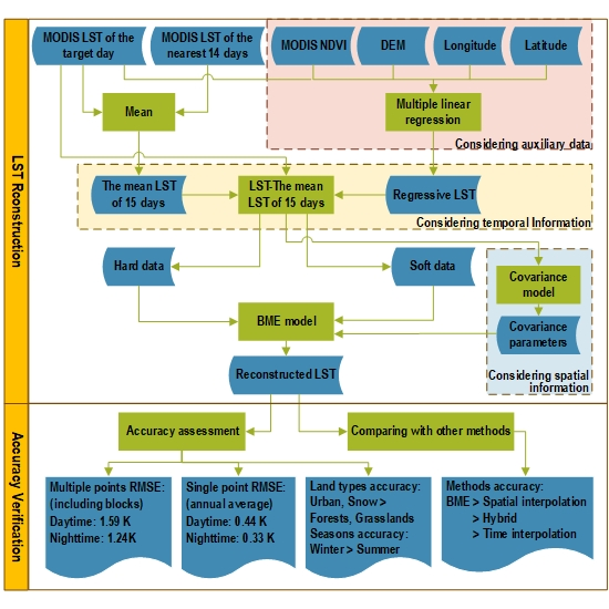
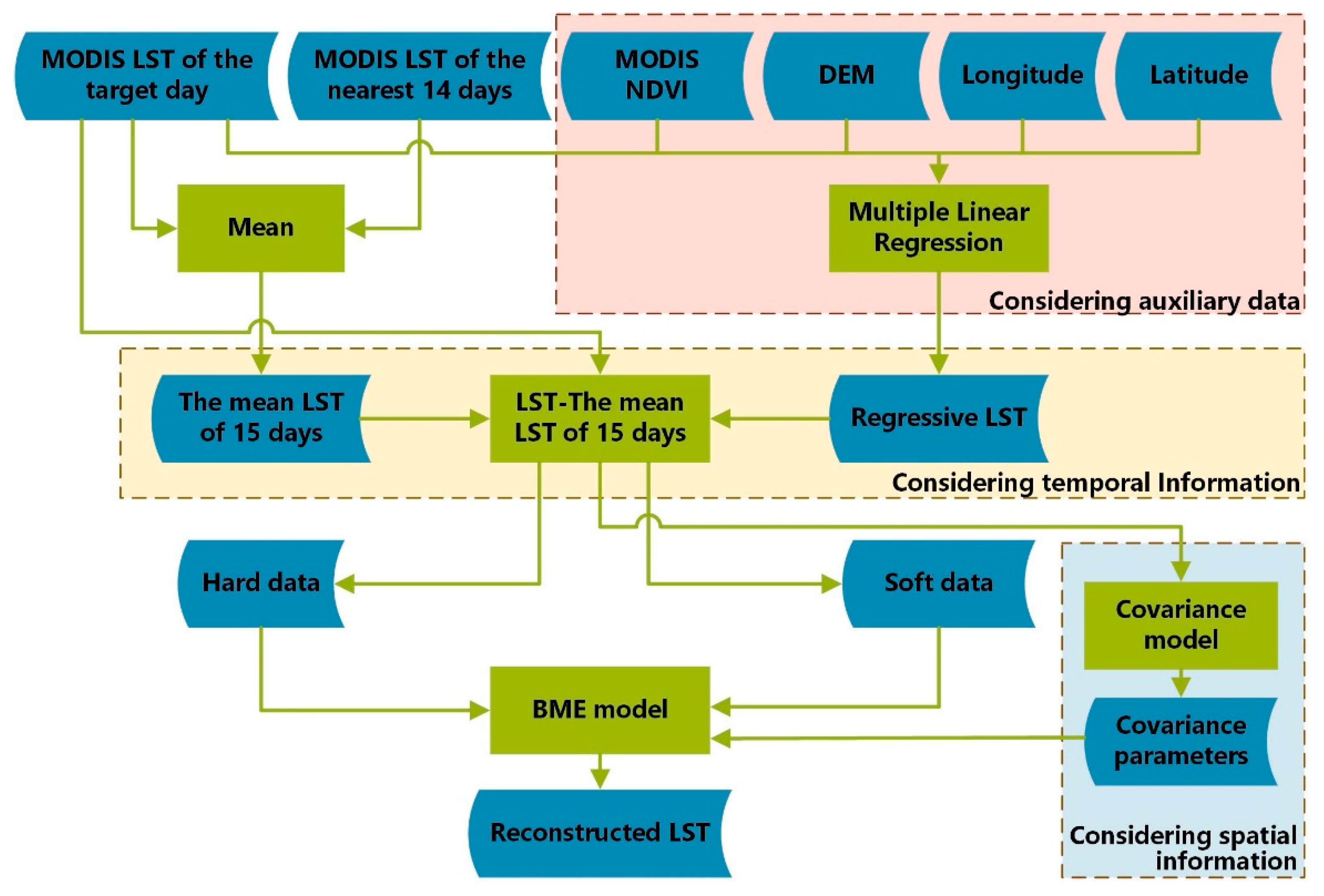
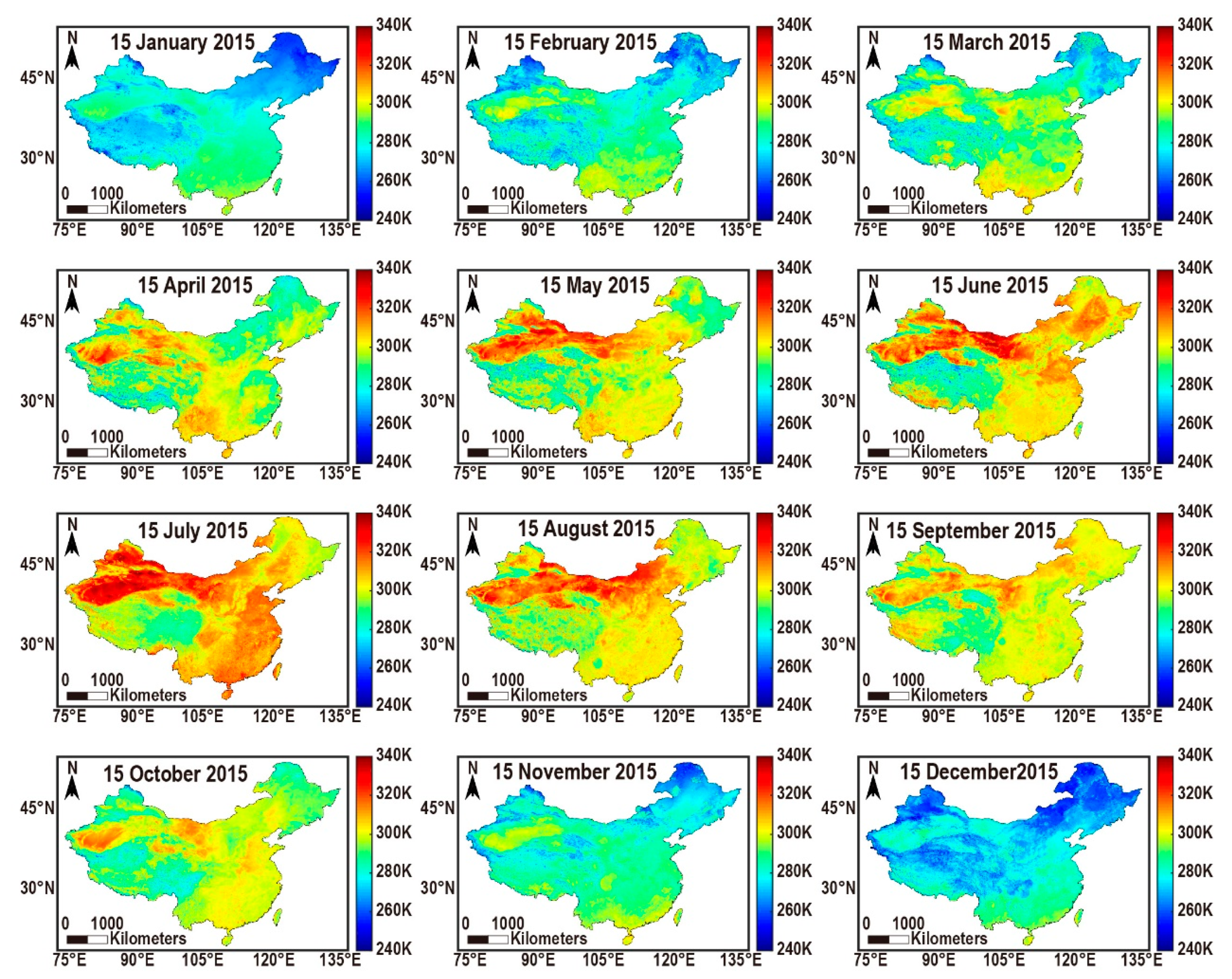
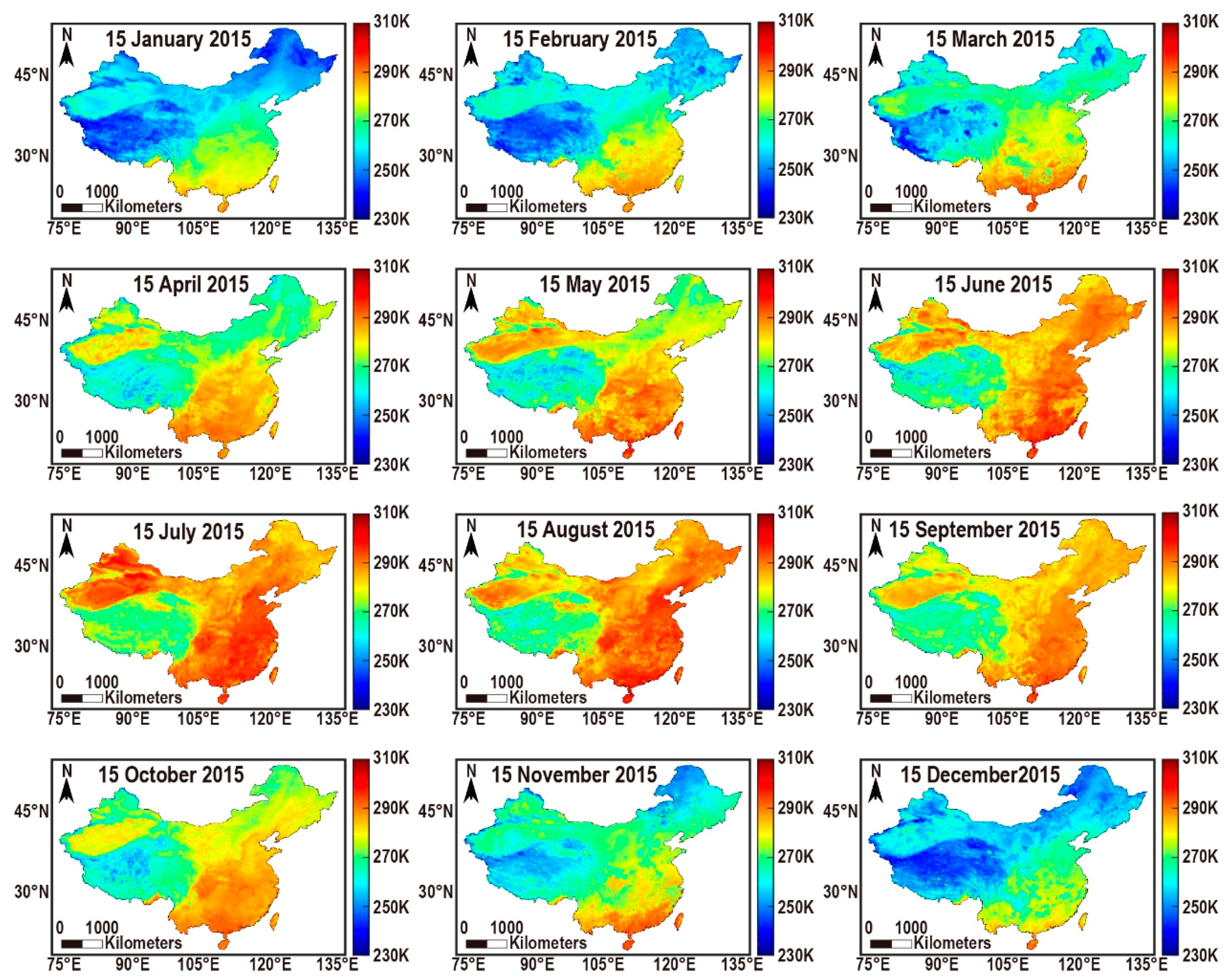
In this study, we applied the BME-based interpolation method to reconstruct 1 km resolution daily clear-sky LST for China’s landmass considering temporal correlation, spatial correlation and auxiliary information. The goals of this article are to (1) examine the feasibility of the BME method to reconstruct LST for the whole of China, (2) discuss the accuracy of the BME method for different land cover types, and (3) compare the BME method with other commonly used LST reconstruction methods.

2. Materials and Methods

2.1. Study Area

In this study, we selected the land area of 34 provinces in China as our study area. China is located on the eastern side of the Eurasian continent and the western shore of the Pacific Ocean; it spans approximately 5500 km from north to south and 5000 km from west to east. The topography across China is complicated and includes plains, plateaus, mountains, hills and basins. It varies from the Qinghai-Tibet Plateau at more than 4000 m above sea level (peaking at 8848 m) to its eastern coastline on the Pacific Ocean. China’s land resources are vast, and its use types are diverse. The cultivated lands are mainly distributed in the eastern region, the forests are distributed in the south and northeast regions, the grasslands are mainly distributed in the central and southwestern regions, and the unused lands are mainly distributed in the northwestern region. China’s climate is governed by monsoonal circulations, and winters with low temperatures and little rain significantly differ from summers with high temperatures and abundant rain [65].

2.2. Data Acquisition and Preprocessing

LST can be affected by many factors [20,66,67]. In view of relatively more critical factors across the Chinese scale and the convenience of data acquisition and processing, NDVI, DEM, longitude and latitude were selected as auxiliary data to regress LST. The following specific datasets were used in this study: (1) For LST, we used the MODIS/Aqua LST Daily L3 Global 1 km SIN Grid product (MYD11A1, Collection 6). LSTs observed throughout the year 2015 were used at local 1:30/13:30 overpass times, which approximate daily minimum and maximum LST values; in the later part of the article, we call them daytime LST and nighttime LST; (2) for NDVI, we selected the MODIS/Aqua 16 day 1 km Vegetation Index product (MYD13A2, Collection6), which has great spatial completeness and the spatial resolution we need. There are 23 NDVI data sets of MYD13A2 for the entire year of 2015; (3) for DEM, we used the Shuttle Radar Topography Mission (SRTM) Digital Elevation Data Version 4 at a 90 m spatial resolution produced to provide consistent, high-quality elevation data. The original DEM data were resized using nearest-neighbours from 90 m to 1 km; (4) for land cover data, we used the MODIS Land Cover Type Yearly Global 500 m product (MCD12Q1) from 2015, which was derived using supervised classifications of MODIS Terra and Aqua reflectance data. We combined all the land types into six categories: forests, grasslands, croplands, barren, urban and snow. Evergreen needleleaf forests, evergreen broadleaf forests, deciduous needleleaf forests, deciduous broadleaf forests, mixed forests, closed shrublands and open shrublands were merged into forests, whilst woody savannas, savannas and grasslands were merged into grasslands. Water was not considered in this study. The pixels were resampled to a 1 km resolution in preparation for the subsequent verification phase; (5) for longitude and latitude, we gave each grid one longitude value and one latitude value at a 1 km spatial resolution based on the WGS84 datum.
MYD11A1, MYD13A2 and MCD12Q1 were provided by the Land Processes Distributed Active Archive Center (LP DAAC) site (https://lpdaac.usgs.gov/). DEM datasets are available from the CGIAR-CSI SRTM 90 m Database site (http://srtm.csi.cgiar.org). In this study, all the above data were downloaded, reprojected, stitched and resized with Google Earth Engine (GEE, https://earthengine.google.com). We processed all the data into 3540 rows × 6166 columns to cover the study area.

2.3. Method

As shown in Figure 1, BME was the core method of this study, and data were prepared for adapting the BME procedure. The three aspects of considering auxiliary data, time correlation, and spatial correlation were used to describe how the three most important input parameters of the BME algorithm, hard data, soft data and covariance models, were constructed. Regarding the auxiliary data, for each image to be estimated, the pixel LSTs with MODIS observations were taken as the dependent variable, and the NDVI image that was taken on the date closest to the estimated image and the elevation, longitude and latitude of the corresponding pixels were taken as independent variables to perform multiple linear regression and obtain the regression coefficients. Then, via the four independent variables of the pixels to be estimated and the respective regression coefficients, the regression LSTs of all the pixels to be estimated were calculated. The regression LSTs were used as the mean value and the mean square error (MSE) between the dependent variable and the predicted value as the variance to construct the Gaussian LST distribution as the soft data. The calculation results of the regression coefficients and the regression R2 of the multiple linear regressions for the daytime and nighttime are shown in Table A1 and Table A2. Regarding time correlation, we subtracted the mean LSTs of 15 days (7 days before and after) from both MODIS observed LSTs used as hard data and regression LSTs used as soft data, and the resulting difference values were input into the BME model as real hard data and soft data, respectively. This is equivalent to the 15 day mean LST minus the LST of the estimated day, which can be understood as the average trend after removing the special weather factors of the day; the LST time correlation could then be taken into account by this simple calculation. After such processing, the LSTs did not need to have trends removed before being input into the BME model, and only the spatial correlation needed to be considered, which could be achieved by the covariance function that represents the spatial dependence. The specific cause analysis can be found in lines 4 to 11 of the fourth paragraph of the introduction. Regarding spatial correlation, we calculated the spatial covariance using the real hard data and soft data mentioned above and input the obtained spatial covariance function name and parameters into the BME model. The relevant parameters of the covariance model calculated in this paper are shown in Table A3 and Table A4.
From the above, it is worth noting that considering the availability of data and the simplicity of method processing, this study made the following assumptions when using the BME method to reconstruct LST: (1) LST changed linearly in a short time (time correlation was considered by subtracting the 15 day mean LST from the LST of the day to be estimated); (2) for the day to be reconstructed, one omnidirectional covariance model of that day can be used in the whole study area; (3) NDVI of each day can be represented by the NDVI data of its adjacent 7 days (the time resolution of the NDVI data was 15 days, so the time interval between the selected NDVI and the estimated image on any day was 0 to 7 days). The main BME conceptual core and framework and the explanations for its use in this research, are shown below.

2.3.1. BME Epistemic Paradigm and Conceptual Core

The BME approach belongs to modern geostatistics, which provide insights into spatiotemporal variables. The epistemic paradigm of BME distinguishes between three main stages of knowledge acquisition, interpretation, and processing, as follows: (1) The prior stage. Spatiotemporal analysis and mapping always starts with a basic set of assumptions and the general knowledge base G. G refers to the background knowledge and the justified beliefs relative to the overall mapping situation; (2) the meta-prior stage. The specific knowledge base S is considered, including hard and soft data. S refers to a particular occurrence or state of affairs at a particular location and at a particular time. Hard data are considered accurate or have a high degree of confidence. Soft data are uncertain observations expressed in terms of interval values, probability statements, empirical charts, and others. That is to say, soft data can have varying levels of uncertainty and may be derived from the direct calculation of the probabilities or the indirect estimation from accumulated experience; (3) the integration or posterior stage. Information from (1) and (2) is processed by means of logical rules to produce the required spatiotemporal map. Therefore, the conceptual core of the BME method is that it aims at informativeness (in terms of prior information relative to the general knowledge G), as well as cogency (in terms of posterior probability relative to the specific knowledge S). BME combines the maximum entropy theory with operational Bayesian statistics to construct its scientific mathematical framework and to implement the above conceptual heart. In general, BME is used to acquire various knowledge bases and to order these bases in an appropriate manner so that, when taken together, they form a realistic picture of the phenomenon of interest.

2.3.2. BME Framework

BME has a rigorous cognitive system and a mathematical reasoning framework. The complete theoretical basis, mathematical formulas and specific derivation processes can be found in reference [43]. The main BME formulas and steps involved in this study are as follows:
f G ( χ k , χ d a t a ) = f G ( χ m a p ) = exp ( α = 1 N μ α ( p m a p ) g α ( χ m a p ) )   d χ m a p exp ( α = 1 N μ α ( p m a p ) g α ( χ m a p ) ) ,
where χ k denotes the LST of the estimated pixel, χ d a t a = ( χ h a r d , χ s o f t ), χ h a r d represents hard data, and χ s o f t represents soft data. In this study, MODIS LST observations were used as hard data and LST Gaussian distributions obtained by multivariate linear regression were used as soft data. The regression process is described above. f G ( χ k , χ d a t a ) denotes the prior pdf of the map χ m a p = ( χ k , χ d a t a ) given the general knowledge base G. μ α ( p m a p ) represents Lagrange multipliers. g α ( χ m a p ) is a set of known functions of χ m a p . In practical applications, prior knowledge usually includes the first-order statistical moment (mean trend) and second-order statistical moment (covariance). The mean trend was not adopted as the first-order statistical moment in this study; rather, the LST difference on the observation day minus the 15 day mean was used. This was done to take time correlation into account and to remove LST instability caused by different weather factors, which resulted in a more stable LST distribution. The second-order statistical moments employed in this study were the spatial covariance functions derived by the difference values calculated above. Such a priori knowledge in this study could consider both the temporal correlation dominated by weather factors and the spatial correlation dominated by surface properties.
f K ( χ k ) = f G ( χ k | χ h a r d , χ s o f t ) = f G ( χ k | χ d a t a ) = f G ( χ k , χ d a t a ) / f G ( χ d a t a )
In Equation (2), f K denotes the posterior pdf of the map χ k , given the total knowledge base K comprised of general knowledge G and specific knowledge S, including hard and soft data. The general knowledge, hard and soft data used in this study were described earlier.
χ k ,   mean =   χ k f K ( χ k ) d χ k
We used the BME mean value ( χ k ,   mean ) as the final estimated LST. The BME mean value could be calculated from the posterior PDF since we sought to penalize large errors more than smaller ones.

2.3.3. BME Implementation

We used the BMElib algorithm package for BME algorithm implementation in MATLAB [68]. The calculation details for each estimated day are as follows. Firstly, the mean value and mean square error of the soft data of each prediction point were input into the probaGaussian.m function of the software package to obtain the soft data information that meets the requirements of the subsequent input. Secondly, the values and position coordinates of hard and soft data were entered into the covario.m and corefit.m functions of the software package to obtain the covariance function name and parameters. Finally, the main function was used to calculate the final result. Information such as hard data, soft data, and covariance was input into the BMEprobaMoments.m function. In addition, the maximum effective distance was set to 15 km, the maximum hard data point was set to 20 points, and the maximum soft data point was set to 3 points.

3. Results

3.1. Spatial Patterns of the Reconstructed LSTs

We selected the 15th day of each month in 2015 to conduct the method experiment and obtained the spatial distribution results of 12 images for both the daytime and nighttime (Figure 2 and Figure 3). In the daytime, an average of 43% of the pixels of the MODIS LST products in the study area had LST observations, and in the nighttime, the value was 51%. That is, there was a missing rate of nearly one-half before filling gaps. The missing LST could be 100% filled using the BME method to generate a complete spatial distribution (Table 1).
In general, the entire study area showed strong spatial heterogeneity that varied in different seasons for both the day and night (Figure 2 and Figure 3).
In winter, the lowest LST for the daytime occurred in northeast China, followed by the Qinghai-Tibet Plateau, whereas the lowest LST for the nighttime appeared in the Qinghai-Tibet Plateau, followed by northeast China. In summer, the lowest LST during the daytime simultaneously occurred in the Qinghai-Tibet Plateau and northeast China, whereas during the nighttime, the LST of the Tibetan Plateau was significantly lower than that in northeast China (Figure 2 and Figure 3). The LST of the Qinghai-Tibet Plateau in southwest China was obviously low due to its high topography, and the LST of northeast China affected by Siberian cold air in winter was also low.
In summer, the highest daytime LST was evident in northwest and central Inner Mongolia, whereas the highest nighttime LST was widely distributed in the south-central and southeastern regions, except for the Qinghai-Tibet Plateau. In winter, the highest daytime LST was distributed in the northwest and southeast regions, but the highest nighttime LST was distributed in the southeast coastal areas (Figure 2 and Figure 3). The LST was usually higher in the northwest and Inner Mongolia due to the large number of deserts. LST was also higher in the southern region because of its low latitude and more solar radiation on the ground.

3.2. Accuracy Assessment

Since the study aimed at clear-sky LST reconstruction, it was not necessary to employ ground observation points for verification. First, this is because clear-sky LST is the theoretical value that is assumed not to be affected by clouds, while the ground observed value is the real value that is affected by clouds, so they cannot be directly compared. Secondly, this is because the acquisition time of the ground station is difficult to coincide with that of MODIS products, and there are also scale effects between points and surfaces. The verification method in this paper is for clear-sky LST. We selected some points with MODIS LST observations to cover them, reconstructed the LST of the covered points with the BME method, and then compared the reconstructed LST values with the known observations of MODIS LST. The verification points must have MODIS LST observations as references for the reconstructed LSTs. Therefore, we selected the points where the MODIS LST observations existed on the 15th of each month in 2015 as the verification points, which also helped to show the accuracy change of points with the same positions over time (Figure 4). There were 10,971 test pixels for the daytime (green points in Figure 4), including 330 forest pixels, 2683 grassland pixels, 537 cropland pixels, 7376 barren pixels, 38 urban pixels and 7 snow and ice pixels. There were 14,376 test pixels for the nighttime (blue points in Figure 4), including 218 forest pixels, 6040 grassland pixels, 425 cropland pixels, 7627 barren pixels, 425 urban pixels and 8 snow and ice pixels. Some of the verification points were spatially continuous and they formed regions of various shapes. The maximum diameter of the regions formed by the verification pixels was close to 60 km, and the estimation accuracy was thus also of reference value for the missing LST values caused by large cloud cover.
The daytime accuracy was mostly lower than that of the nighttime (Figure 5 and Figure 6). The average mean absolute error (MAE) and RMSE values were 1.1 K and 1.6 K, respectively, in the daytime, whereas the values were 0.8 K and 1.2 K in the nighttime, respectively (Figure 7d–f). The accuracy in summer was generally lower than in winter, which decreased and then increased from January to December (Figure 5, Figure 6 and Figure 7d–f). During the daytime, the maximum RMSE was 3.0 K in July and the minimum was 0.8 K in January. During the nighttime, the maximum RMSE was 1.9 K in June and the minimum was 1.0 K in December (Figure 5 and Figure 6). The higher RMSE in summer than in winter may be due to the higher surface heterogeneity in summer than in winter, and the higher RMSE during the day than during the night may be due to more serious cloud cover and more missing values during the day.
In general, the RMSEs of barren land were the largest, with averages of 1.6 K and 1.4 K during the day and night, respectively, whereas the RMSEs of urban areas were the smallest, with averages of 1.0 K and 0.6 K during the day and night, respectively (Figure 7a,b). During the daytime, RMSEs ranked from high to low for barren, grasslands, forests, croplands, urban and snow and ice. During the nighttime, RMSE was in the order of forests, barren, snow and ice, grasslands, croplands and urban (Figure 7c).
As shown in Figure 5 and Figure 6, the changes between day and night of urban LST were the most obvious, and the seasonal changes of ice and snow LST were most obvious. For the daytime, urban LST was close to the average LST of different land cover types, whereas for the nighttime, urban LST was generally higher than the average LST of different land cover types. This indicates that the urban areas have a relatively strong heat island effect at night. The LST of snow and ice was lower in winter and higher in summer.
In addition, we selected one point in Beijing, Wuhan, Shanghai and Guangzhou to estimate the LST for 365 days in 2015 and validated the accuracy with MODIS observations. These four verification points were geographically discrete and located in four major cities of China from north to south (Figure 4). The results are shown in Figure 8. Beijing had fewer than 200 days with LST observations, whereas in the other three cities, the number was less than 100. The maximum number of consecutive missing days was 30 days in Beijing, 40 days in Wuhan, 44 days in Shanghai and 54 days in Guangzhou. BME could fill 100% of the missing LSTs and reconstruct the uninterrupted LST time curve of each pixel for 365 days. As seen from the variation range of the curve, the BME method can describe the change of LST in a relatively fine manner, without smoothing out the maximum and minimum values. The R2 values of the four urban test sites were all greater than 99%, and, except for the RMSE in Wuhan of 0.6 K, the RMSE in the other cities in the day or night was less than 0.5 K. Therefore, the single point test accuracy of the BME method was very high in large cities. The time distribution of LST demonstrated that there were obvious temperature differences between the day and night in the four cities. The four seasons changed most obviously in Beijing because it is located in a typical north temperate semi-humid continental monsoon climate zone, whereas Guangzhou had the smallest difference between the four seasons because of the Marine subtropical monsoon climate.

3.3. Factors that Influence Accuracy

Figure 9 and Figure 10 illustrate the influence of different factors on the LST estimation accuracy represented by RMSE. For the daytime, the Pearson correlation coefficients between the RMSE of the reconstructed LST and the four influencing factors multiple linear regression R2, average LST, ratio of pixels with LST observations to total pixels (namely, completeness) and average NDVI were 0.32, 0.85, −0.21 and 0.86, respectively; for the nighttime, the corresponding Pearson correlation coefficients were 0.22, 0.55, −0.6 and 0.44, respectively. Therefore, the average temperature and average NDVI were strongly correlated with RMSE in the daytime, and the mean LST and completeness were moderately correlated with RMSE in the nighttime. Three rather interesting aspects emerged from the results: (1) The average LST affected the accuracy of the method, where the higher the average temperature, the larger the RMSE; (2) the completeness, or the number of missing pixels, slightly affected the accuracy of the method; (3) the accuracy R2 of multiple linear regression did not affect the accuracy of the method. In this study, R2 varied from 0.39 to 0.90 (from 0.39 to 0.82 during the daytime and from 0.79 to 0.90 during the nighttime). This suggests that the BME method has a great ability to consider the uncertainty of soft data. Since the BME method does not have high requirements for the accuracy of soft data, it can be applied to other large-scale regions, and there is no need to improve the regression accuracy by random forest or other regression methods.

3.4. Comparisons with Other Methods

We compared the BME method with four other commonly used LST gap-filling methods, including Crosson’s method of supplementing MYD data with the same day’s MOD data [22], the time interpolation method HANTS [23], the Kriging spatial interpolation method, and the hybrid gap-filling method proposed by Li [30]. It is worth noting that the same hard data and the same spatial covariance model of the BME method were entered into Kriging, and the only difference was that the Kriging method does not consider soft data. The RMSEs and error distributions of each method are shown in Figure 11. In general, the accuracy of each method ranked from high to low, as follows: BME > Kriging > Hybrid > HANTS > Crosson. It appeared that Crosson’s method had the lowest accuracy, the BME method had the highest accuracy during the daytime, the Kriging method had the highest accuracy during the nighttime, the Hybrid method had a stable accuracy in the day and night, and HANTS had a significantly higher accuracy in the night than in the day.

4. Discussion

4.1. Accuracy Analysis

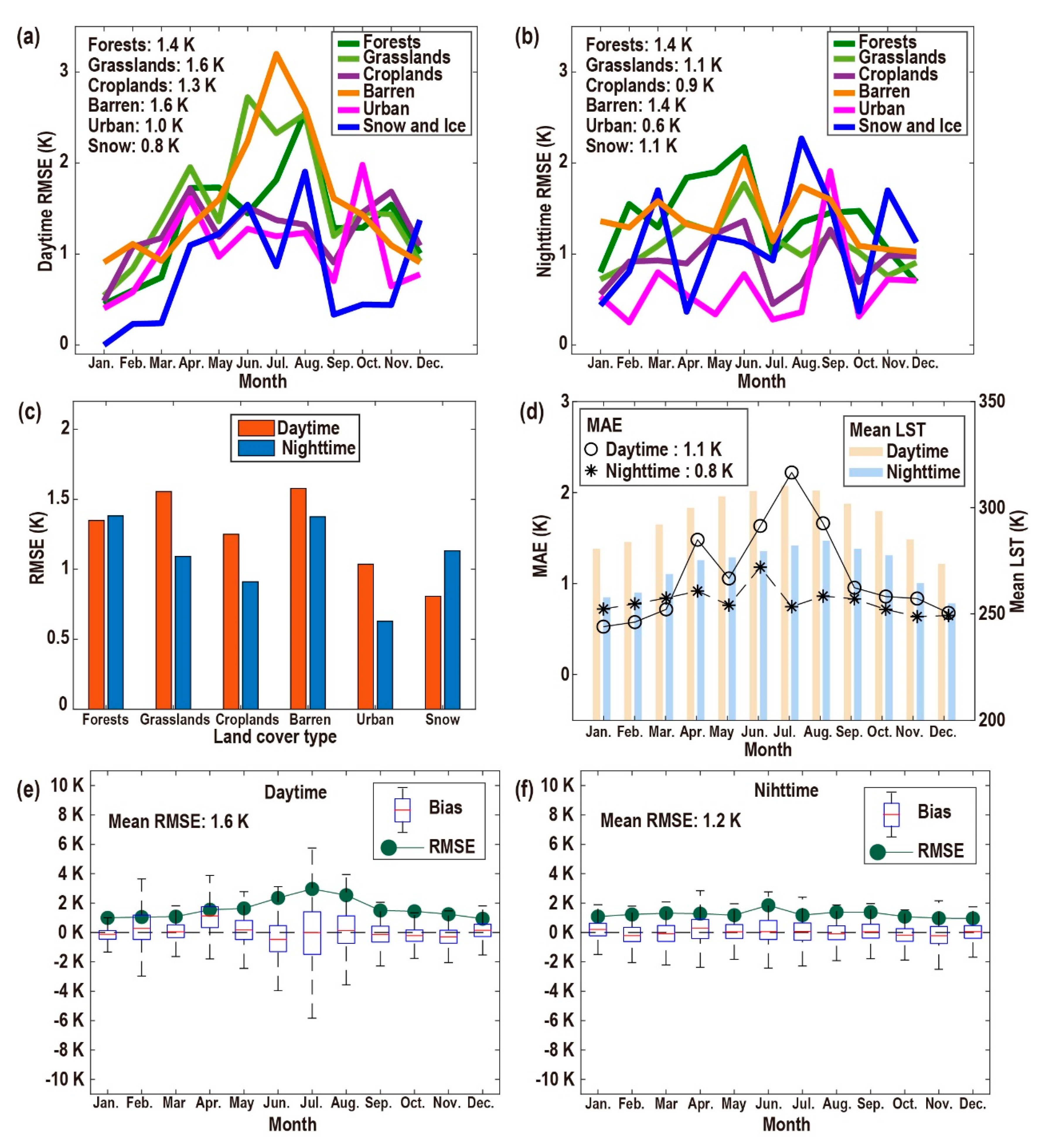
The mean RMSEs in this study were 1.6 K for the daytime and 1.2 K for the nighttime, which were slightly lower than the RMSEs of 3.3 K for the daytime and 2.7 K for the nighttime in Li’s study in a comparably large area [30]. The single point RMSE of approximately 0.5 K is comparable with the RMSE of approximately 2 K under cloud-free conditions in Duan’s study, which selected four ground points for validation [31]. The accuracy of this method is acceptable for large areas with complex geographical and climatic conditions. In addition, this method has a high accuracy in estimating urban LST and can be applied to urban heat island research.
There were different accuracies for different land cover types, which indicates that the accuracy is affected by land cover [34]. The accuracy of barren land and forest was lower than that of urban and cropland because the terrain of barren and forest is more complex, and the spatial heterogeneity is greater. Therefore, the model accuracy can be improved by dividing various terrain regions and then adopting different covariance models for various regions.
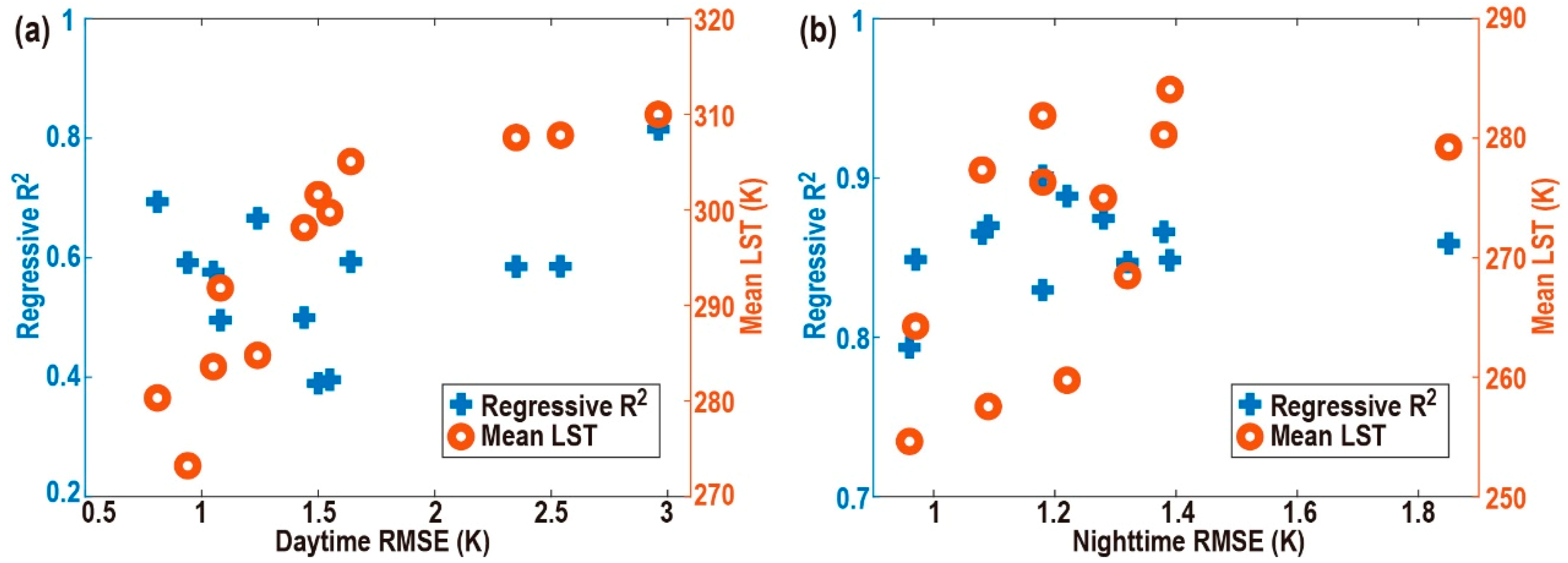
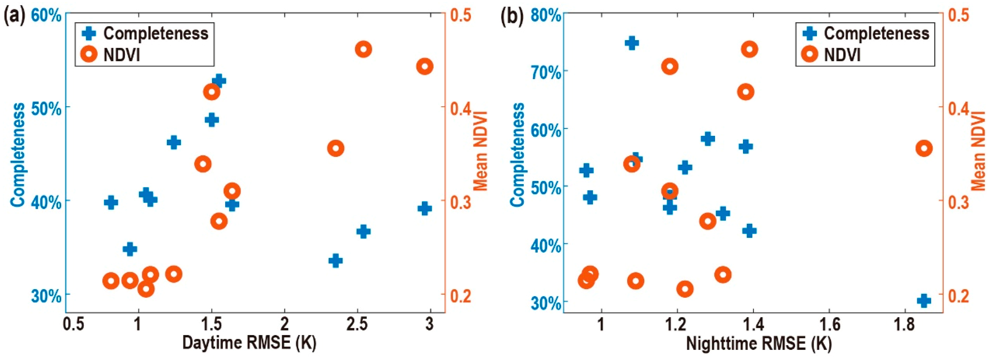
The accuracy decreased with the increase of NDVI and average LST because a high NDVI and high temperature usually represent the summer climate in China, when the cloud cover is large and the distribution is concentrated, which results in large LST gaps. The completeness has only a slight impact on the accuracy, possibly because the accuracy is influenced not only by the number of missing pixels, but also by their maximum diameter and distribution characteristics [69].
When constructing soft data, the accuracy of multiple linear regression does not affect the accuracy; this may be due to the ability of BME to fully consider the uncertainty of soft data. The average regression R2 in this study was nearly 0.6, and in the subsequent application of the BME method to LST reconstruction, when the average regression R2 in the construction process of soft data is greater than 0.6, it is unnecessary to adopt more complex regression methods to improve the regression accuracy.

4.2. Suggestions for Method Selection

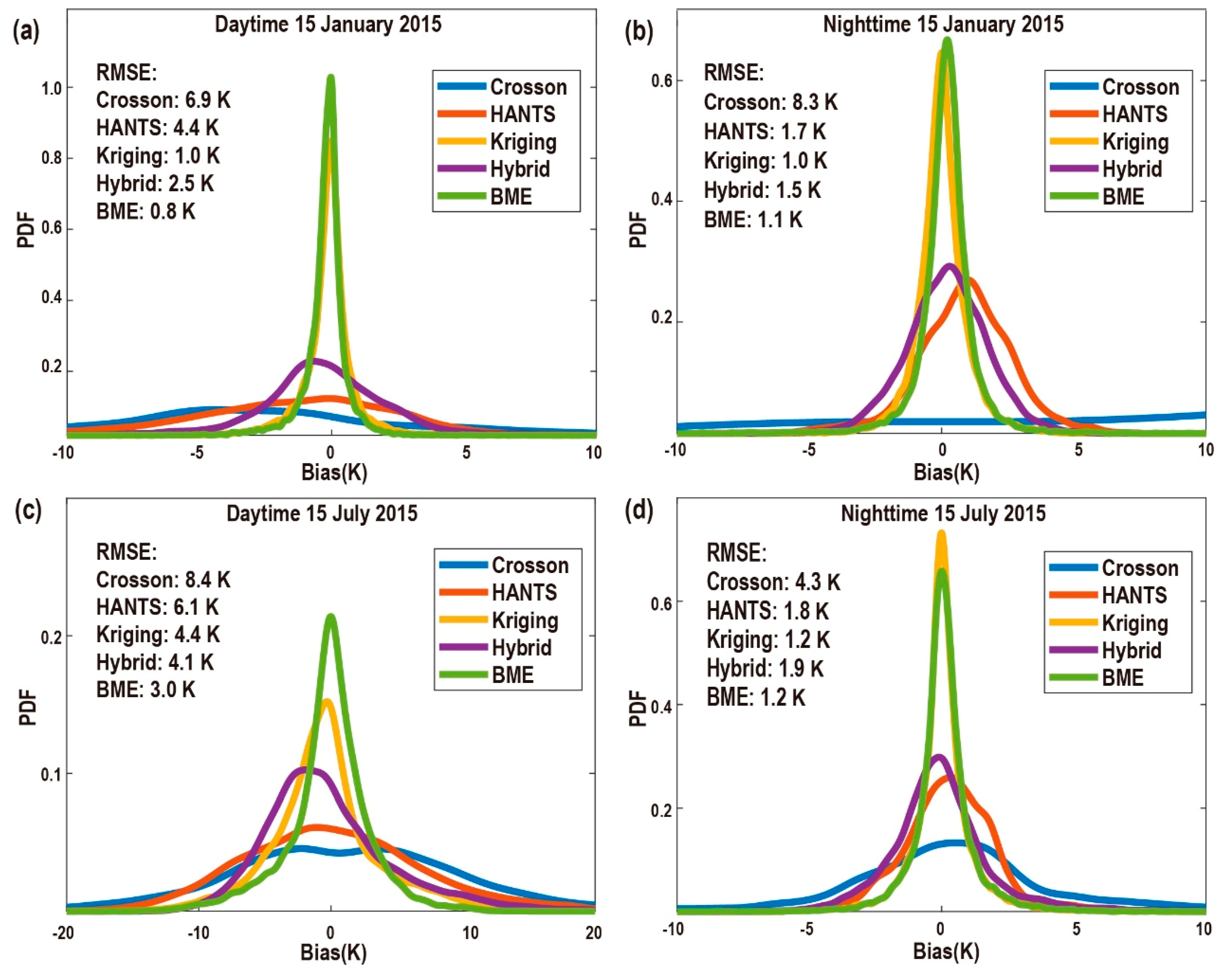
We can learn the characteristics of each LST reconstruction method from Figure 11 and in combination with previous studies. The accuracy of spatial interpolation models is usually higher than that of temporal interpolation models [70]. The time interpolation models have some difficulties in capturing extreme values, and their accuracy is relatively low. Spatiotemporal gap-filling methods are often unable to fill all the missing values at one time, and one usually needs to iterate several times until all the missing values are filled. Spatial interpolation methods, especially the ones that consider auxiliary information, have a high accuracy, but usually take a relatively long time for calculations [25,26]. The study area in this study was large. To balance the calculation time and accuracy, we did not select the spatiotemporal covariance model, but rather the spatial covariance model, to consider the spatial dependence characteristics and the simple 15 day mean value to consider the time dependence characteristics. The spatiotemporal covariance model can be selected in small areas [34,71]. With the development of computing power and multi-core parallelism in the future, the computing speed will become faster.
Suggestions on how to choose an appropriate method to reconstruct LST are as follows: (1) If one hopes for a short computation time and simple computation steps, one can choose the time interpolation method; (2) if a high precision and simple calculation steps are required, the spatial interpolation method is recommended; (3) if one wants to balance the calculation speed and accuracy, we suggest using the spatiotemporal gap-filling method. All of the above three methods can consider introducing auxiliary data to improve the accuracy. In addition, note that the Kriging spatial interpolation method achieved good results in this study area and that Kriging is thus a simple method worth trying. The BME method that we used is a spatial interpolation method that considers auxiliary information, and its precision was very high in this study area.

4.3. Exploration of the Accuracy Improvement

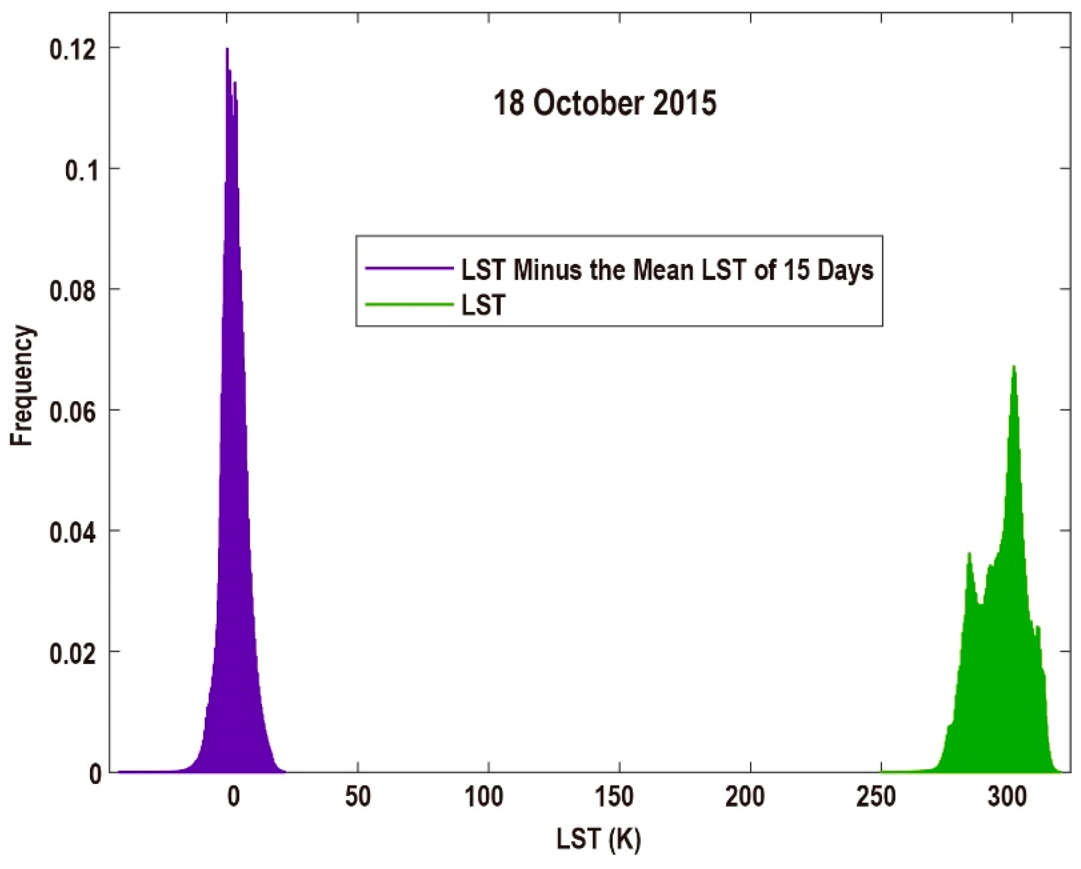
In this part, we will explore methods to improve the accuracy and model applicability based on the assumptions of the method. One assumption of this method was that LST changed linearly in a short time. We thus subtracted the 15 day mean LST from the LST of the constructed day to consider the time correlation. Doing so can also make the data closer to a normal distribution and thus replace the step of trend removal in other BME studies. We selected 18 October, 2015 as an example (there were relatively more MODIS observed LSTs available on that day), as shown in Figure 12. The green part shows that the LST of all pixels on this day presents a non-normal distribution, while the purple part exhibits an approximately normal distribution after subtraction calculation (LST–the mean LST of 15 days) is performed. This operation achieved the desired effect. However, as can be seen from Figure 8, the time variation of LST exhibited both an overall trend and fluctuation. According to the limitation of this study’s assumption, we may improve the accuracy by taking better account of the time correlation. We can do so by introducing the Annual Temperature Cycle (ATC) model, which is a general and smooth curve description of the LST annual change. Considering the time correlation with the LST of the estimated day minus the LST of the corresponding point on the ATC curve, theoretically, will be more accurate than considering the time correlation with the LST of the estimated day minus the LST of the 15 day mean value. We plan to conduct follow-up studies with regards to this.
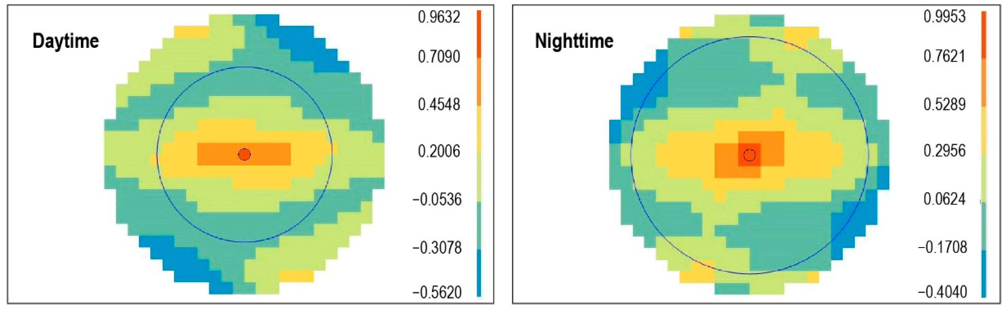
The second assumption of this method was that one omnidirectional covariance model of the constructed day can be used in the whole study area. Here, we want to explore the directivity of the covariance model. We constructed omnidirectional and directional covariance models for 18 October, 2015 (Table 2, Figure 13). As can be seen from the parameters of directional covariance in the study area, the overall characteristic is that the directional covariance is significantly affected by longitude and latitude, and the latitude direction changes faster than the longitude direction.
Omnidirectional and directional covariance models were input into the method in this study to calculate the results, and 10,000 points were randomly selected during the day and night for accuracy verification and comparison. The results show that after considering the directionality of the covariance, the accuracy in the daytime is slightly improved, and the accuracy of the night is not improved (Table 3). It is suggested that directionality can be considered during the daytime in the following research.
In addition, large study areas will have problems with spatial covariance models that differ in different regions. First of all, however, we have not explored how the covariance model changed in different regions of China’s mainland. Moreover, if we want to fill in the LST of the whole study area at once, more detailed regional division may make the model more complicated. How to apply different covariance models in different subregions of the study area is challenging and worthy of further exploration.
The third assumption of this method was that the NDVI of each day can be represented by the NDVI data of its adjacent 7 days. We used 15 day NDVI data because it had values on all pixels to ensure that soft data can be constructed on all LST missing pixels. When the LST was reconstructed on the 15th day of each month in 2015, the nearest NDVI data were selected on 9 January, 10 February, 14 March, 15 April, 17 May, 18 June, 20 July, 21 August, 22 September, 8 October, 8 November and 11 December. There were no results to prove that the closer the reconstruction date was to the obtained date of NDVI, the higher the fitting accuracy and the final LST accuracy were. We believe it was feasible to reconstruct the LST daily with a 15 day NDVI product. Lastly, we cannot accurately calculate the impact of the uncertainty of NDVI datasets on the uncertainty of the final results, which is a limitation of this method.

4.4. Recommendations for Future Studies

Due to the characteristics of the BME method, we cannot accurately determine the uncertainty of the results. At present, we can only obtain the conclusion that at a 1 km spatial resolution, the accuracy of reconstructing the daily LST of China’s landmass with the BME method is acceptable.
For daytime or nighttime LST reconstruction on a certain day, one covariance model can be adopted in the whole research area on that day, which can achieve a reasonable accuracy. If one wants to use this model later, we suggest that it be directly used in the same study area and at the same spatiotemporal resolutions. If other areas or other resolutions are studied, an accuracy analysis should be conducted first to see whether it can meet the actual requirements. The soft data should also be reconstructed according to the geographic and data characteristics of the other study areas. One can try to use the four independent variables in this paper or may introduce other auxiliary data, such as soil moisture and temperature. In the future, we can try to introduce the ATC model, divide different subregions and adopt different covariance models to improve the accuracy of the BME method presented in this study.
When using the BMElib package, it is important to be aware of some parameter settings. The maximum effective distance can be set to a value similar to the range in the covariance model. In order to balance the calculation accuracy and calculation time, we recommend that the maximum number of hard data points should not exceed 50 and the maximum number of soft data points should not exceed 5.
Although clear-sky LST can be applied in some research, the real surface LST is still needed in many fields. This study calculated clear-sky LST, and if one wants to obtain cloudy-sky LST from clear-sky LST, one can refer to Zeng’s method [69]. Adding microwave and ground observation data can also be considered.

5. Conclusions

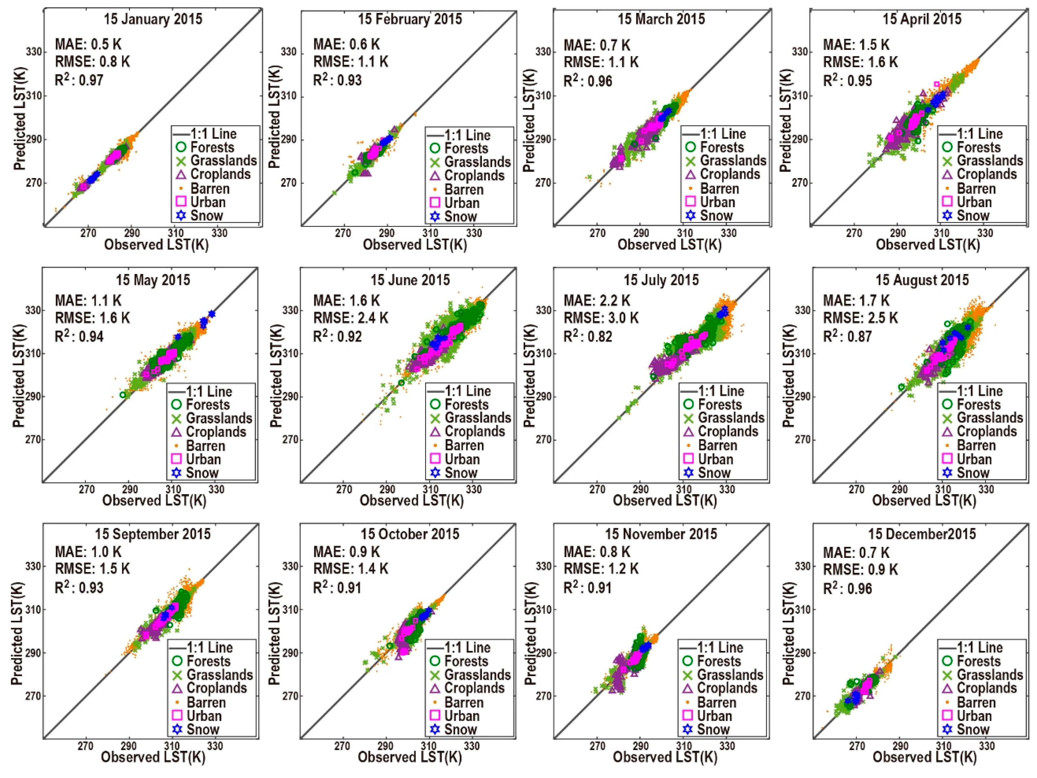
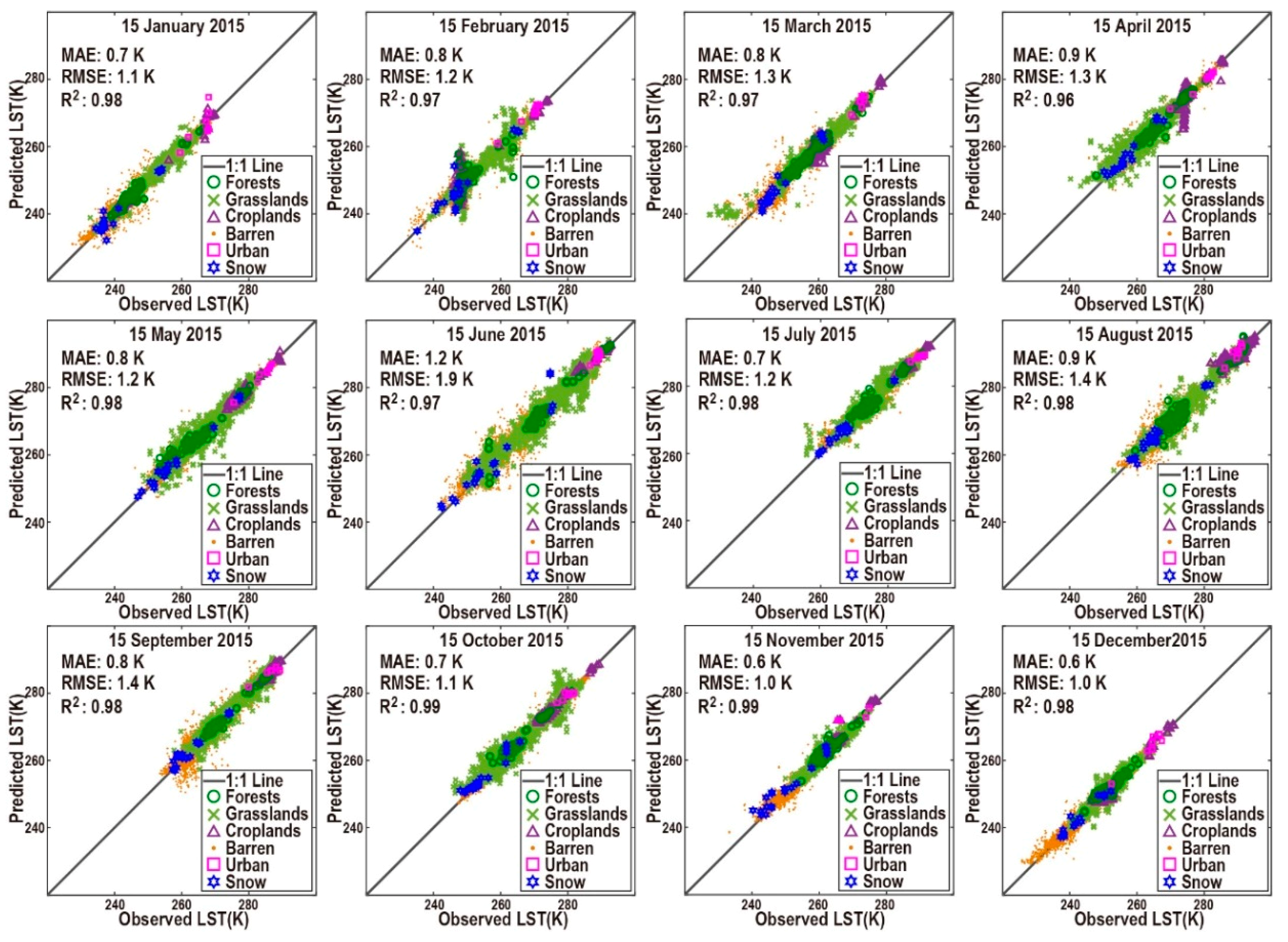
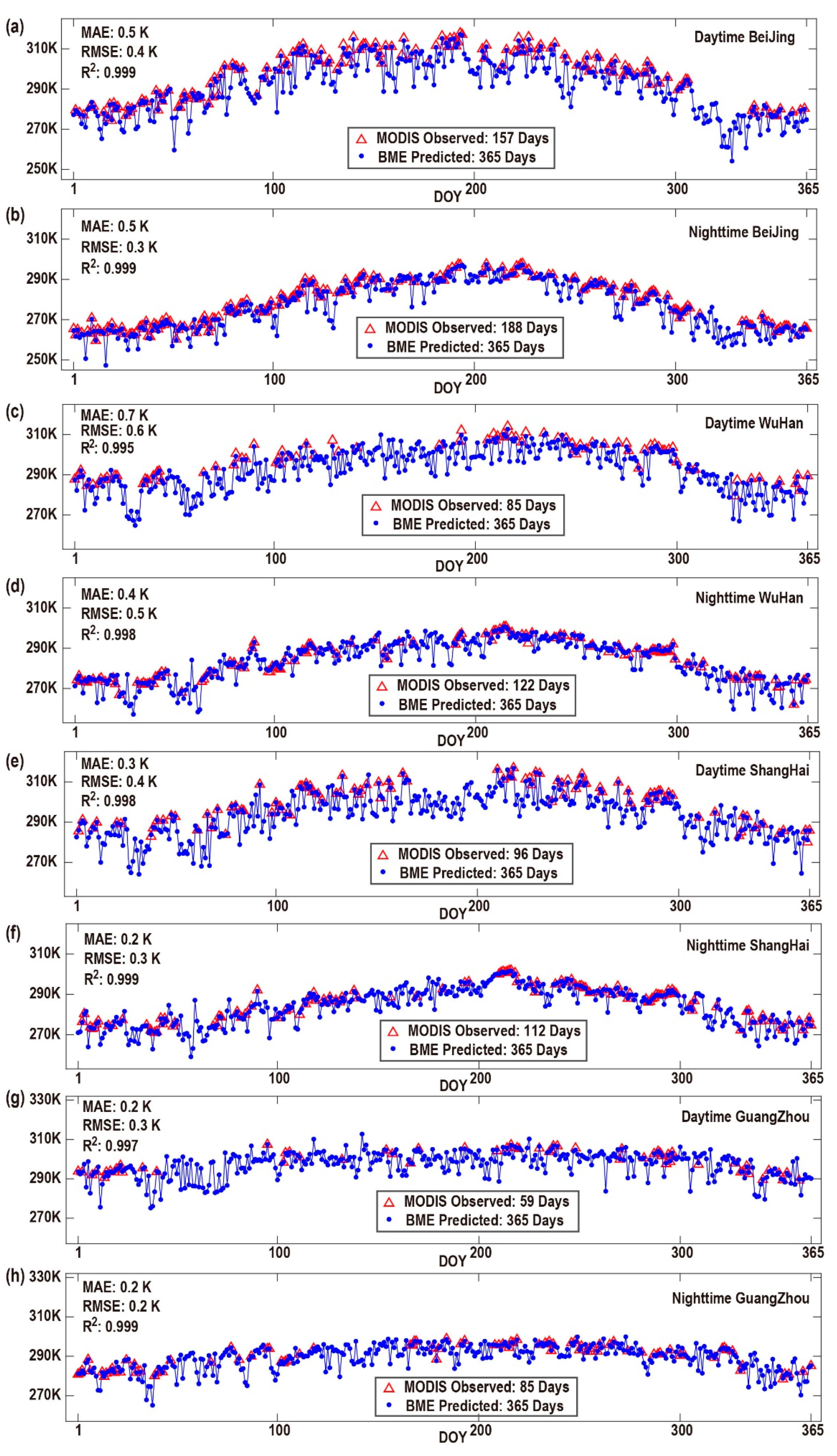
The MODIS LST product has many missing values over wide areas, which hinders its practical application. In this study, we reconstructed the seamless 1 km resolution daily clear-sky LST for China’s landmass based on the BME method, considering spatiotemporal correlation and taking auxiliary data as soft data. The average RMSE was 1.6 K for the daytime and 1.2 K for the nighttime, with the mean absolute error (MAE) of 1.1 K for the daytime and 0.8 K for the nighttime, and the corresponding R2 of 0.92 for the daytime and 0.98 for the nighttime.
This method has the following advantages: (1) It simultaneously considers spatiotemporal correlation and auxiliary data and has a high accuracy in a large area. It has the ability to capture extreme values; (2) the data in this method are easy to obtain and process; (3) simple linear regression is used to construct soft data, and there is no need to adopt more complex regression methods to improve the regression accuracy, as long as the average regression R2 is greater than 0.6; (4) even if the diameter of the missing area is large or the continuous missing time is long, this method does not need multiple step-by-step calculations to gradually fill in the missing pixels, and can estimate all the missing pixels at one time.
There are also some limitations for this method: (1) This method is not applicable when an accuracy of less than 1 K across the entire Chinese landmass is required; (2) when using the method in other study areas and spatiotemporal scales, it is necessary to first consider whether the hypothesis of LST linearity change in a short time and one omnidirectional covariance model can be applied to the entire study area are valid; (3) the method cannot quantitatively calculate the influence of the uncertainty of NDVI and DEM data on the uncertainty of the results; (4) the clear-sky LST should be converted to cloudy-sky LST if the real LST is required.
The results of this study provide a data basis for daily LST analysis and subsequent relevant studies in large areas of China. For the method, its high accuracy and great ability to capture extreme values in urban areas can help improve urban heat island research. It can also be applied to the reconstruction of missing LST values of other years, other regions and other spatial resolutions (such as Landsat), as well as the estimation of missing values of other geographical attributes.

Author Contributions

Conceptualization, Y.Z. and Y.C.; data curation, Y.Z. and Y.L.; formal analysis, Y.Z. and Y.C.; funding acquisition, Y.C. and J.L.; investigation, Y.Z.; methodology, Y.Z.; project administration, Y.C.; software, Y.Z. and Y.L.; supervision, Y.C. and J.L.; validation, Y.Z. and H.X.; visualization, Y.Z.; writing original draft, Y.Z.; writing—review and editing Y.Z., Y.C., Y.L., H.X. and J.L.

Funding

This work was supported by the National Key R&D Program on monitoring, early warning and prevention of major natural disasters under Grant 2017YFC1502406; the Natural Science Foundation of China under Grants 41571342, 41771448 and 51579135; the Beijing Natural Science Foundation under Grant 8192025; and in part by the Beijing Laboratory of Water Resources Security.

Acknowledgments

We are very grateful to Patrick Bogaert (Université Catholique de Louvain; Belgium) and Marc Serre (University of North Carolina at Chapel Hill; USA) for providing us with the MATLAB algorithm package BMElib and to Alexander Kolovos (SpaceTimeWorks, LLC; USA), Hwa-Lung Yu (National Taiwan University, Taipei; Taiwan), Steve Warmerdam and Boris Dev (San Diego State University, CA, USA) for providing us with the MATLAB visualization algorithm package SEKS-GUI. We would also like to thank the Level-1 and Atmosphere Archive & Distribution System (LAADS) Distributed Active Archive Center (DAAC) of NASA for MODIS data and the Consultative Group of International Agricultural Research-Consortium for Spatial Information (CGIAR-CSI) for SRTM DEM data. We would like to thank the anonymous reviewers for their insightful comments and substantial help in improving this article.

Conflicts of Interest

The authors declare no conflict of interest.

Appendix A

Table A1. Regression R2 and regression coefficients of multiple linear regression for the daytime.
DateRegression R2InterceptCoefficient of NDVICoefficient of DEMCoefficient of LatitudeCoefficient of Longitude
15 January, 20150.69366.07−2.10−0.004−1.07−0.39
15 February, 20150.58371.31−5.23−0.004−1.26−0.31
15 March, 20150.50381.25−24.29−0.005−1.52−0.17
15 April, 20150.40369.12−4.05−0.005−0.18−0.50
15 May, 20150.59388.10−26.26−0.007−0.63−0.39
15 June, 20150.59343.54−23.48−0.007−0.10−0.13
15 July, 20150.82373.64−21.95−0.008−0.16−0.35
15 August, 20150.59320.09−28.35−0.005−0.070.10
15 September, 20150.39317.19−14.30−0.003−0.02−0.03
15 October, 20150.50349.92−16.69−0.004−0.52−0.19
15 November, 20150.67370.45−16.05−0.004−1.38−0.21
15 December, 20150.59358.56−8.76−0.003−1.65−0.14
Table A2. Regression R2 and regression coefficients of multiple linear regression for the nighttime.
DateRegression R2InterceptCoefficient of NDVICoefficient of DEMCoefficient of LatitudeCoefficient of Longitude
15 January, 20150.87337.62−18.39−0.005−0.97−0.18
15 February, 20150.89336.19−15.67−0.006−0.98−0.13
15 March, 20150.85330.99−5.02−0.005−1.13−0.06
15 April, 20150.87338.49−9.03−0.005−0.58−0.25
15 May, 20150.83350.82−3.16−0.007−0.66−0.32
15 June, 20150.86300.98−0.42−0.005−0.300.03
15 July, 20150.90326.60−2.70−0.006−0.23−0.21
15 August, 20150.85308.03−2.69−0.005−0.550.07
15 September, 20150.87295.45−2.60−0.004−0.340.07
15 October, 20150.87310.69−2.56−0.005−0.57−0.03
15 November, 20150.85331.74−1.86−0.005−1.25−0.06
15 December, 20150.79324.41−12.13−0.005−0.98−0.09
Table A3. Names and parameters of the spatial covariance model for the daytime.
DateModel NameNuggetPartial SillRange (km)
15 January, 2015exponential0.340.664.03
15 February, 2015exponential0.670.3211.59
15 March, 2015exponential0.380.625.62
15 April, 2015spherical0.500.485.29
15 May, 2015exponential0.400.607.62
15 June, 2015exponential0.570.439.25
15 July, 2015spherical0.690.3110.13
15 August, 2015gaussian0.410.579.78
15 September, 2015spherical0.440.5514.39
15 October, 2015exponential0.320.6813.78
15 November, 2015spherical0.520.4613.28
15 December, 2015exponential0.680.3218.56
Table A4. Names and parameters of the spatial covariance model for the nighttime.
DateModel NameNuggetPartial SillRange (km)
15 January, 2015exponential0.340.666.34
15 February, 2015spherical0.350.6512.08
15 March, 2015spherical0.570.4310.17
15 April, 2015spherical0.560.439.57
15 May, 2015spherical0.390.6117.30
15 June, 2015exponential0.450.553.56
15 July, 2015exponential0.530.4710.54
15 August, 2015gaussian0.310.6710.75
15 September, 2015exponential0.390.619.57
15 October, 2015spherical0.290.7114.79
15 November, 2015exponential0.500.5012.71
15 December, 2015exponential0.300.709.28

References

  1. Norman, J.M.; Becker, F. Terminology in thermal infrared remote sensing of natural surfaces. Agric. For. Meteorol. 1995, 77, 153–166. [Google Scholar] [CrossRef]
  2. Wan, Z.; Dozier, J. A generalized split-window algorithm for retrieving land-surface temperature from space. IEEE Trans. Geosci. Remote Sens. 1996, 34, 892–905. [Google Scholar] [Green Version]
  3. Li, Z.-L.; Tang, B.-H.; Wu, H.; Ren, H.; Yan, G.; Wan, Z.; Trigo, I.F.; Sobrino, J.A. Satellite-derived land surface temperature: Current status and perspectives. Remote Sens. Environ. 2013, 131, 14–37. [Google Scholar] [CrossRef] [Green Version]
  4. Wan, Z. New refinements and validation of the collection-6 MODIS land-surface temperature/emissivity product. Remote Sens. Environ. 2014, 140, 36–45. [Google Scholar] [CrossRef]
  5. Carlson, T.N.; Gillies, R.R.; Schmugge, T.J. An interpretation of methodologies for indirect measurement of soil water content. Agric. For. Meteorol. 1995, 77, 191–205. [Google Scholar] [CrossRef]
  6. Norman, J.M.; Kustas, W.P.; Humes, K.S. Source approach for estimating soil and vegetation energy fluxes in observations of directional radiometric surface temperature. Agric. For. Meteorol. 1995, 77, 263–293. [Google Scholar] [CrossRef]
  7. Zhang, L.; Lemeur, R.; Goutorbe, J.P. A one-layer resistance model for estimating regional evapotranspiration using remote sensing data. Agric. For. Meteorol. 1995, 77, 241–261. [Google Scholar] [CrossRef]
  8. Bodas-Salcedo, A.; Ringer, M.A.; Jones, A. Evaluation of the Surface Radiation Budget in the Atmospheric Component of the Hadley Centre Global Environmental Model (HadGEM1). J. Clim. 2008, 21, 4723–4748. [Google Scholar] [CrossRef]
  9. Kustas, W.; Anderson, M. Advances in thermal infrared remote sensing for land surface modeling. Agric. For. Meteorol. 2009, 149, 2071–2081. [Google Scholar] [CrossRef]
  10. Gallo, K.; Dan, T.; Yu, Y. Evaluation of the Relationship between Air and Land Surface Temperature under Clear and Cloudy-Sky Conditions. J. Appl. Meteorol. Climatol. 2011, 50, 767–775. [Google Scholar] [CrossRef]
  11. Kloog, I.; Nordio, F.; Coull, B.A.; Schwartz, J. Predicting spatiotemporal mean air temperature using MODIS satellite surface temperature measurements across the Northeastern USA. Remote Sens. Environ. 2014, 150, 132–139. [Google Scholar] [CrossRef]
  12. Zhang, P.; Bounoua, L.; Imhoff, M.L.; Wolfe, R.E.; Thome, K. Comparison of MODIS Land Surface Temperature and Air Temperature over the Continental USA Meteorological Stations. Can. J. Remote Sens. 2014, 40, 110–122. [Google Scholar] [CrossRef]
  13. Shi, L.; Kloog, I.; Zanobetti, A.; Liu, P.; Schwartz, J.D. Impacts of temperature and its variability on mortality in New England. Nat. Clim. Chang. 2015, 5, 988. [Google Scholar] [CrossRef] [PubMed]
  14. Ma, H.; Liang, S.; Xiao, Z.; Shi, H. Simultaneous inversion of multiple land surface parameters from MODIS optical–thermal observations. ISPRS J. Photogramm. Remote Sens. 2017, 128, 240–254. [Google Scholar] [CrossRef]
  15. Gillespie, A.R.; Matsunaga, T.; Rokugawa, S.; Hook, S.J. Temperature and emissivity separation from advanced spaceborne thermal emission and reflection radiometer (ASTER) images. In Infrared Spaceborne Remote Sensing IV, Proceedings of SPIE’s 1996 International Symposium on Optical Science, Engineering, and Instrumentation, Denver, CO, United States, 4–9 August 1996; SPIE: Bellingham, WA, USA, 1996; pp. 82–94. [Google Scholar]
  16. Wan, Z. Collection-5 MODIS Land Surface Temperature Products Users’ Guide; University of California: Santa Barbara, CA, USA, 2007. [Google Scholar]
  17. Jiang, G.M.; Li, Z.L. Split-window algorithm for land surface temperature estimation from MSG1-SEVIRI data. Int. J. Remote Sens. 2008, 29, 6067–6074. [Google Scholar] [CrossRef]
  18. MODIS Web. Available online: https://modis.gsfc.nasa.gov/ (accessed on 5 November 2019).
  19. Neteler, M. Estimating Daily Land Surface Temperatures in Mountainous Environments by Reconstructed MODIS LST Data. Remote Sens. 2010, 10, 333. [Google Scholar] [CrossRef]
  20. Fan, X.-M.; Liu, H.-G.; Liu, G.-H.; Li, S.-B. Reconstruction of MODIS land-surface temperature in a flat terrain and fragmented landscape. Int. J. Remote Sens. 2014, 35, 7857–7877. [Google Scholar] [CrossRef]
  21. Zeng, C.; Shen, H.; Zhong, M.; Zhang, L.; Wu, P. Reconstructing MODIS LST Based on Multitemporal Classification and Robust Regression. IEEE Geosci. Remote Sens. Lett. 2015, 12, 512–516. [Google Scholar] [CrossRef]
  22. Crosson, W.L.; Al-Hamdan, M.Z.; Hemmings, S.N.J.; Wade, G.M. A daily merged MODIS Aqua–Terra land surface temperature data set for the conterminous United States. Remote Sens. Environ. 2012, 119, 315–324. [Google Scholar] [CrossRef]
  23. Xu, Y.; Shen, Y. Reconstruction of the land surface temperature time series using harmonic analysis. Comput. Geosci. 2013, 61, 126–132. [Google Scholar] [CrossRef]
  24. Yang, J.; Wang, Y.; August, P. Estimation of land surface temperature using spatial interpolation and satellite-derived surface emissivity. J. Environ. Inform. 2004, 4, 37–44. [Google Scholar] [CrossRef]
  25. Ke, L.; Ding, X.; Song, C. Reconstruction of Time-Series MODIS LST in Central Qinghai-Tibet Plateau Using Geostatistical Approach. IEEE Geosci. Remote Sens. Lett. 2013, 10, 1602–1606. [Google Scholar] [CrossRef]
  26. Metz, M.; Rocchini, D.; Neteler, M. Surface Temperatures at the Continental Scale: Tracking Changes with Remote Sensing at Unprecedented Detail. Remote Sens. 2014, 6, 3822. [Google Scholar] [CrossRef]
  27. Weiss, D.J.; Atkinson, P.M.; Bhatt, S.; Mappin, B.; Hay, S.I.; Gething, P.W. An effective approach for gap-filling continental scale remotely sensed time-series. ISPRS J. Photogramm. Remote Sens. 2014, 98, 106–118. [Google Scholar] [CrossRef] [PubMed] [Green Version]
  28. Yu, W.; Ma, M.; Wang, X.; Tan, J. Estimating the land-surface temperature of pixels covered by clouds in MODIS products. J. Appl. Remote Sens. 2014, 8, 083525. [Google Scholar] [CrossRef]
  29. Sun, L.; Chen, Z.; Gao, F.; Anderson, M.; Song, L.; Wang, L.; Hu, B.; Yang, Y. Reconstructing daily clear-sky land surface temperature for cloudy regions from MODIS data. Comput. Geosci. 2017, 105, 10–20. [Google Scholar] [CrossRef]
  30. Li, X.; Zhou, Y.; Asrar, G.R.; Zhu, Z. Creating a seamless 1km resolution daily land surface temperature dataset for urban and surrounding areas in the conterminous United States. Remote Sens. Environ. 2018, 206, 84–97. [Google Scholar] [CrossRef]
  31. Duan, S.-B.; Li, Z.-L.; Leng, P. A framework for the retrieval of all-weather land surface temperature at a high spatial resolution from polar-orbiting thermal infrared and passive microwave data. Remote Sens. Environ. 2017, 195, 107–117. [Google Scholar] [CrossRef]
  32. Duan, S.-B.; Li, Z.-L.; Tang, B.-H.; Wu, H.; Tang, R. Generation of a time-consistent land surface temperature product from MODIS data. Remote Sens. Environ. 2014, 140, 339–349. [Google Scholar] [CrossRef]
  33. Jin, M.; Dickinson, R.E. A generalized algorithm for retrieving cloudy sky skin temperature from satellite thermal infrared radiances. J. Geophys. Res. Atmos. 2000, 105, 27037–27047. [Google Scholar] [CrossRef]
  34. Kou, X.; Jiang, L.; Bo, Y.; Yan, S.; Chai, L. Estimation of Land Surface Temperature through Blending MODIS and AMSR-E Data with the Bayesian Maximum Entropy Method. Remote Sens. 2016, 8, 105. [Google Scholar] [CrossRef]
  35. Lu, L.; Venus, V.; Skidmore, A.; Wang, T.; Luo, G. Estimating land-surface temperature under clouds using MSG/SEVIRI observations. Int. J. Appl. Earth Obs. Geoinf. 2011, 13, 265–276. [Google Scholar] [CrossRef]
  36. Shwetha, H.R.; Kumar, D.N. Prediction of high spatio-temporal resolution land surface temperature under cloudy conditions using microwave vegetation index and ANN. ISPRS J. Photogramm. Remote Sens. 2016, 117, 40–55. [Google Scholar] [CrossRef]
  37. Zhang, X.; Pang, J.; Li, L. Estimation of Land Surface Temperature under Cloudy Skies Using Combined Diurnal Solar Radiation and Surface Temperature Evolution. Remote Sens. 2015, 7, 905–921. [Google Scholar] [CrossRef] [Green Version]
  38. Scarino, B.; Minnis, P.; Palikonda, R.; Reichle, R.H.; Morstad, D.; Yost, C.; Shan, B.; Liu, Q. Retrieving Clear-Sky Surface Skin Temperature for Numerical Weather Prediction Applications from Geostationary Satellite Data. Remote Sens. 2013, 5, 342. [Google Scholar] [CrossRef]
  39. Lai, J.; Zhan, W.; Huang, F.; Voogt, J.; Bechtel, B.; Allen, M.; Peng, S.; Hong, F.; Liu, Y.; Du, P. Identification of typical diurnal patterns for clear-sky climatology of surface urban heat islands. Remote Sens. Environ. 2018, 217, 203–220. [Google Scholar] [CrossRef]
  40. Sandholt, I.; Rasmussen, K.; Andersen, J. A simple interpretation of the surface temperature/vegetation index space for assessment of surface moisture status. Remote Sens. Environ. 2002, 79, 213–224. [Google Scholar] [CrossRef]
  41. Amani, M.; Salehi, B.; Mahdavi, S.; Masjedi, A.; Dehnavi, S. Temperature-Vegetation-soil Moisture Dryness Index (TVMDI). Remote Sens. Environ. 2017, 197, 1–14. [Google Scholar] [CrossRef]
  42. Christakos, G.; Li, X. Bayesian Maximum Entropy Analysis and Mapping: A Farewell to Kriging Estimators? Math. Geosci. 1998, 30, 435–462. [Google Scholar]
  43. Christakos, G. Modern Spatiotemporal Geostatistics; Oxford University Press: Oxford, UK; New York, NY, USA, 2000. [Google Scholar]
  44. Christakos, G.; Serre, M.L.; Kovitz, J.L. BME representation of particulate matter distributions in the state of California on the basis of uncertain measurements. J. Geophys. Res. 2001, 106, 9717–9731. [Google Scholar] [CrossRef]
  45. Kolovos, A.; Christakos, G.; Serre, M.L.; Miller, C.T. Computational Bayesian maximum entropy solution of a stochastic advection-reaction equation in the light of site-specific information. Water Resour. Res. 2002, 38, 51–54. [Google Scholar] [CrossRef]
  46. Heywood, B.; Brierley, A.; Gull, S. A quantified Bayesian Maximum Entropy estimate of Antarctic krill abundance across the Scotia Sea and in small-scale management units from the CCAMLR-2000 survey. CCAMLR Sci. 2006, 13, 97–116. [Google Scholar]
  47. Brus, D.; Bogaert, P.; Heuvelink, G. Bayesian Maximum Entropy prediction of soil categories using a traditional soil map as soft information. Eur. J. Soil Sci. 2007, 59, 166–177. [Google Scholar] [CrossRef]
  48. Lee, S.J.; Wentz, E.A. Applying Bayesian Maximum Entropy to extrapolating local-scale water consumption in Maricopa County, Arizona. Water Resour. Res. 2008, 44. [Google Scholar] [CrossRef] [Green Version]
  49. Lee, S.-J.; Yeatts, K.B.; Serre, M.L. A Bayesian Maximum Entropy approach to address the change of support problem in the spatial analysis of childhood asthma prevalence across North Carolina. Spat. Spatio-Temporal Epidemiol. 2009, 1, 49–60. [Google Scholar] [CrossRef] [Green Version]
  50. Lee, S.-J.; Wentz, E.A.; Gober, P. Space–time forecasting using soft geostatistics: A case study in forecasting municipal water demand for Phoenix, Arizona. Stoch. Environ. Res. Risk Assess. 2010, 24, 283–295. [Google Scholar] [CrossRef]
  51. Money, E.S.; Sackett, D.K.; Aday, D.D.; Serre, M.L. Using River Distance and Existing Hydrography Data Can Improve the Geostatistical Estimation of Fish Tissue Mercury at Unsampled Locations. Environ. Sci. Technol. 2011, 45, 7746–7753. [Google Scholar] [CrossRef]
  52. Reyes, J.M.; Serre, M.L. An LUR/BME Framework to Estimate PM2.5 Explained by on Road Mobile and Stationary Sources. Environ. Sci. Technol. 2014, 48, 1736–1744. [Google Scholar] [CrossRef]
  53. Lee, S.-J.; Chang, H.; Gober, P. Space and time dynamics of urban water demand in Portland, Oregon and Phoenix, Arizona. Stoch. Environ. Res. Risk Assess. 2015, 29, 1135–1147. [Google Scholar] [CrossRef]
  54. Shi, Y.; Zhou, X.; Yang, X.; Shi, L.; Ma, S. Merging Satellite Ocean Color Data with Bayesian Maximum Entropy Method. IEEE J. Sel. Top. Appl. Earth Obs. Remote Sens. 2015, 8, 3294–3304. [Google Scholar] [CrossRef]
  55. Sun, X.-L.; Wu, Y.-J.; Lou, Y.-L.; Wang, H.-L.; Zhang, C.; Zhao, Y.-G.; Zhang, G.-L. Updating digital soil maps with new data: A case study of soil organic matter in Jiangsu, China. Eur. J. Soil Sci. 2015, 66, 1012–1022. [Google Scholar] [CrossRef]
  56. Yang, Y. Improving Environmental Prediction by Assimilating Auxiliary Information. J. Environ. Inform. 2015, 26, 91–105. [Google Scholar] [CrossRef]
  57. Kolovos, A.; Smith, L.M.; Schwab-McCoy, A.; Gengler, S.; Yu, H.-L. Emerging patterns in multi-sourced data modeling uncertainty. Spat. Stat. 2016, 18, 300–317. [Google Scholar] [CrossRef]
  58. Yang, Y.; Zhang, C.; Zhang, R. BME prediction of continuous geographical properties using auxiliary variables. Stoch. Environ. Res. Risk Assess. 2016, 30, 9–26. [Google Scholar] [CrossRef]
  59. Yu, H.L.; Ku, S.C. A GIS tool for spatiotemporal modeling under a knowledge synthesis framework. Stoch. Environ. Res. Risk Assess. 2016, 30, 665–679. [Google Scholar] [CrossRef]
  60. He, J.; Kolovos, A. Bayesian maximum entropy approach and its applications: A review. Stoch. Environ. Res. Risk Assess. 2017, 32, 859–877. [Google Scholar] [CrossRef]
  61. Xiao, L.; Lang, Y.; Christakos, G. High-resolution spatiotemporal mapping of PM2.5 concentrations at Mainland China using a combined BME-GWR technique. Atmos. Environ. 2018, 173, 295–305. [Google Scholar] [CrossRef]
  62. Li, A.; Bo, Y.; Zhu, Y.; Guo, P.; Bi, J.; He, Y. Blending multi-resolution satellite sea surface temperature (SST) products using Bayesian maximum entropy method. Remote Sens. Environ. 2013, 135, 52–63. [Google Scholar] [CrossRef]
  63. Gao, S.; Zhu, Z.; Liu, S.; Jin, R.; Yang, G.; Tan, L. Estimating the spatial distribution of soil moisture based on Bayesian maximum entropy method with auxiliary data from remote sensing. Int. J. Appl. Earth Obs. Geoinf. 2014, 32, 54–66. [Google Scholar] [CrossRef]
  64. Tang, Q.; Bo, Y.; Zhu, Y. Spatiotemporal fusion of multiple-satellite aerosol optical depth (AOD) products using Bayesian maximum entropy method. J. Geophys. Res. Atmos. 2016, 121, 4034–4048. [Google Scholar] [CrossRef]
  65. Qin, D.; Ding, Y. Climate and Environmental Change in China 1951–2012; Springer-Verlag: Berlin/Heidelberg, Germany, 2016. [Google Scholar]
  66. Coops, N.C.; Duro, D.C.; Wulder, M.A.; Han, T. Estimating afternoon MODIS land surface temperatures (LST) based on morning MODIS overpass, location and elevation information. Int. J. Remote Sens. 2007, 28, 2391–2396. [Google Scholar] [CrossRef]
  67. Zhao, W.; Duan, S.-B.; Li, A.; Yin, G. A practical method for reducing terrain effect on land surface temperature using random forest regression. Remote Sens. Environ. 2019, 221, 635–649. [Google Scholar] [CrossRef]
  68. Christakos, G.; Bogaert, P.; Serre, M. Temporal GIS: Advanced Functions for Field-Based Applications; Springer Science & Business Media: Berlin/Heidelberg, Germany, 2012. [Google Scholar]
  69. Zeng, C.; Long, D.; Shen, H.; Wu, P.; Cui, Y.; Hong, Y. A two-step framework for reconstructing remotely sensed land surface temperatures contaminated by cloud. ISPRS J. Photogramm. Remote Sens. 2018, 141, 30–45. [Google Scholar] [CrossRef]
  70. Pede, T.; Mountrakis, G. An empirical comparison of interpolation methods for MODIS 8-day land surface temperature composites across the conterminous Unites States. ISPRS J. Photogramm. Remote Sens. 2018, 142, 137–150. [Google Scholar] [CrossRef]
  71. Christakos, G.; Yang, Y.; Wu, J.; Zhang, C.; Mei, Y.; He, J. Improved space-time mapping of PM2.5 distribution using a domain transformation method. Ecol. Indic. 2018, 85, 1273–1279. [Google Scholar] [CrossRef]
Figure 1. Flowchart describing the land surface temperature (LST) reconstruction model using the Bayesian maximum entropy (BME) method.
Remotesensing 11 02610 g001
Figure 2. Spatial distribution of reconstructed daytime LST from 15 January to 15 December in 2015.
Remotesensing 11 02610 g002
Figure 3. Spatial distribution of reconstructed nighttime LST from 15 January to 15 December in 2015.
Remotesensing 11 02610 g003
Figure 4. Distribution of 10,971 verification points in the daytime and 14,376 verification points in the nighttime, and four verification points in big cities.
Remotesensing 11 02610 g004
Figure 5. Scatter plots of reconstructed LST versus observed LST for 10,972 pixels for the daytime from 15 January to 15 December in 2015.
Remotesensing 11 02610 g005
Figure 6. Scatter plots of reconstructed LST versus observed LST for 14,376 pixels for the nighttime from 15 January to 15 December in 2015.
Remotesensing 11 02610 g006
Figure 7. RMSE of (a) daytime LST and (b) nighttime LST for each land cover type from 15 January to 15 December in 2015; (c) overall average RMSE for each land cover type in 2015; (d) overall average mean absolute error (MAE) from 15 January to 15 December in 2015; bias and overall average RMSE for the daytime (e) and nighttime (f) from 15 January to 15 December in 2015.
Remotesensing 11 02610 g007
Figure 8. Temporal pattern of observed LST and reconstructed LST for the (a) daytime in Beijing, (b) nighttime in Beijing, (c) daytime in Wuhan, (d) nighttime in Wuhan, (e) daytime in Shanghai, (f) nighttime in Shanghai, (g) daytime in Guangzhou, and (h) nighttime in Guangzhou.
Remotesensing 11 02610 g008
Figure 9. Correlation between multiple regressive R2, mean LST and RMSE for the (a) daytime and (b) nighttime.
Remotesensing 11 02610 g009
Figure 10. Correlation between the completeness of the observed LST, mean NDVI and RMSE for the (a) daytime and (b) nighttime.
Remotesensing 11 02610 g010
Figure 11. Error distribution of LST using the five methods of Crosson, HANTS, Kriging, Hybrid and BME for the (a) daytime on 15 January, 2015; (b) nighttime on 15 January, 2015; (c) daytime on 15 July, 2015; and (d) nighttime On 15 July, 2015.
Remotesensing 11 02610 g011
Figure 12. Data distribution of the MODIS observed LST and the difference of LST minus the 15 day mean LST on 18 October, 2015.
Remotesensing 11 02610 g012
Figure 13. Directional covariance models of the daytime and nighttime on 18 October, 2015.
Remotesensing 11 02610 g013
Table 1. Availability of Moderate Resolution Imaging Spectroradiometer (MODIS) observed LST and reconstructed LST for the daytime and nighttime from 15 January to 15 December in 2015.
Date ObservedReconstructed ObservedReconstructed
15 January, 2015Daytime39.8%100%Nighttime54.6%100%
15 February, 2015 40.6%100% 53.2%100%
15 March, 2015 40.1%100% 45.2%100%
15 April, 2015 52.8%100% 58.2%100%
15 May, 2015 39.6%100% 46.2%100%
15 June, 2015 33.6%100% 30.1%100%
15 July, 2015 39.1%100% 48.1%100%
15 August, 2015 36.7%100% 42.2%100%
15 September, 2015 48.6%100% 56.8%100%
15 October, 2015 63.0%100% 74.8%100%
15 November, 2015 46.2%100% 48.0%100%
15 December, 2015 34.8%100% 52.7%100%
Average 42.9%100% 50.9%100%
Table 2. Omnidirectional and directional covariance model parameters for 18 October, 2015.
Time (omnidirectional)Model nameNuggetPartial SillRange (km)
Daytimespherical0.200.7612.94
Nighttimespherical0.200.7915.59
Time (directional)The angle between the principal axis and the horizontal axis (°)Principal/secondary axes (km/km)
Daytime020.68/7.69
Nighttime3.5218.39/10.06
Table 3. Omnidirectional and directional accuracy verification results for 18 October, 2015.
TimeModel NameMAE (K)RMSE (K)R2
Daytimeomnidirectional0.791.320.98
directional0.781.300.98
Nighttimeomnidirectional0.450.710.99
directional0.450.710.99

