Evaluation of Satellite-Based Algorithms to Retrieve Chlorophyll-a Concentration in the Canadian Atlantic and Pacific Oceans


Abstract
1. Introduction
2. Material and Methods
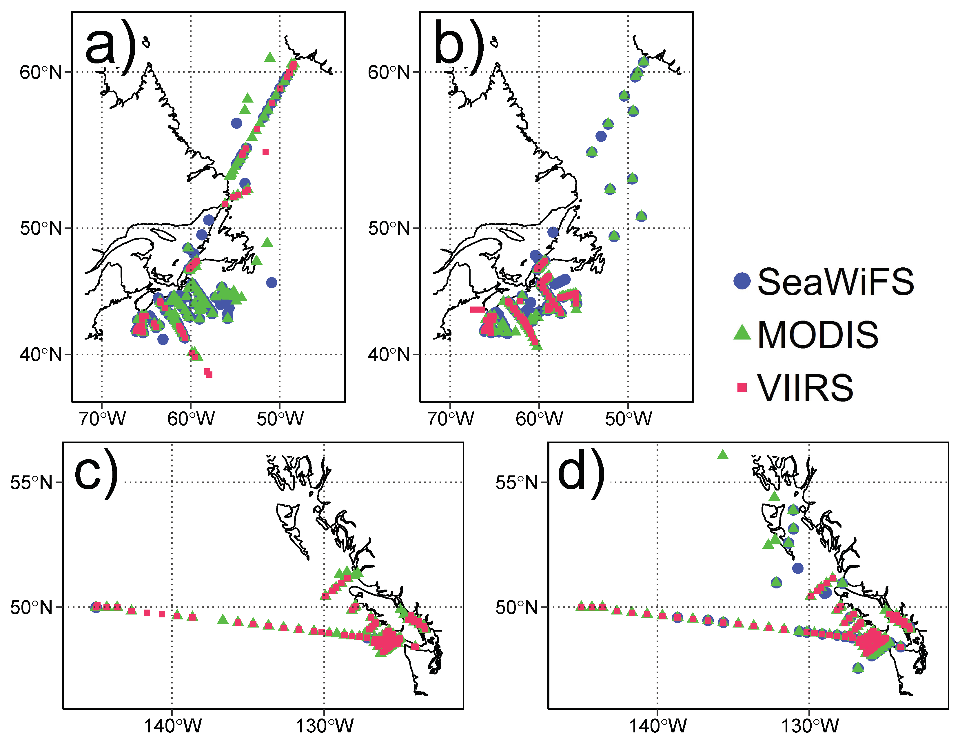
2.1. Regions of Interest
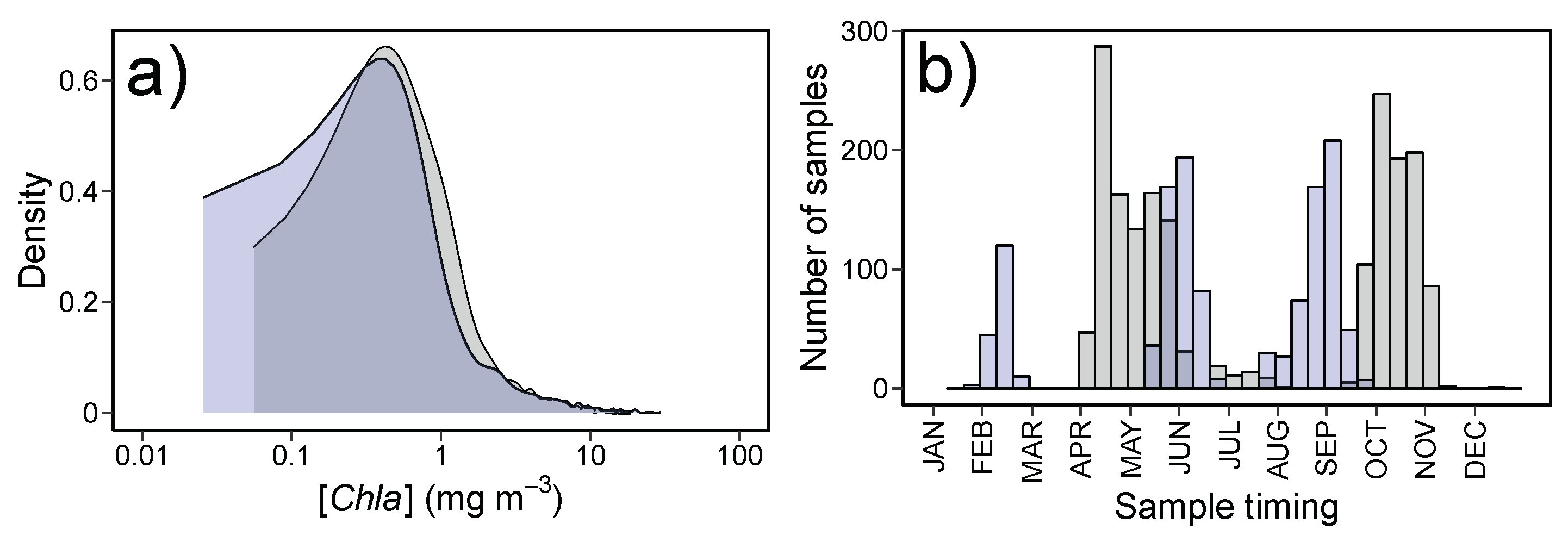
2.2. In Situ Samples
2.3. Satellite Matchups
- The pixel was marked by any of the following level 2 flags: atmospheric correction failure (ATMFAIL), deleted overlapping pixels (BOWTIEDEL), pixel overland (LAND), high sun glint (HIGLINT), pixel contains cloud or ice (CLDICE), radiance too high (HILT), high solar zenith (HISOLZEN), or high sensor zenith angle (HISATZEN).
- The pixel contained a no-data (NA) value.
- The pixel had more than one negative remote sensing reflectance () value, implying the data might be flawed by the atmospheric correction procedure.
2.4. Chlorophyll-a Algorithms
2.4.1. OCx-Type Algorithms
2.4.2. Regional Tuning of the OCx Algorithm
2.4.3. Original GSM
2.4.4. Regional Tuning of GSM
2.5. Performance Metrics
2.5.1. Statistical Models
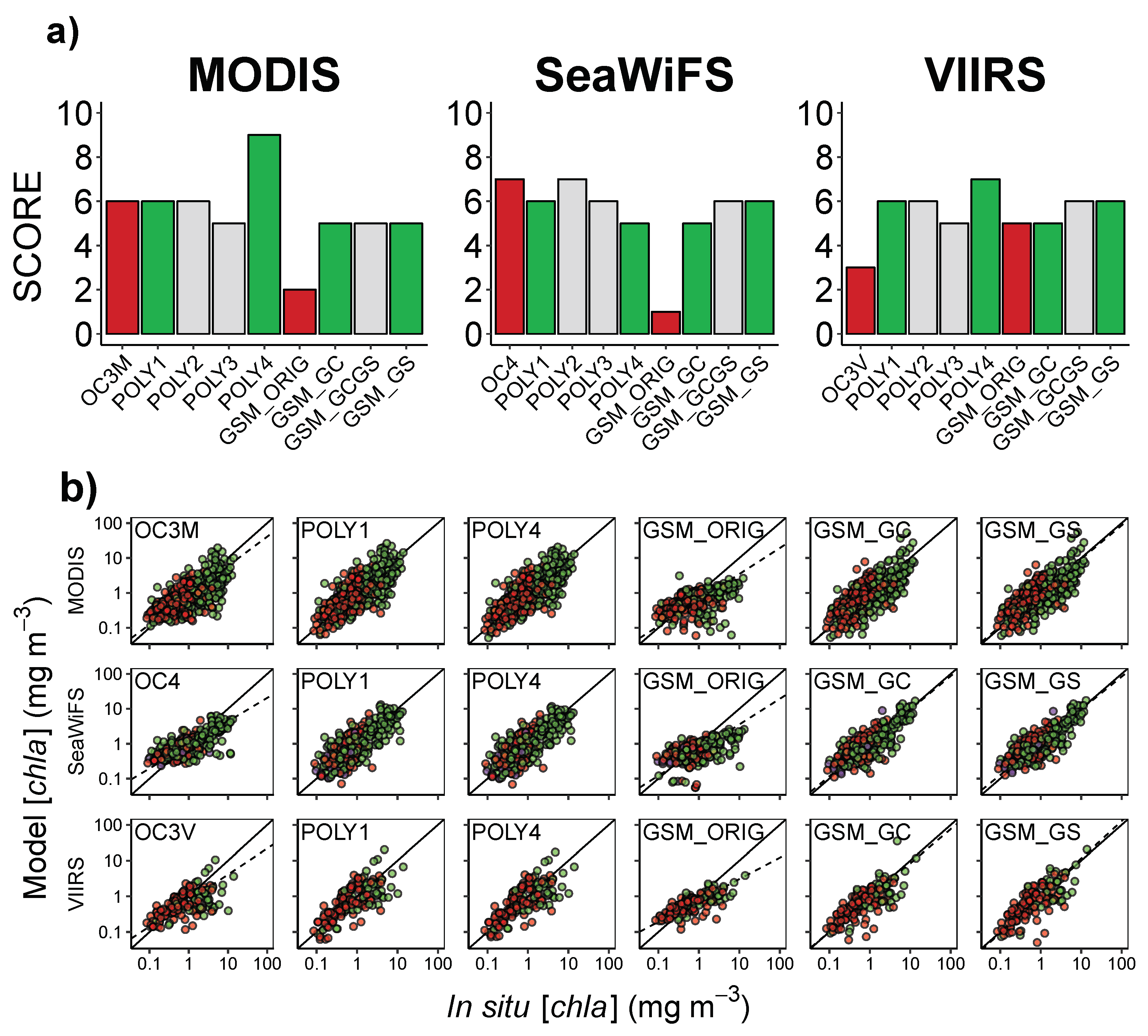
2.5.2. Scoring Method
- , to account for the possible bias in the algorithm,
- , to determine the accuracy of the algorithm,
- of the linear regression, to test the precision or “goodness of fit” of the model,
- percentage of valid retrievals, to ensure that a high score and low error are not reported as a result of a small number of retrievals, and
- win ratio, to judge algorithm performance based on individual matches rather than a summary statistic.
- two points if the algorithm’s transformed statistic was in the lowest 20% of the statistic’s values across all algorithms (i.e., closer to the ideal value of zero) and below the mean,
- zero points if the algorithm’s statistic was in the highest 20% of the statistic’s values across all algorithms (i.e., further from the ideal) and above the mean, and
- one point otherwise
2.6. Temporal, Geographic and Phytoplankton Composition Influences on Algorithm Performance
- time, as defined above (units in decimal year),
- day of year (units in days),
- chlorophyll-a concentration (mg m−3),
- fucoxanthin to chlorophyll-a ratio (unitless),
- latitude (decimal degrees),
- bathymetry in coastal ocean (≤200 m depth, units in metres),
- bathymetry in open ocean (>200 m depth, units in metres), and
- distance (in metres) from central pixel to in situ samples, as we relax the constraint to 10 km.
3. Results
3.1. Parameters of the Optimized Band Ratio Algorithms
3.2. Algorithms performance in the NWA
3.3. Algorithm Performance in the NEP
3.4. Variation of Satellite-Derived with Environmental Factors
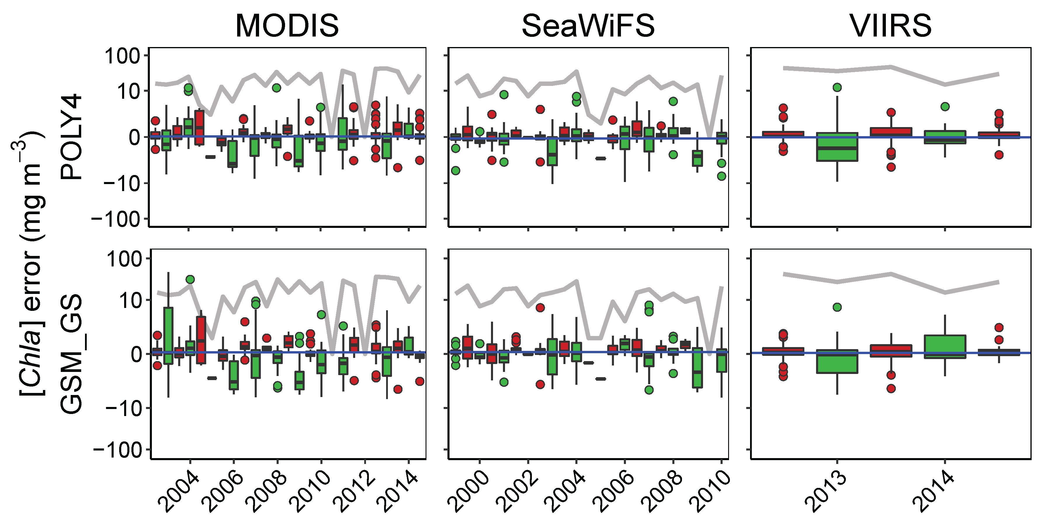
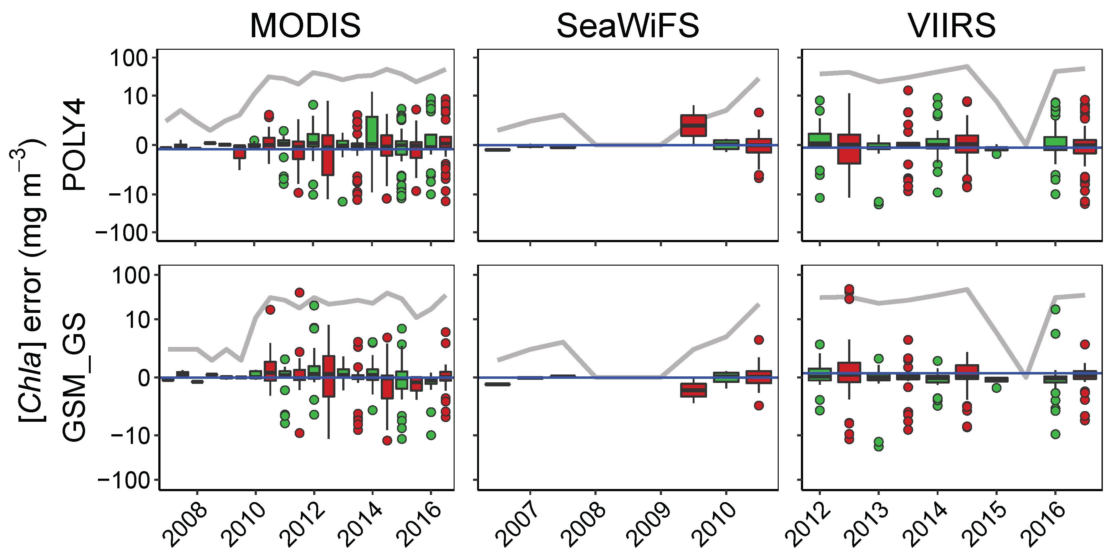
3.4.1. Patterns in Uncertainties with Phytoplankton Composition, Time, and Number of Retrievals
3.4.2. Uncertainties Related to Geographic Considerations
4. Discussion
5. Conclusions
Author Contributions
Funding
Acknowledgments
Conflicts of Interest
Abbreviations
| NWA | Northwest Atlantic |
| NEP | Northeast Pacific |
| SeaWiFS | Sea-viewing Wide Field-of-view Sensor |
| MODIS | Moderate Resolution Imaging Spectrometer |
| VIIRS | Visible Infrared Imaging Radiometer Suite |
| Root mean squared logarithmic error | |
| Mean log-transformed error | |
| Mean magnitude of log-transformed error | |
| OCx | Ocean Colour X |
| GSM | Garver–Siegel Maritorena |
| N | total number of matchups |
| n | number of valid retrievals |
| mean error | |
| coefficient of determination | |
| error in chlorophyll-a concentration retrieval | |
| magnitude of the error in chlorophyll-a concentration retrieval |
Appendix A. Results Omitted from the Main Text

| Algorithm | N | n | Intercept | Slope | RMSLE | MLE | MMLE | Win Ratio | Score | ||
|---|---|---|---|---|---|---|---|---|---|---|---|
| NWA—MODIS | |||||||||||
| POLY2 | 530 | 508 | −1.2 × 10⁻⁵ | 1.00 | 0.57 | 1.3 × 10⁻³ | 0.33 | 1.00 | 1.85 | 0.10 | 6 |
| POLY3 | 530 | 508 | 1.4 × 10⁻⁵ | 1.00 | 0.57 | 0.036 | 0.33 | 1.00 | 1.85 | 0.011 | 5 |
| GSM_GCGS | 530 | 439 | 0.037 | 0.959 | 0.57 | 0.23 | 0.33 | 1.09 | 1.86 | 0.17 | 5 |
| NWA—SeaWiFS | |||||||||||
| POLY2 | 416 | 336 | −5.5 × 10⁻⁷ | 1.00 | 0.62 | −0.10 | 0.31 | 1.00 | 1.74 | 0.068 | 7 |
| POLY3 | 416 | 336 | 1.9 × 10⁻⁵ | 1.00 | 0.62 | −0.077 | 0.31 | 1.00 | 1.73 | 0.076 | 6 |
| GSM_GCGS | 416 | 283 | 0.065 | 0.931 | 0.66 | 0.19 | 0.29 | 1.17 | 1.69 | 0.14 | 6 |
| NWA—VIIRS | |||||||||||
| POLY2 | 176 | 172 | 5.8 × 10⁻⁵ | 1.00 | 0.55 | −0.11 | 0.33 | 1.00 | 1.83 | 0.090 | 6 |
| POLY3 | 176 | 172 | 3.9 × 10⁻⁵ | 1.00 | 0.55 | −0.029 | 0.33 | 1.00 | 1.81 | 6.9 × 10⁻³ | 5 |
| GSM_GCGS | 176 | 154 | 3.7 × 10⁻³ | 0.919 | 0.57 | 0.15 | 0.30 | 1.04 | 1.72 | 0.069 | 6 |
| NEP—MODIS | |||||||||||
| POLY2 | 487 | 461 | −1.9 × 10⁻⁵ | 1.00 | 0.67 | −0.36 | 0.33 | 1.00 | 1.80 | 0.098 | 6 |
| POLY3 | 487 | 461 | 1.4 × 10⁻⁵ | 1.00 | 0.67 | −0.33 | 0.33 | 1.00 | 1.79 | 0.040 | 5 |
| GSM_GCGS | 487 | 355 | 0.039 | 0.975 | 0.69 | 0.16 | 0.29 | 1.10 | 1.66 | 0.16 | 6 |
| NEP—SeaWiFS | |||||||||||
| POLY2 | 45 | 40 | 2.9 × 10⁻⁵ | 1.00 | 0.75 | −0.036 | 0.25 | 1.00 | 1.55 | 0 | 5 |
| POLY3 | 45 | 40 | 2.2 × 10⁻⁷ | 1.00 | 0.75 | −0.071 | 0.25 | 1.00 | 1.55 | 0.21 | 8 |
| GSM_GCGS | 45 | 34 | 0.038 | 0.941 | 0.88 | 0.083 | 0.16 | 1.09 | 1.32 | 0.15 | 5 |
| NEP—VIIRS | |||||||||||
| POLY2 | 342 | 332 | −4.9 × 10⁻⁵ | 1.00 | 0.69 | −0.23 | 0.31 | 1.00 | 1.74 | 0.080 | 7 |
| POLY3 | 342 | 332 | 1.7 × 10⁻⁵ | 1.00 | 0.69 | −0.18 | 0.31 | 1.00 | 1.73 | 0.022 | 5 |
| GSM_GCGS | 342 | 270 | 0.026 | 0.997 | 0.56 | 0.028 | 0.35 | 1.06 | 1.69 | 0.17 | 5 |
| MODIS | SeaWiFS | VIIRS | MODIS | SeaWiFS | VIIRS | |||||||
|---|---|---|---|---|---|---|---|---|---|---|---|---|
| NWA | NEP | |||||||||||
| Algorithm | N | r | N | r | N | r | N | r | N | r | N | r |
| Latitude | ||||||||||||
| POLY2 | 508 | 0.081 | 336 | −0.035 | 172 | 0.38 * | 461 | −0.014 | 40 | 0.21 | 332 | 0.010 |
| POLY3 | 508 | 0.079 | 336 | −0.028 | 172 | 0.34 * | 461 | −0.011 | 40 | 0.22 | 332 | 0.016 |
| GSM_GCGS | 439 | −0.018 | 283 | −0.020 | 155 | 0.19 * | 355 | 2.9 × 10⁻³ | 34 | 0.40 * | 270 | −0.092 |
| Open ocean | ||||||||||||
| POLY2 | 276 | −0.18 * | 171 | −0.13 | 98 | −0.068 | 278 | −0.44 * | 30 | −0.41 * | 197 | −0.46 * |
| POLY3 | 276 | −0.18 * | 171 | −0.13 | 98 | −0.059 | 278 | −0.44 * | 30 | −0.44 * | 197 | −0.46 * |
| GSM_GCGS | 244 | −0.14 * | 149 | −0.13 | 89 | −0.016 | 237 | −0.36 * | 26 | −0.45 * | 179 | −0.35 * |
| Coastal ocean | ||||||||||||
| POLY2 | 232 | −0.024 | 165 | −0.097 | 74 | 0.067 | 186 | −0.090 | 10 | −0.39 | 137 | −0.076 |
| POLY3 | 232 | −0.022 | 165 | −0.10 | 74 | 0.11 | 186 | −0.091 | 10 | −0.41 | 137 | −0.078 |
| GSM_GCGS | 195 | −0.025 | 134 | 0.055 | 66 | 0.20 | 119 | 8.3 × 10⁻³ | 8 | −0.48 | 91 | 0.013 |
| Distance to in situ measurement | ||||||||||||
| POLY2 | 508 | −0.047 | 336 | 0.027 | 172 | −0.080 | 461 | 0.048 | 40 | −0.14 | 332 | 0.053 |
| POLY3 | 508 | −0.049 | 336 | 0.024 | 172 | −0.085 | 461 | 0.049 | 40 | −0.13 | 332 | 0.053 |
| GSM_GCGS | 439 | −0.060 | 283 | −0.077 | 155 | −0.050 | 355 | 0.056 | 34 | −0.35 * | 270 | 0.057 |
| Time | ||||||||||||
| POLY2 | 508 | 1.9 × 10⁻³ | 336 | 0.11 * | 172 | −0.094 | 461 | 0.17 * | 40 | 0.17 | 332 | 0.015 |
| POLY3 | 508 | 2.8 × 10⁻³ | 336 | 0.11 | 172 | −0.089 | 461 | 0.17 * | 40 | 0.21 | 332 | 0.020 |
| GSM_GCGS | 439 | −0.14 * | 283 | 0.14 * | 155 | −0.040 | 355 | −0.020 | 34 | 0.22 | 270 | −0.031 |
| Day of year | ||||||||||||
| POLY2 | 508 | −0.35 * | 336 | −0.26 * | 172 | −0.42 * | 461 | 0.15 * | 40 | 0.12 | 332 | 0.16 * |
| POLY3 | 508 | −0.35 * | 336 | −0.25 * | 172 | −0.41 * | 461 | 0.15 * | 40 | 0.12 | 332 | 0.16 * |
| GSM_GCGS | 439 | −0.20 * | 283 | −0.21 * | 155 | −0.20 * | 355 | 0.11 * | 34 | 0.088 | 270 | 0.094 |
| [Chla] | ||||||||||||
| POLY2 | 508 | 0.64 * | 336 | 0.74 * | 172 | 0.87 * | 461 | 0.84 * | 40 | 0.49 * | 332 | 0.84 * |
| POLY3 | 508 | 0.61 * | 336 | 0.72 * | 172 | 0.75 * | 461 | 0.83 * | 40 | 0.54 * | 332 | 0.82 * |
| GSM_GCGS | 439 | 0.49 * | 283 | 0.65 * | 155 | 0.33 * | 355 | 0.58 * | 34 | 0.39 * | 270 | 0.59 * |
| [Fucox]/[chla] | ||||||||||||
| POLY2 | 508 | 0.30 * | 336 | 0.34 * | 172 | 0.47 * | ||||||
| POLY3 | 508 | 0.29 * | 336 | 0.34 * | 172 | 0.45 * | ||||||
| GSM_GCGS | 439 | 0.25 * | 283 | 0.34 * | 155 | 0.22 * | ||||||
| Algorithm | p-Value | ||||
|---|---|---|---|---|---|
| MODIS | |||||
| OCx | 254 | 239 | −0.86 | 0.074 | 3.3 × 10⁻⁷ * |
| POLY1 | 254 | 239 | −0.077 | 0.26 | 0.14 |
| POLY4 | 254 | 239 | −0.18 | 0.27 | 0.024 * |
| GSM_ORIG | 161 | 179 | −1.7 | −0.11 | 5.5 × 10⁻²⁰ * |
| GSM_GC | 220 | 204 | −0.10 | 0.38 | 0.13 |
| GSM_GS | 221 | 203 | −0.13 | 0.35 | 0.14 |
| SeaWiFS | |||||
| OCx | 183 | 124 | −1.1 | 0.040 | 2.1 × 10⁻⁸ * |
| POLY1 | 183 | 124 | −0.32 | 0.29 | 2.7 × 10⁻³ * |
| POLY4 | 183 | 124 | −0.37 | 0.30 | 5.8 × 10⁻⁴ * |
| GSM_ORIG | 112 | 100 | −1.7 | −0.14 | 3.8 × 10⁻⁹ * |
| GSM_GC | 144 | 109 | −0.17 | 0.32 | 3.7 × 10⁻³ * |
| GSM_GS | 144 | 109 | −0.082 | 0.35 | 0.011 * |
| VIIRS | |||||
| OCx | 51 | 121 | −1.4 | −0.061 | 9.0 × 10⁻⁷ * |
| POLY1 | 51 | 121 | −0.42 | 0.16 | 0.083 |
| POLY4 | 51 | 121 | −0.48 | 0.17 | 0.038 * |
| GSM_ORIG | 39 | 105 | −1.2 | −0.16 | 1.0 × 10⁻⁵ * |
| GSM_GC | 42 | 111 | 0.047 | −0.036 | 0.87 |
| GSM_GS | 42 | 111 | −0.098 | 0.11 | 0.33 |
| Algorithm | p-Value | |||||||||
|---|---|---|---|---|---|---|---|---|---|---|
| MODIS | ||||||||||
| OCx | 87 | 194 | 135 | −0.28 | 0.23 | −0.20 | 0.47 | 0.56 | 0.99 | 0.58 |
| POLY1 | 87 | 194 | 135 | −0.37 | −0.054 | −0.38 | 0.63 | 0.75 | 1.0 | 0.67 |
| POLY4 | 87 | 194 | 135 | −0.40 | −0.14 | −0.44 | 0.69 | 0.82 | 1.00 | 0.71 |
| GSM_ORIG | 47 | 139 | 58 | −1.5 | −0.89 | −1.3 | 0.39 | 0.41 | 0.91 | 0.66 |
| GSM_GC | 65 | 155 | 97 | 0.35 | 0.13 | 0.065 | 0.89 | 0.92 | 0.89 | 0.99 |
| GSM_GS | 64 | 154 | 97 | 0.24 | −0.020 | −0.20 | 0.75 | 0.87 | 0.73 | 0.92 |
| VIIRS | ||||||||||
| OCx | 67 | 115 | 116 | −0.89 | 0.014 | −0.51 | 0.34 | 0.34 | 0.83 | 0.60 |
| POLY1 | 67 | 115 | 116 | −0.70 | 0.17 | −0.093 | 0.32 | 0.29 | 0.55 | 0.85 |
| POLY4 | 67 | 115 | 116 | −0.80 | 0.12 | −0.11 | 0.23 | 0.21 | 0.41 | 0.87 |
| GSM_ORIG | 36 | 93 | 74 | −1.5 | −0.48 | −1.4 | 0.085 | 0.19 | 0.98 | 0.14 |
| GSM_GC | 52 | 99 | 83 | −0.52 | 0.30 | 0.29 | 0.42 | 0.44 | 0.47 | 1.0 |
| GSM_GS | 52 | 101 | 83 | −0.68 | 0.97 | −0.042 | 0.16 | 0.17 | 0.78 | 0.41 |
| Algorithm | N | p-Value | N | p-Value | ||||||
|---|---|---|---|---|---|---|---|---|---|---|
| Coastal | Open | Coastal | Open | Coastal | Open | Coastal | Open | |||
| NWA | NEP | |||||||||
| MODIS | ||||||||||
| OCx | 232 | 276 | −0.27 | −0.51 | 0.20 | 183 | 275 | −0.46 | 0.18 | 0.064 |
| POLY1 | 232 | 276 | 0.42 | −0.20 | 4.9 × 10⁻³ * | 183 | 275 | −0.78 | 0.083 | 4.6 × 10⁻³ * |
| POLY4 | 232 | 276 | 0.32 | −0.20 | 6.7 × 10⁻³ * | 183 | 275 | −0.90 | 0.076 | 8.4 × 10⁻⁴ * |
| GSM_ORIG | 142 | 212 | −1.0 | −0.71 | 0.077 | 77 | 201 | −2.4 | −0.41 | 7.3 × 10⁻⁹ * |
| GSM_GC | 195 | 244 | 0.36 | −0.066 | 0.17 | 118 | 237 | 0.17 | 0.12 | 0.91 |
| GSM_GS | 195 | 244 | 0.33 | −0.090 | 0.19 | 118 | 236 | −0.093 | 0.016 | 0.77 |
| SeaWiFS | ||||||||||
| OCx | 165 | 171 | −0.53 | −0.64 | 0.55 | 10 | 30 | −0.17 | −0.40 | 0.69 |
| POLY1 | 165 | 171 | 0.19 | −0.30 | 6.9 × 10⁻³ * | 10 | 30 | 0.36 | −0.12 | 0.39 |
| POLY4 | 165 | 171 | 0.14 | −0.31 | 0.011 * | 10 | 30 | 0.37 | −0.13 | 0.35 |
| GSM_ORIG | 107 | 132 | −1.1 | −0.72 | 0.17 | 8 | 25 | −1.1 | −0.20 | 0.032 * |
| GSM_GC | 134 | 148 | 0.24 | −0.11 | 0.029 * | 8 | 26 | 0.19 | −0.047 | 0.44 |
| GSM_GS | 134 | 148 | 0.34 | −0.091 | 7.1 × 10⁻³ * | 8 | 26 | 0.36 | −0.12 | 0.17 |
| VIIRS | ||||||||||
| OCx | 74 | 98 | −0.23 | −0.61 | 0.13 | 135 | 195 | −1.1 | 0.12 | 4.5 × 10⁻³ * |
| POLY1 | 74 | 98 | 0.40 | −0.32 | 0.021 | 135 | 195 | −0.77 | 0.27 | 9.0 × 10⁻³ * |
| POLY4 | 74 | 98 | 0.36 | −0.31 | 0.020 | 135 | 195 | −0.87 | 0.26 | 2.4 × 10⁻³ * |
| GSM_ORIG | 57 | 87 | −0.47 | −0.43 | 0.87 | 69 | 161 | −2.3 | −0.28 | 5.5 × 10⁻⁷ * |
| GSM_GC | 64 | 89 | 0.26 | −0.21 | 0.29 | 88 | 177 | 0.29 | 3.7 × 10⁻⁴ | 0.56 |
| GSM_GS | 64 | 89 | 0.010 | 0.085 | 0.70 | 89 | 177 | 0.77 | −0.069 | 0.20 |
| POLY4 | GSM_GS | POLY4 | GSM_GS | POLY4 | GSM_GS | |
|---|---|---|---|---|---|---|
| MODIS | SeaWiFS | VIIRS | ||||
| NWA | ||||||
| January–June | 1.7 | 2.0 | 1.1 | 0.94 | 1.7 | 1.5 |
| July–December | 0.74 | 0.84 | 0.57 | 0.60 | 0.46 | 0.44 |
| NEP | ||||||
| January–June | 0.65 | 0.37 | 0.33 | 0.27 | 0.54 | 0.37 |
| July–December | 1.0 | 0.72 | 0.94 | 0.38 | 1.1 | 0.62 |
| Coefficients | MODIS | SeaWiFS | VIIRS | |||
|---|---|---|---|---|---|---|
| POLY2 | POLY3 | POLY2 | POLY3 | POLY2 | POLY3 | |
| NWA | ||||||
| a | 0.37539 | 0.37657 | 0.51424 | 0.52039 | 0.41461 | 0.44156 |
| b | −3.12409 | −3.26173 | −3.59265 | −3.75269 | −2.54637 | −3.05795 |
| c | −0.75408 | −0.60435 | −0.95058 | −0.92392 | −1.47087 | −0.65894 |
| d | - | 1.1404 | - | 1.71524 | - | 1.21248 |
| e | - | - | - | - | - | - |
| NEP | ||||||
| a | 0.28424 | 0.2805 | 0.42171 | 0.42506 | 0.33771 | 0.3303 |
| b | −2.66996 | −2.77728 | −2.95509 | −2.74285 | −2.56462 | −2.74252 |
| c | −1.09915 | −1.01747 | −0.68104 | −1.48743 | −0.5314 | −0.34545 |
| d | - | 0.92282 | - | 0.17624 | - | 1.35569 |
| e | - | - | - | - | - | - |
| 400 | 0.0742 | 0.0805 | 1.4839 |
| 410 | 0.0716 | 0.0820 | 1.4520 |
| 420 | 0.0697 | 0.0841 | 1.4353 |
| 430 | 0.0685 | 0.0862 | 1.4300 |
| 440 | 0.0697 | 0.0890 | 1.4595 |
| 450 | 0.0773 | 0.1009 | 1.6387 |
| 460 | 0.0801 | 0.1142 | 1.7489 |
| 470 | 0.0832 | 0.1394 | 1.9055 |
| 480 | 0.0869 | 0.2095 | 2.1890 |
| 490 | 0.0878 | 0.2621 | 2.3091 |
| 500 | 0.0875 | 0.2820 | 2.3212 |
| 510 | 0.0861 | 0.2568 | 2.2215 |
| 520 | 0.0844 | 0.2233 | 2.1058 |
| 530 | 0.0821 | 0.1967 | 1.9920 |
| 540 | 0.0800 | 0.1811 | 1.9097 |
| 550 | 0.0781 | 0.1717 | 1.8464 |
| 560 | 0.0763 | 0.1651 | 1.7968 |
| 570 | 0.0754 | 0.1624 | 1.7722 |
| 580 | 0.0757 | 0.1640 | 1.7816 |
| 590 | 0.0768 | 0.1712 | 1.8211 |
| 600 | 0.0781 | 0.1864 | 1.8879 |
| 610 | 0.0784 | 0.1939 | 1.9143 |
| 620 | 0.0783 | 0.1956 | 1.9172 |
| 630 | 0.0782 | 0.1969 | 1.9186 |
| 640 | 0.0780 | 0.1973 | 1.9160 |
| 650 | 0.0782 | 0.2009 | 1.9283 |
| 660 | 0.0789 | 0.2227 | 1.9923 |
| 670 | 0.0798 | 0.2513 | 2.0663 |
| 680 | 0.0795 | 0.2465 | 2.0510 |
| 690 | 0.0789 | 0.2270 | 2.0000 |
| 700 | 0.0791 | 0.2323 | 2.0137 |
| MODIS | SeaWiFS | VIIRS | MODIS | SeaWiFS | VIIRS | |||||||
|---|---|---|---|---|---|---|---|---|---|---|---|---|
| NWA | NEP | |||||||||||
| median P | 0.500 | 0.500 | 0.500 | 0.500 | 0.600 | 0.500 | 0.600 | 0.600 | 0.700 | 0.650 | 0.600 | 0.600 |
| median S | 0.038 | 0.036 | 0.035 | 0.034 | 0.026 | 0.026 | 0.038 | 0.036 | 0.028 | 0.026 | 0.034 | 0.030 |
| median Y | 0.800 | 0.750 | 0.600 | 0.525 | 1.400 | 1.750 | 0.900 | 0.750 | 0.750 | 0.650 | 0.800 | 0.750 |
| 410 | 0.054343 |
| 412 | 0.055765 |
| 443 | 0.063252 |
| 469 | 0.051276 |
| 486 | 0.04165 |
| 488 | 0.040648 |
| 490 | 0.039546 |
| 510 | 0.025105 |
| 531 | 0.015745 |
| 547 | 0.011477 |
| 551 | 0.010425 |
| 555 | 0.009382 |
| 645 | 0.008967 |
| 667 | 0.019878 |
| 670 | 0.022861 |
| 671 | 0.023646 |
| 678 | 0.024389 |
References
- Vargas, M.; Brown, C.W.; Sapiano, M.R.P. Phenology of marine phytoplankton from satellite ocean color measurements. Geophys. Res. Lett. 2009, 36. [Google Scholar] [CrossRef]
- Racault, M.F.; Quéré, C.L.; Buitenhuis, E.; Sathyendranath, S.; Platt, T. Phytoplankton phenology in the global ocean. Ecol. Indic. 2012, 14, 152–163. [Google Scholar] [CrossRef]
- Siegel, D.A.; Buesseler, K.O.; Doney, S.C.; Sailley, S.F.; Behrenfeld, M.J.; Boyd, P.W. Global assessment of ocean carbon export by combining satellite observations and food-web models. Glob. Biogeochem. Cycles 2014, 28, 181–196. [Google Scholar] [CrossRef]
- Toming, K.; Kutser, T.; Uiboupin, R.; Arikas, A.; Vahter, K.; Paavel, B. Mapping Water Quality Parameters with Sentinel-3 Ocean and Land Colour Instrument imagery in the Baltic Sea. Remote Sens. 2017, 9, 1070. [Google Scholar] [CrossRef]
- Natvik, L.J.; Evensen, G. Assimilation of ocean colour data into a biochemical model of the North Atlantic: Part 1. Data assimilation experiments. J. Mar. Syst. 2003, 40–41, 127–153. [Google Scholar] [CrossRef]
- IOCCG. Remote Sensing in Fisheries and Aquaculture; Reports of the International Ocean Colour Coordinating Group; IOCCG: Dartmouth, NS, Canada, 2009; Volume 8. [Google Scholar] [CrossRef]
- McIver, R.; Breeze, H.; Devred, E. Satellite remote-sensing observations for definitions of areas for marine conservation: Case study of the Scotian Slope, Eastern Canada. Remote Sens. Environ. 2018, 214. [Google Scholar] [CrossRef]
- Johnson, C.; Devred, E.; Casault, B.; Head, E.; Cogswell, A.; Spry, J. Optical, Chemical, and Biological Oceanographic Conditions on the Scotian Shelf and in the Eastern Gulf of Maine during 2015. Available online: http://publications.gc.ca/site/eng/9.833512/publication.html (accessed on 5 November 2019).
- Hannah, C.G.; McKinnell, S. (Eds.) Applying Remote Sensing Data to Fisheries Management in BC; Technical Report; Department of Fisheries and Oceans Canada: Ottawa, ON, Canada, 2016.
- O’Reilly, J.E.; Maritorena, S.; Mitchell, B.G.; Siegel, D.A.; Carder, K.L.; Garver, S.A.; Kahru, M.; McClain, C. Ocean color chlorophyll algorithm for SeaWiFS. J. Geophys. Res. 1998, 103, 24937–24953. [Google Scholar] [CrossRef]
- Werdell, J.; Franz, B.; Bailey, S.; Feldman, G.; Boss, E.; Brando, V.; Dowell, M.; Hirata, T.; Lavender, S.; Lee, Z.; et al. Generalized ocean color inversion model for retrieving marine inherent optical properties. Appl. Opt. 2013, 52, 2019–2037. [Google Scholar] [CrossRef]
- Werdell, P.J.; Bailey, S.W. An improved in situ bio-optical dataset for ocean colour algorithm development and satellite data production validation. Remote Sens. Environ. 2005, 98, 122–140. [Google Scholar] [CrossRef]
- Gower, J. On the use of satellite-measured chlorophyll fluorescence for monitoring coastal waters. Int. J. Remote Sens. 2015. [Google Scholar] [CrossRef]
- Doerffer, R.; Schiller, H. The MERIS case 2 water algorithm. Int. J. Remote Sens. 2007, 28, 517–535. [Google Scholar] [CrossRef]
- Laliberté, J.; Larouche, P.; Devred, E.; Craig, S. Chlorophyll-a Concentration Retrieval in the Optically Complex Waters of the St. Lawrence Estuary and Gulf Using Principal Component Analysis. Remote Sens. 2018, 10, 265. [Google Scholar] [CrossRef]
- Hamed, G.; Scott, R. Revisiting empirical ocean-colour algorithms for remote estimation of chlorophyll-a content on a global scale. Int. J. Remote Sens. 2016, 37, 2682–2705. [Google Scholar] [CrossRef]
- Ben Mustapha, S.; Bélanger, S.; Larouche, P. Evaluation of ocean color algorithms in the southeastern Beaufort Sea, Canadian Arctic: New parameterization using SeaWiFS, MODIS, and MERIS spectral bands. Can. J. Remote Sens. 2012, 38, 535–556. [Google Scholar] [CrossRef]
- Peña, A.; Nemcek, N. Phytoplankton in Surface Waters along Line P and off the West Coast of Vancouver Island. In State of the Physical, Biological and Selected Fishery Resources of Pacific Canadian Marine Ecosystems in 2017; Chandler, P.C., King, S.A., Boldt, J., Eds.; Can. Tech. Rep. Fish. Aquat. Sci.; 2018; Volume 3266, pp. 55–59. Available online: http://waves-vagues.dfo-mpo.gc.ca/Library/40717914.pdf (accessed on 5 November 2019).
- Head, E.J.H.; Horne, E.P.W. Pigment transformation and vertical flux in an area of convergence in the North Atlantic. Deep-Sea Res. II 1993, 40, 329–346. [Google Scholar] [CrossRef]
- Stuart, V.; Head, E.J.H. The BIO method. In The Second SeaWiFS HPLC Analysis Round-Robin Experiment (SeaHARRE-2); NASA/TM 2005-212785; Hooker, S.B., Ed.; NASA, Goddard Space Flight Center: Greenbelt, MD, USA, 2005; p. 112. [Google Scholar]
- Zapata, M.; Rodríguez, F.; Garrido, J. Separation of chlorophylls and carotenoids from marine phytoplankton: A new HPLC method using a reversed phase C8 column and pyridine-containing mobile phases. Mar. Ecol. Prog. Ser. 2000, 195, 29–45. [Google Scholar] [CrossRef]
- Hijmans, R.J. Geosphere: Spherical Trigonometry (R Package Version 1.5-7). 2017. Available online: http://cran.nexr.com/web/packages/geosphere/index.html (accessed on 5 November 2019).
- Maritorena, S.; Siegel, D.A.; Peterson, A.R. Optimization of a semi-analytical ocean color model for global-scale applications. Appl. Opt. 2002, 41, 2705–2713. [Google Scholar] [CrossRef]
- R Core Team. R: A Language and Environment for Statistical Computing; R Foundation for Statistical Computing: Vienna, Austria, 2016. [Google Scholar]
- Davison, A.C.; Hinkley, D.V. Bootstrap Methods and Their Applications; Cambridge University Press: Cambridge, UK, 1997; ISBN 0-521-57391-2. [Google Scholar]
- Canty, A.; Ripley, B.D. Boot: Bootstrap R (S-Plus) Functions (R Package Version 1.3-22). 2019. Available online: https://cran.rapporter.net/bin/linux/ubuntu/disco-cran35/Packages (accessed on 5 November 2019).
- Garver, S.A.; Siegel, D.A. Inherent optical property inversion of ocean color spectra and its biogeochemical interpretation: 1. Time series from the Sargasso Sea. J. Geophys. Res. Oceans 1997, 102, 18607–18625. [Google Scholar] [CrossRef]
- Gordon, H.R.; Brown, J.W.; Evans, R.H.; Brown, J.W.; Smith, R.C.; Baker, K.S.; Clark, D.K. A semianalytic radiance model of ocean color. J. Geophys. Res. 1988, 93, 10909–10924. [Google Scholar] [CrossRef]
- Pope, R.M.; Fry, E.S. Absorption spectrum (380–700 nm) of pure water. II. Integrating measurements. Appl. Opt. 1997, 36, 8710–8723. [Google Scholar] [CrossRef]
- Smith, R.; Baker, K. Optical properties of the clearest natural waters (200–800 nm). Appl. Opt. 1981, 20, 177–184. [Google Scholar] [CrossRef] [PubMed]
- IOCCG. Remote Sensing of Inherent Optical Properties: Fundamentals, Tests of Algorithms, and Applications; Reports of the International Oean-Colour Coordinating Group, No. 5; Lee, Z.P., Ed.; IOCCG: Dartmouth, NS, Canada, 2006. [Google Scholar]
- Lee, Z.P.; Carder, K.L.; Arnone, R. Deriving inherent optical properties from water color: A multi-band quasi-analytical algorithm for optically deep waters. Appl. Opt. 2002, 41, 5755–5772. [Google Scholar] [CrossRef] [PubMed]
- Bricaud, A.; Claustre, H.; Oubelkheir, K. Natural variability of phytoplankton absorption in oceanic waters: influence of the size structure of algal populations. J. Geophys. Res. 2004, 110. [Google Scholar] [CrossRef]
- Legendre, P. Lmodel2: Model II Regression (R Package Version 1.7-3). 2018. Available online: https://cran.r-project.org/web/packages/lmodel2/index.html (accessed on 5 November 2019).
- Seegers, B.; Stumpf, R.; Schaeffer, B.; Loftin, K.; Werdell, J. Performance metrics for the assessment of satellite data products: An ocean color case study. Opt. Express 2018, 26, 7404. [Google Scholar] [CrossRef] [PubMed]
- Brewin, B.; Sathyendranath, S.; Müller, D.; Brockmann, C.; Deschamps, P.Y.; Devred, E.; Doerffer, R.; Fomferra, N.; Franz, B.; Grant, M.; et al. The Ocean Colour Climate Change Initiative: III. A round-robin comparison on in-water bio-optical algorithms. Remote Sens. Environ. 2015, 162. [Google Scholar] [CrossRef]
- Wickham, H. ggplot2: Elegant Graphics for Data Analysis; Springer: New York, NY, USA, 2009. [Google Scholar]
- Claustre, H. The trophic status of various oceanic provinces as revealed by phytoplankton pigment signatures. Limnol. Oceanogr. 1994, 39, 1206–1210. [Google Scholar] [CrossRef]
- Jeffrey, S.W.; Vesk, M. Introduction to marine phytoplankton and their pigment signature. In Phytoplankton Pigments in Oceanography: Guidelines to Modern Methods; Jeffrey, S.W., Mantoura, R.F.C., Wright, S.W., Eds.; UNESCO Publishing: Paris, France, 1997; pp. 37–84. [Google Scholar]
- Garcia, V.M.T.; Signorini, S.; Garcia, C.A.E.; McClain, C.R. Empirical and semi-analytical chlorophyll algorithms in the south-western Atlantic coastal region (25–40°S and 60–45°W). Int. J. Remote Sens. 2006, 27, 1539–1562. [Google Scholar] [CrossRef]
- Sun, L.; Guo, M.; Wang, X. Ocean color products retrieval and validation around China coast with MODIS. Acta Oceanol. Sin. 2010, 29, 21–27. [Google Scholar] [CrossRef]
- Jiang, W.; Knight, B.R.; Cornelisen, C.; Barter, P.; Kudela, R. Simplifying Regional Tuning of MODIS Algorithms for Monitoring Chlorophyll-a in Coastal Waters. Front. Mar. Sci. 2017, 4, 151. [Google Scholar] [CrossRef]
- Hooker, S.B.; Esaias, W.E.; Feldman, G.C.; Gregg, W.W.; McClain, C.R. An Overview of SeaWiFS and Ocean Color; Tech. Memo. 104566; Hooker, S., Firestone, E., Eds.; NASA Goddard Space Flight Center: Greenbelt, MD, USA, 1992; Volume 1, 24p.
- Eplee, R.E.; Robinson, W.D.; Bailey, S.W.; Clark, D.K.; Werdell, P.J.; Wang, M.; Barnes, R.A.; McClain, C.R. Calibration of SeaWiFS. II. Vicarious techniques. Appl. Opt. 2001, 40, 6701–6718. [Google Scholar] [CrossRef]
- Stuart, V.; Sathyendranath, S.; Platt, T.; Maass, H.; Irwin, B.D. Pigments and species compositon of natural phytoplankton populations: effect on the absorption spectra. J. Plankton Res. 1998, 20, 187–217. [Google Scholar] [CrossRef]
- Sathyendranath, S.; Cota, G.; Stuart, V.; Maass, H.; Platt, T. Remote sensing of phytoplankton pigments: A comparison of empirical and theoretical approaches. Int. J. Remote Sens. 2001, 22, 249–273. [Google Scholar] [CrossRef]
- Devred, E.; Sathyendranath, S.; Stuart, V.; Maass, H.; Ulloa, O.; Platt, T. A two-component model of phytoplankton absorption in the open ocean: theory and applications. J. Geophys. Res. 2006, 111. [Google Scholar] [CrossRef]
- Sathyendranath, S.; Watts, L.; Devred, E.; Platt, T.; Caverhill, C.; Maass, H. Discrimination of diatoms from other phytoplankton using ocean-colour data. Mar. Ecol. Prog. Ser. 2004, 272, 59–68. [Google Scholar] [CrossRef]
- IOCCG. Atmospheric Correction for Remotely-Sensed Ocean-Colour Products; Reports of the International Ocean Colour Coordinating Group; IOCCG: Dartmouth, NS, Canada, 2010; Volume 10. [Google Scholar] [CrossRef]
- Morel, A.; Prieur, L. Analysis of variation in ocean color. Limnol. Oceanogr. 1977, 22, 709–722. [Google Scholar] [CrossRef]
- Carswell, T.; Costa, M.; Young, E.; Komick, N.; Gower, J.; Sweeting, R. Evaluation of MODIS-Aqua Atmospheric Correction and Chlorophyll Products of Western North American Coastal Waters Based on 13 Years of Data. Remote Sens. 2017, 9, 1063. [Google Scholar] [CrossRef]


| Sensor | Resolution | Wavebands | Period | N | Period | N |
|---|---|---|---|---|---|---|
| (km) | (nm) | (Year) | (Year) | |||
| NWA | NEP | |||||
| MODIS | 1.1 | 412, 443, 469, 488, 531, 547, 555, 645, 667, 678 | 2002–2014 | 530 | 2006–2016 | 487 |
| SeaWiFS | 1.0 | 412, 443, 490, 510, 555, 670 | 1999–2010 | 416 | 2006–2010 | 45 |
| VIIRS | 0.75 | 410, 443, 486, 551, 671 | 2012–2014 | 176 | 2012–2016 | 342 |
| Coefficients | MODIS | SeaWiFS | VIIRS | ||||||
|---|---|---|---|---|---|---|---|---|---|
| OC3M | POLY1 | POLY4 | OC4 | POLY1 | POLY4 | OC3V | POLY1 | POLY4 | |
| NWA | |||||||||
| a | 0.2424 | 0.36695 | 0.37925 | 0.3272 | 0.51664 | 0.51824 | 0.2228 | 0.43399 | 0.44786 |
| b | −2.7423 | −3.27757 | −3.28487 | −2.9940 | −3.84589 | −3.68431 | −2.4683 | −3.09652 | −3.11091 |
| c | 1.8017 | - | −0.75830 | 2.7218 | - | −0.97401 | 1.5867 | - | −0.77987 |
| d | 0.0015 | - | 1.49122 | −1.2259 | - | 0.84875 | −0.4275 | - | 1.42500 |
| e | −1.2280 | - | 0.80020 | −0.5683 | - | 0.77874 | −0.7768 | - | 0.90445 |
| NEP | |||||||||
| a | 0.24947 | 0.26575 | 0.41867 | 0.42516 | 0.31886 | 0.33055 | |||
| b | −2.84152 | −2.84142 | −3.14708 | −3.14271 | −2.65010 | −2.76455 | |||
| c | - | −0.57938 | - | −0.70269 | - | −0.39595 | |||
| d | - | 0.74974 | - | 1.21802 | - | 1.52198 | |||
| e | - | 0.47743 | - | 1.59686 | - | 0.46509 | |||
| Algorithm | N | n | Intercept | Slope | RMSLE | MLE | MMLE | Win Ratio | Score | ||
|---|---|---|---|---|---|---|---|---|---|---|---|
| MODIS | |||||||||||
| OC3M | 530 | 508 | −0.067 | 0.839 | 0.45 | −0.40 | 0.37 | 0.857 | 1.95 | 0.15 | 6 |
| POLY1 | 530 | 508 | −1.0 | 1.00 | 0.57 | 0.081 | 0.34 | 1.00 | 1.85 | 0.037 | 6 |
| POLY4 | 530 | 508 | −4.2 | 1.00 | 0.57 | 0.037 | 0.33 | 1.00 | 1.85 | 0.083 | 9 |
| GSM_ORIG | 530 | 354 | −0.21 | 0.745 | 0.22 | −0.84 | 0.47 | 0.644 | 2.16 | 0.32 | 2 |
| GSM_GC | 530 | 439 | 5.7 | 0.995 | 0.56 | 0.13 | 0.34 | 1.01 | 1.88 | 0.10 | 5 |
| GSM_GS | 530 | 439 | 7.3 | 0.963 | 0.57 | 0.10 | 0.33 | 1.02 | 1.86 | 0.023 | 5 |
| SeaWiFS | |||||||||||
| OC4 | 416 | 336 | −0.035 | 0.674 | 0.55 | −0.58 | 0.32 | 0.928 | 1.75 | 0.25 | 7 |
| POLY1 | 416 | 336 | 1.1 | 1.00 | 0.62 | −0.062 | 0.31 | 1.00 | 1.72 | 0.093 | 6 |
| POLY4 | 416 | 336 | −1.2 | 1.00 | 0.62 | −0.087 | 0.31 | 1.00 | 1.73 | 4.2 | 5 |
| GSM_ORIG | 416 | 239 | −0.18 | 0.734 | 0.28 | −0.87 | 0.44 | 0.681 | 2.15 | 0.23 | 1 |
| GSM_GC | 416 | 282 | 0.025 | 0.957 | 0.64 | 0.057 | 0.29 | 1.06 | 1.69 | 0.11 | 5 |
| GSM_GS | 416 | 282 | 0.044 | 0.938 | 0.66 | 0.11 | 0.29 | 1.11 | 1.68 | 0.034 | 6 |
| VIIRS | |||||||||||
| OC3V | 176 | 172 | −0.12 | 0.728 | 0.38 | −0.45 | 0.37 | 0.831 | 1.90 | 0.13 | 3 |
| POLY1 | 176 | 172 | 3.1 | 1.00 | 0.55 | −8.7 | 0.33 | 1.00 | 1.82 | 0.035 | 6 |
| POLY4 | 176 | 172 | 1.1 | 1.00 | 0.55 | −0.018 | 0.33 | 1.00 | 1.81 | 0.15 | 7 |
| GSM_ORIG | 176 | 144 | −0.12 | 0.600 | 0.55 | −0.45 | 0.31 | 0.906 | 1.78 | 0.24 | 5 |
| GSM_GC | 176 | 153 | −0.036 | 0.959 | 0.56 | −0.013 | 0.32 | 0.934 | 1.74 | 0.069 | 5 |
| GSM_GS | 176 | 153 | 0.018 | 1.04 | 0.58 | 0.054 | 0.32 | 1.02 | 1.75 | 0.21 | 6 |
| Algorithm | N | n | Intercept | Slope | RMSLE | MLE | MMLE | Win Ratio | Score | ||
|---|---|---|---|---|---|---|---|---|---|---|---|
| MODIS | |||||||||||
| OC3M | 487 | 461 | 0.021 | 0.966 | 0.59 | −0.016 | 0.37 | 1.05 | 1.87 | 0.12 | 5 |
| POLY1 | 487 | 461 | −5.3 | 1.00 | 0.66 | −0.21 | 0.34 | 1.00 | 1.78 | 0.11 | 7 |
| POLY4 | 487 | 461 | 1.2 | 1.00 | 0.67 | −0.27 | 0.33 | 1.00 | 1.79 | 0.040 | 5 |
| GSM_ORIG | 487 | 279 | −0.18 | 0.729 | 0.55 | −0.96 | 0.37 | 0.708 | 1.81 | 0.28 | 3 |
| GSM_GC | 487 | 356 | 0.011 | 1.02 | 0.69 | 0.14 | 0.30 | 1.02 | 1.67 | 0.11 | 5 |
| GSM_GS | 487 | 355 | 2.1 | 0.968 | 0.69 | −0.013 | 0.29 | 1.01 | 1.65 | 0.040 | 5 |
| SeaWiFS | |||||||||||
| OC4 | 45 | 40 | −0.042 | 0.851 | 0.63 | −0.34 | 0.30 | 0.897 | 1.65 | 0.15 | 3 |
| POLY1 | 45 | 40 | −1.3 | 1.00 | 0.75 | −3.8 | 0.25 | 1.00 | 1.55 | 0.030 | 6 |
| POLY4 | 45 | 40 | 5.3 | 1.00 | 0.75 | −5.5 | 0.25 | 1.00 | 1.54 | 0.091 | 6 |
| GSM_ORIG | 45 | 33 | −0.028 | 0.634 | 0.81 | −0.42 | 0.23 | 0.959 | 1.56 | 0.15 | 4 |
| GSM_GC | 45 | 34 | 0.017 | 0.958 | 0.88 | 9.0 | 0.16 | 1.04 | 1.30 | 0 | 6 |
| GSM_GS | 45 | 34 | 4.4 | 0.972 | 0.87 | −0.010 | 0.17 | 1.01 | 1.32 | 0.21 | 6 |
| VIIRS | |||||||||||
| OC3V | 342 | 332 | −0.042 | 0.930 | 0.63 | −0.36 | 0.34 | 0.902 | 1.78 | 0.17 | 6 |
| POLY1 | 342 | 332 | 7.7 | 1.00 | 0.69 | −0.13 | 0.32 | 1.00 | 1.74 | 0.045 | 7 |
| POLY4 | 342 | 332 | 1.4 | 1.00 | 0.69 | −0.17 | 0.31 | 1.00 | 1.74 | 0.063 | 6 |
| GSM_ORIG | 342 | 230 | −0.10 | 0.725 | 0.48 | −0.88 | 0.38 | 0.831 | 1.80 | 0.25 | 2 |
| GSM_GC | 342 | 265 | 0.021 | 1.01 | 0.68 | 0.095 | 0.29 | 1.05 | 1.60 | 0.13 | 6 |
| GSM_GS | 342 | 266 | −3.4 | 1.01 | 0.66 | 0.21 | 0.31 | 0.991 | 1.62 | 0.063 | 5 |
| MODIS | SeaWiFS | VIIRS | MODIS | SeaWiFS | VIIRS | |||||||
|---|---|---|---|---|---|---|---|---|---|---|---|---|
| NWA | NEP | |||||||||||
| Algorithm | N | r | N | r | N | r | N | r | N | r | N | r |
| Time | ||||||||||||
| OCx | 508 | −0.022 | 336 | 0.18 * | 172 | −0.10 | 461 | 0.17 * | 40 | 0.20 | 332 | −0.031 |
| POLY1 | 508 | 1.1 | 336 | 0.10 | 172 | −0.087 | 461 | 0.17 * | 40 | 0.14 | 332 | 6.7 |
| POLY4 | 508 | 3.4 | 336 | 0.11 * | 172 | −0.088 | 461 | 0.17 * | 40 | 0.15 | 332 | 0.020 |
| GSM_ORIG | 354 | −0.058 | 239 | 0.27 * | 144 | −0.094 | 279 | 0.076 | 33 | 0.26 | 230 | −0.083 |
| GSM_GC | 439 | −0.14 | 282 | 0.16 * | 153 | −0.043 | 356 | 6.5 | 34 | 0.25 | 265 | −0.033 |
| GSM_GS | 439 | −0.14 | 282 | 0.15 * | 153 | −0.012 | 355 | −8.1 | 34 | 0.21 | 266 | −0.10 |
| Day of year | ||||||||||||
| OCx | 508 | −0.41 * | 336 | −0.35 * | 172 | −0.46 * | 461 | 0.14 * | 40 | 0.15 | 332 | 0.14 * |
| POLY1 | 508 | −0.33 * | 336 | −0.26 * | 172 | −0.39 * | 461 | 0.15 * | 40 | 0.11 | 332 | 0.15 * |
| POLY4 | 508 | −0.35 * | 336 | −0.26 * | 172 | −0.41 * | 461 | 0.15 * | 40 | 0.11 | 332 | 0.16 * |
| GSM_ORIG | 354 | −0.48 * | 239 | −0.40 * | 144 | −0.35 * | 279 | 0.065 | 33 | 0.19 | 230 | 0.13 * |
| GSM_GC | 439 | −0.22 * | 282 | −0.21 * | 153 | −0.25 * | 356 | 0.12 * | 34 | 0.039 | 265 | 0.088 |
| GSM_GS | 439 | −0.22 * | 282 | −0.22 * | 153 | −0.39 * | 355 | 0.12 * | 34 | 0.087 | 266 | 0.095 |
| [Chla] | ||||||||||||
| OCx | 508 | 0.78 * | 336 | 0.91 * | 172 | 0.96 * | 461 | 0.71 * | 40 | 0.68 * | 332 | 0.82 * |
| POLY1 | 508 | 0.56 * | 336 | 0.70 * | 172 | 0.70 * | 461 | 0.79 * | 40 | 0.46 * | 332 | 0.81 * |
| POLY4 | 508 | 0.61 * | 336 | 0.72 * | 172 | 0.73 * | 461 | 0.80 * | 40 | 0.46 * | 332 | 0.82 * |
| GSM_ORIG | 354 | 0.97 * | 239 | 0.97 * | 144 | 0.97 * | 279 | 0.95 * | 33 | 0.87 * | 230 | 0.91 * |
| GSM_GC | 439 | 0.52 * | 282 | 0.64 * | 153 | 0.40 * | 356 | 0.59 * | 34 | 0.28 * | 265 | 0.57 * |
| GSM_GS | 439 | 0.52 * | 282 | 0.66 * | 153 | 0.73 * | 355 | 0.64 * | 34 | 0.42 * | 266 | 0.63 * |
| [Fucox]/[chla] | ||||||||||||
| OCx | 508 | 0.37 * | 336 | 0.36 * | 172 | 0.53 * | ||||||
| POLY1 | 508 | 0.27 * | 336 | 0.34 * | 172 | 0.43 * | ||||||
| POLY4 | 508 | 0.29 * | 336 | 0.34 * | 172 | 0.45 * | ||||||
| GSM_ORIG | 354 | 0.48 * | 239 | 0.38 * | 144 | 0.54 * | ||||||
| GSM_GC | 439 | 0.26 * | 282 | 0.34 * | 153 | 0.27 * | ||||||
| GSM_GS | 439 | 0.27 * | 282 | 0.35 * | 153 | 0.38 * | ||||||
| Cause of Missing Pixel | MODIS | SeaWiFS | VIIRS | MODIS | SeaWiFS | VIIRS | ||||||
|---|---|---|---|---|---|---|---|---|---|---|---|---|
| NWA | NEP | |||||||||||
| # | % | # | % | # | % | # | % | # | % | # | % | |
| < 0 | 34 | 49.3 | 28 | 51.9 | 7 | 36.8 | 66 | 62.3 | 0 | 0 | 26 | 39.4 |
| < 0 | 5 | 7.25 | 3 | 5.56 | 1 | 5.26 | 8 | 7.55 | 2 | 33.3 | 3 | 4.55 |
| 27 | 39.1 | 20 | 37.0 | 6 | 31.6 | 17 | 16.0 | 4 | 66.7 | 18 | 27.3 | |
| 0 | 0 | 0 | 0 | 0 | 0 | 1 | 0.940 | 0 | 0 | 0 | 0 | |
| Unrealistic unknowns | 3 | 4.35 | 2 | 3.70 | 2 | 10.5 | 7 | 6.60 | 0 | 0 | 3 | 4.55 |
| Multiple issues | 0 | 0 | 0 | 0 | 0 | 0 | 7 | 6.60 | 0 | 0 | 2 | 3.03 |
| Unexplained | 0 | 0 | 1 | 1.85 | 3 | 15.8 | 0 | 0 | 0 | 0 | 14 | 21.2 |
| Total | 69 | 54 | 19 | 106 | 6 | 66 | ||||||
| MODIS | SeaWiFS | VIIRS | MODIS | SeaWiFS | VIIRS | |||||||
|---|---|---|---|---|---|---|---|---|---|---|---|---|
| NWA | NEP | |||||||||||
| Algorithm | N | r | N | r | N | r | N | r | N | r | N | r |
| Latitude | ||||||||||||
| OCx | 508 | 0.095 * | 336 | −0.077 | 172 | 0.37 * | 461 | 0.011 | 40 | 0.23 | 332 | 0.022 |
| POLY1 | 508 | 0.076 | 336 | −0.022 | 172 | 0.33 * | 461 | −4.3 | 40 | 0.19 | 332 | 0.019 |
| POLY4 | 508 | 0.079 | 336 | −0.031 | 172 | 0.34 * | 461 | −0.010 | 40 | 0.20 | 332 | 0.016 |
| GSM_ORIG | 354 | 0.049 | 239 | −0.12 | 144 | 0.30 * | 279 | −0.076 | 33 | 0.13 | 230 | −0.075 |
| GSM_GC | 439 | −0.017 | 282 | −0.014 | 153 | 0.21 * | 356 | 3.2 | 34 | 0.45 * | 265 | −0.076 |
| GSM_GS | 439 | −0.018 | 282 | −0.021 | 153 | 0.35 * | 355 | 4.2 | 34 | 0.38 * | 266 | −0.084 |
| Open ocean | ||||||||||||
| OCx | 276 | −0.16 * | 171 | −0.13 | 98 | −0.029 | 278 | −0.45 * | 30 | −0.41 * | 197 | −0.41 * |
| POLY1 | 276 | −0.18 * | 171 | -0.13 | 98 | -0.059 | 278 | −0.44 * | 30 | −0.38 * | 197 | −0.45 * |
| POLY4 | 276 | −0.18 * | 171 | -0.13 | 98 | -0.059 | 278 | −0.45 * | 30 | −0.39 * | 197 | −0.46 * |
| GSM_ORIG | 212 | −0.17 * | 132 | −0.14 | 87 | −0.033 | 202 | −0.32 * | 25 | −0.53 * | 161 | −0.28 * |
| GSM_GC | 244 | −0.15 * | 148 | −0.10 | 89 | 3.9 | 238 | −0.33 * | 26 | −0.54 * | 177 | −0.32 * |
| GSM_GS | 244 | −0.15 * | 148 | −0.10 | 89 | 0.074 | 237 | −0.35 * | 26 | −0.47 * | 177 | −0.33 * |
| Coastal ocean | ||||||||||||
| OCx | 232 | −9.3 | 165 | −0.051 | 74 | 0.13 | 186 | −0.083 | 10 | −0.59 | 137 | −0.090 |
| POLY1 | 232 | −0.011 | 165 | −0.11 | 74 | 0.12 | 186 | −0.10 | 10 | −0.37 | 137 | −0.090 |
| POLY4 | 232 | −0.024 | 165 | −0.10 | 74 | 0.11 | 186 | −0.11 | 10 | −0.36 | 137 | −0.079 |
| GSM_ORIG | 142 | 0.032 | 107 | −1.5 | 57 | 0.18 | 78 | −0.091 | 8 | −0.05 | 69 | −0.051 |
| GSM_GC | 195 | −0.019 | 134 | 0.052 | 64 | 0.22 | 119 | −1.9 | 8 | −0.48 | 88 | 0.037 |
| GSM_GS | 195 | −0.017 | 134 | 0.054 | 64 | 0.18 | 119 | −8.3 | 8 | −0.36 | 89 | 0.015 |
| Distance to in situ measurement | ||||||||||||
| OCx | 508 | −0.033 | 336 | 0.037 | 172 | −0.038 | 461 | 0.036 | 40 | −0.11 | 332 | 0.020 |
| POLY1 | 508 | −0.054 | 336 | 0.020 | 172 | −0.085 | 461 | 0.046 | 40 | −0.14 | 332 | 0.037 |
| POLY4 | 508 | −0.049 | 336 | 0.026 | 172 | −0.085 | 461 | 0.050 | 40 | −0.13 | 332 | 0.052 |
| GSM_ORIG | 354 | −0.057 | 239 | −0.15 * | 144 | −0.026 | 279 | −6.3 | 33 | −0.32 | 230 | −0.010 |
| GSM_GC | 439 | −0.055 | 282 | −0.077 | 153 | −0.045 | 356 | 0.047 | 34 | −0.32 | 265 | 0.076 |
| GSM_GS | 439 | −0.059 | 282 | −0.075 | 153 | −0.072 | 355 | 0.057 | 34 | −0.35 * | 266 | 0.012 |
© 2019 by the authors. Licensee MDPI, Basel, Switzerland. This article is an open access article distributed under the terms and conditions of the Creative Commons Attribution (CC BY) license (http://creativecommons.org/licenses/by/4.0/).
Share and Cite
Clay, S.; Peña, A.; DeTracey, B.; Devred, E. Evaluation of Satellite-Based Algorithms to Retrieve Chlorophyll-a Concentration in the Canadian Atlantic and Pacific Oceans. Remote Sens. 2019, 11, 2609. https://doi.org/10.3390/rs11222609
Clay S, Peña A, DeTracey B, Devred E. Evaluation of Satellite-Based Algorithms to Retrieve Chlorophyll-a Concentration in the Canadian Atlantic and Pacific Oceans. Remote Sensing. 2019; 11(22):2609. https://doi.org/10.3390/rs11222609
Chicago/Turabian StyleClay, Stephanie, Angelica Peña, Brendan DeTracey, and Emmanuel Devred. 2019. "Evaluation of Satellite-Based Algorithms to Retrieve Chlorophyll-a Concentration in the Canadian Atlantic and Pacific Oceans" Remote Sensing 11, no. 22: 2609. https://doi.org/10.3390/rs11222609
APA StyleClay, S., Peña, A., DeTracey, B., & Devred, E. (2019). Evaluation of Satellite-Based Algorithms to Retrieve Chlorophyll-a Concentration in the Canadian Atlantic and Pacific Oceans. Remote Sensing, 11(22), 2609. https://doi.org/10.3390/rs11222609